The Development of a Life Cycle Cost Model for Railroad Tunnels
By MASSACHUSETTS INSTM? TE
OF TECHNOLOGY
Jon Virgil V. Angeles
JUN 24 2011
Bachelor of Science in Mechanical Engineering (2009)
LIBRARIES
De La Salle University - Manila
Submitted to the Department of Civil and Environmental Engineering in Partial Fulfillment of the Requirements for the Degree of Master of Engineering in Civil and Environmental
Engineering
At the ARCHN\/SS
Massachusetts Institute of Technology June 2011
©2011 Jon Virgil V. Angeles
All rights reserved
The author hereby grants MIT permission to reproduce and to distribute publicly paper and electronic copies of this thesis document in whole or in part in any medium now known or
hereafter created. Signature of Author
Departmoef'f Civil and Environmental Engineering May 19, 2011
Certified by
Herbert H. Einstein Professor of Civil and Environmental Engineering Thesis Supervisor
Accepted by o 4 ' 4
I idi .Nepf Chair, Departmental Committee for Graduat Students
The Development of a Life Cycle Cost Model for Railroad Tunnels
By
JON VIRGIL V ANGELES
Submitted to the Department of Civil and Environmental Engineering on May 19, 2011 in Partial Fulfillment of the Requirements for the Degree of Master of Engineering in Civil and
Environmental Engineering
ABSTRACT
Today, Life Cycle Costing is one of the most popular ways of assessing a project's or an investment's worth to a company. This method of assessment is often applied to all stages of a investment's lifecycle, starting from its conceptual stage up to its disposal stage. If executed properly and thoroughly, Life Cycle Cost Analysis can be very useful to project investors and managers in that this analysis equips these people with more insight to make better and more appropriate financial decisions. In addition, a separate analysis called Sensitivity Analysis can also be applied to predict any changes that may affect the Life Cycle Cost of a certain investment. These tools if used together can effectively evaluate any projects' financial worth. The author has carried out both analyses to evaluate the financial value of the L6tschberg Basis Tunnel in Switzerland.
Thesis Advisor: Herbert H. Einstein
"It's not that I'm so smart, it's just that I stay with problems longer."
Acknowledgements
To God, for His great and unwavering love and guidance, that without, I would have given up on
life's challenges without any struggle.
To my dad, Butch Angeles, for being a role model, for showing me how will and determination can carry you to the finish line and for never giving up on me.
To my mom, Karen Angeles, for being my first teacher, for the time, tears and sweat you put into raising me, for loving and accepting the person I've become. I love you mom!
To my sister, Tricie Angeles, for being the trailblazer, for showing Tino and I what we are capable of and for never giving up on me despite our differences.
To my brother, Justin Angeles, for straightening me out when I need it, for being mature when I couldn't be.
To my grandmother, Mary Jane Velayo, for always making me feel special and for her delicious baked spaghetti.
To the living memory of my grandfather, Ding Velayo, for teaching me to accept failure and to learn from it.
To my grandfather, Jose Virgilio Angeles Sr., for laying out the foundations of our family. To the living memory of my grandmother, Adelia Angeles, for all the wonderful memories. To the love of my life, Mitch Otsuru, for always being there for me, and for giving me a chance to better myself for my future. I will always love you.
To my best friend, Alejandro Romero, for being my link to home, for always lending a helping hand.
To my friends, Zachery Boswell, Nina Panagiotidou, Michelle Chen, Saad Mikou, Chabos Helides, Matt Bono, Julian, Ronald Kassouf, Karen Nelson and Andrew Gillis for whom without
I wouldn't survive MIT.
To all my teachers and MIT Staff, Pat Glidden, Kris Kipp, Eric Adams, Lucy Jen, Andrew Whittle, David Langseth, Elfaith Eltahir, for all the guidance, support and assistance.
Last but certainly not the least, to my dear advisor, Herbert Einstein, for being very patient with me, for providing me with the opportunity to be part of MIT and for all the guidance and support he has given to me.
Table of Contents
Chapter 1: An Introduction to Life Cycle Cost Analysis...9
Chapter 2: Life Cycle Cost Analysis Economic Evaluation Criteria...18
Chapter 3: Life Cycle Cost Models...29
Chapter 4: Evaluation of Life Cycle Cost Analysis Evaluation Criteria and Principles of Sensitivity Analysis...33
Chapter 5: Application of the NPV and Sensitivity Analysis to the Lotschberg Basis Tunnel...-...---. Chapter 6: Conclusion and Recommendations...61
References...63
Appendix A...65
List of Figures
Figure 1-1 Figure 1-2 Figure 2-1 Figure 2-2 Figure 2-3 Figure 4-1 Figure 4-2 Figure 5-1 Figure 5-2 Figure 5-3 Figure 5-4Bridge Life Cycle Cost Analysis Process...11
Tunnel Life Cycle Cost Analysis Process...12
Single IRR...22
Payback Period of Geothermal Plant...25
Return on Investment... 28
Single IRR...36
Multiple IRR's...37
Cost Items 1 and 2 Impacts on PV of 2009...52
Impact of Varying Each Cost Item on the PV of 2009...54
Impact of Varying Each Cost Item on the PV of 2010...56
List of Tables
Comparison of Different Discount Rate Effects on the NPV...34
Data for Cash Flow A and B...35
Summary of Costs...49
Impact of Structural Costs to Total Maintenance Costs... 50
Impact of Total Maintenance Cost on the PV of 2009...51
Sensitivity Analysis Results for 2009...53
Sensitivity Analysis Results for 2010...55
Sensitivity of NPV to Different Discount Rates...58 Table 4-1 Table 4-2 Table 5-1 Table 5-2 Table 5-3 Table 5-4 Table 5-5 Table 5-6
Chapter 1: An Introduction to Life Cycle Cost Analysis
Life-cycle cost analysis (LCCA) is a method for assessing the total cost of project ownership. Its application means considering all costs of acquiring, owning, and disposing of a structure or structural system. LCCA is useful when project alternatives that fulfill the same performance requirements, but differ with respect to maintenance and operations costs, have to be compared in order to select the one that maximizes net savings while maintaining a standard of quality.
There are various ways to evaluate a project financial worth. Lowest life-cycle cost analysis
(LCCA) is the most straightforward and easy-to-interpret measure of economic evaluation.
LCCAs include and are not limited to the following commonly used measures: Net Present Value, Benefit to Cost Ratio, Internal Rate of Return, and Payback Period. These measuring criteria as well as a few others will be looked at in more detail in chapters 2 and 3 cases (Abdelhalim and Kirkham, 2004).
The objective of an LCCA is to estimate the overall costs of a project and its alternatives and to select a project alignment that ensures that the project will provide the lowest overall cost of ownership consistent with its quality and function. The LCCA should be performed as early as possible in the design process while there is still a chance to modify the design to ensure a reduction in LCC. It is also important that the operational and disposal stages of a project be carefully monitored and studied so that future evaluations can be made more efficiently with the data gathered from the previous project's entire life cycle.
LCCA can be applied to any capital investment decision in which higher initial costs are traded
for reduced future cost obligations. It is particularly suitable for the evaluation of structural design alternatives that satisfy a required level of structural performance but may have different initial investment costs, operation, maintenance and disposal costs, and possibly different service lives. LCCA also provides a significantly better assessment of the long-term cost-effectiveness of a project than alternative economic methods that focus only on first costs or on operating-related costs in the short run.
The first challenge of an LCCA and any economic evaluation method is to identify the economic effects of alternative designs of structures and structural systems, and to quantify these effects and express them in monetary amounts.
Figure 1-1 and 1-2 below are examples of how an LCCA process using Net Present Value can be applied to bridges and tunnels. Figure 1-1 illustrates the process of a LCCA for bridges. Figure 1-2 shows a modified version of the bridge LCCA for use in railroad tunnels. Since both bridges and tunnels are projects that require similar factors such as operations and maintenance services, Figure 2 can also be used as basic steps in a railroad tunnel LCCA.
Start
Characterize bridge and its elements
Define planning horizon, analysis scenarios, and base case
Define alternative bridge management strategies
Estimate costs
- Agency, routine maintenance
- User, worker related, other
- Vulnerability
Calculate net present values
Review and Analyze Results
Modify management strategies and evaluate costs
SUnacceptable
Okay
Select preferred strategy
End
Figure 1-1 Bridge Life-Cycle Cost Analysis Process (Hawk, 2003) 11
-Start
Characterize tunnel and its elements
Define planning horizon, analysis scenarios, and base case
Define alternative tunnel management strategies
Estimate costs - Initial Costs
- Operational, Mai
and Fuel Costs - Disposal Costs
Calculate Net Prese
Modify management strategies and evaluate costs Is and ntenance
nt Value
oo UnacceptableOkay
Select preferred strategyEnd
Figure 1-2 Tunnel Life-Cycle Cost Analysis Process 12
-The main difference for these two structural types could be the costs associated with their operations and maintenance. Although it is not explicitly shown in the two figures below, one could expect the different costs encountered by each structural system. A simple example could be the comparison of a suspension bridge and railroad tunnel. Maintenance costs for the bridge could involve the maintenance and/or replacement of the steel cables that hold the bridge up while railroad maintenance costs would focus more on the rail track that guides the train through
it.
Various Costs
There are several different costs associated with buying, operating, maintaining, and disposing of a structure or structural system. Structure-related costs usually fall into the following categories:
A. Initial Costs -Purchase Cost
-Construction Costs
B. Fuel Costs
C. Operation, Maintenance and Repair Costs
D. Replacement Costs
E. Residual Values-Resale or Salvage Values or Disposal Costs
In general, fuel costs could be included in operations and maintenance costs when a project is not heavily reliant on fuel. Depending on the structure involved, fuel costs may be studied in more
detail. Take for example a power plant and a bridge structure. People in charge of the power plant project may want to monitor their fuel costs more strictly than those involved in the bridge structure. On the other hand, the power plant will always use fuel. Monitoring fuel costs is a good way of ensuring that there is less waste as possible.
Only certain costs within each of these 5 categories that are relevant to the decision making process and significant in amount are needed to be considered to make a valid investment decision. Costs can be considered relevant when they are different for one alternative compared to another; costs are significant when they are large enough to make a credible difference in the
LCC of a project alternative. All costs are entered as base-year amounts in any preferred
currency. LCCA projects all amounts to their future time of occurrence and discounts them back to the base date to convert them to present values. These present values are then summed up to produce the Net Present Value.
A. Initial costs
Initial costs may include capital investment costs for land purchasing, construction, or renovation and for the equipment needed to operate a structure. For example, if a project involves building a storage warehouse, initial costs could include essential equipment such as cranes and forklifts. These are some of examples of equipment needed in a typical storage warehouse. It is important to consider the cost of equipment in initial costs since it provides owners with insight as to how much they would need for this project.
The purchase cost of land needs to be considered in the initial cost estimate if they differ among design alternatives. An example of this could be when a company compares the cost of renovating an existing facility with new construction on purchased land.
Construction costs are detailed estimates of costs incurred in constructing a project and are not necessary for preliminary economic analyses of alternative structural designs or systems. This is due to the fact that such estimates are usually not available until the design is quite advanced and the opportunity for cost-reducing design changes has been missed. The LCCA process can be cycled repeatedly throughout the design process as more detailed cost information becomes available. Initially, construction costs are estimated by reference to historical data from similar facilities. It is best to keep records of actual construction costs should so that future estimates can be predicted (Fuller, 2005).
B. Fuel Costs
Operational costs for energy, water, and other utilities are based on consumption rates, current rates, and price projections. Because energy, and to some extent water consumption, and structural configuration and structural envelope are interdependent, energy and water costs are usually assessed for the structure as a whole rather than for individual components.
Energy usage: It is difficult to accurately predict energy costs in the design phase. Assumptions must be made about user profiles and commuter rates, both of which could impact energy consumption. For example, if there were more people aboard a train at a certain time of the day,
then more energy is consumed to drive the train at that given time. User profiles could be seen as busy and down times.
Energy prices: To be able to obtain a precise estimate of actual energy cost, estimates of current energy prices from local providers should have considered the rate type, the rate structure, summer and winter differentials, block rates, and demand charges.
Energy price projections: Energy prices are assumed to increase or decrease at a rate different from general price inflation. This differential energy price escalation needs to be taken into account when estimating future energy costs.
Water Costs: Water costs should be handled like energy costs. There are usually two types of water costs: water usage costs and water disposal costs (Fuller, 2005).
C. Operation, Maintenance, and Repair Costs
Operating costs not associated with fuel, and maintenance and repair costs are often more difficult to estimate than other structural expenditures. Operating schedules and maintenance standards differ from structure to structure. It is also important to note that there is a possibility that great variations could exist between these costs even for structures of the same type and age. It is therefore of great importance to use engineering judgment when estimating these costs (Fuller, 2005).
D. Replacement Costs
The number and timing of replacement costs of a structural system depend on the estimated life of the system and the length of the study period. To approximate the replacement cost and expected useful lives of a system, use the similar sources that provide cost estimates for initial investments. A good starting point for estimating future replacement costs is to use their original cost as of the base date. The LCCA can then compute for the future values of these base amounts
(Fuller, 2005).
E. Residual Values
The residual value of a system is its salvage value at the end of the study period, or at the time it is replaced during the study period. Value in place, resale value, salvage value, or scrap value, conversion, or disposal costs are some ways to base the residual value on (Fuller, 2005).
CHAPTER 2: Life Cycle Cost Analysis Economic Evaluation
Criteria
As mentioned in Chapter 1, Life-cycle cost (LCCA) is the most straightforward and easily interpreted measure of economic evaluation. There are several criteria that are helpful in determining a project's worth to its owner. Chapter 2 introduces and explains some of the different economic evaluation criteria available today. Each criterion's advantages and disadvantages is looked at in more detail in Chapter 4.
These criteria can be defined as indicators of the desirability of a project from the standpoint of a decision maker. Economic measures may or may not be used as the basis for project selection. Since various measures are used by decision makers for different purposes, the advantages and restrictions of using these economic performance measures should be fully understood.
There are several economic measures that are commonly used by decision makers in both private corporations and public agencies. Each of these measures is intended to be an indicator of profit or net benefit for a project under consideration. Some of these measures indicate the size of the profit at a specific point in time; others give the rate of return per period when the capital is in use or when reinvestments of the early profits are also included. If a decision maker understands clearly the meaning of the various profit measures for a given project, there is no reason why one cannot use all of them for the restrictive purposes for which they are more appropriate.
Net Present Value (NPV)
NPV is method of evaluating a project's financial worth to a company. The net present value of a
time series of cash flows, both benefits and costs, is the sum of the present values of the individual cash flows. In the instance when all future cash flows are incoming and the only outflow of cash is the construction price, the NPV is calculated by subtracting the construction cost from the PV of future cash flows. NPV is a standard method for using the time value of money to appraise long-term projects. Used for capital budgeting, and widely throughout economics, finance, and accounting, it measures the excess or shortfall of cash flows, in present value terms.
Input Parameters for Present-Value Analysis
Discount Rate
In order to add and compare cash flows that are incurred at different times during the life cycle of a project, they have to be made time-equivalent. To make cash flows time-equivalent, the
LCCA method converts them to present values by discounting them to a common point in time,
usually the base date. The interest rate used for discounting is a rate that reflects an investor's opportunity cost of money over time, meaning that an investor wants to achieve a return at least
as high as that of his or her next best investment. Hence, the discount rate often represents the investor's minimum acceptable rate of return.
Length of study period: The study period begins with the base date, the date to which all cash flows are discounted. The study period includes any planning/construction/implementation period and the service or occupancy period. To make effective comparison on different alternatives, the length of study needs to be the same for all alternatives considered.
Service period: The service period begins when the completed structure is occupied or when a system starts its operation. This is the period over which operational, maintenance costs and benefits are evaluated.
Contract period: It starts when the project is formally accepted, project expenditures begin to accrue, and contract payments begin to be due.
Net Present Value Method
Let BPVx be the present value of benefits of a project x and CPVx be the present value of costs of the project x. Then, for MARR = i over a study period of n years,
7z
BPVy = CBt,y(1 +r)-1
t=O
CPVy = YC t, y(1+ r)
Where: BPVy = Present Value of Benefits; CPVy = Present Value of Costs; r = discount rate; (1
The present value is calculated by multiplying this factor to both the benefits and costs. The two products are then subtracted to get the present value. The net present value of the project is
calculated as the summation of differences between the present value of the benefits and the present value of the costs in the time series:
NPVy = BPVy - CPVy
where: NPVy = Net Present Value
Net Equivalent Uniform Annual Value
The equivalent uniform annual net value (NUV) is a constant stream of benefits less costs at equally spaced time periods over the intended planning horizon of a project. This value can be calculated as the net present value multiplied by an appropriate "capital recovery factor." It is a measure of the net return of a project on an annualized or amortized basis. The equivalent uniform annual cost (EUAC) can be obtained by multiplying the present value of costs by an appropriate capital recovery factor. The use of EUAC alone presupposes that the discounted benefits of all potential projects over the study period are identical and therefore only the discounted costs of various projects need be considered. Therefore, the EUAC is an indicator of the negative attribute of a project which should be minimized. The lower the EUAC of a project,
Net Equivalent Uniform Annual Value Method
The net equivalent uniform annual value (NUVy) refers to a uniform series over a study period of n years whose net present value is that of a series of cash flow At x (for t= 1,2,...,n) representing project y. That is,
NUVy = NPVy r(1 +r)- 1
?1+ r)
'-where (i x (1 +r)An)/((1 +r)An - 1) is referred to as the capital recovery factor. Using this formula will evenly distribute NPVy over n number of years. Also if NPVy is greater than or equal to zero, it follows that NUVy is also greater than or equal to zero.
Internal Rate of Return (IRR)
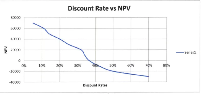
The internal rate of return (IRR) is defined as the discount rate which sets the net present value of a series of cash flows over the study period to zero. It is used as a profit measure since it has been identified as the "marginal efficiency of capital" or the "rate of return over cost". The IRR gives the return of an investment when the capital is in use as if the investment consists of a single outlay at the beginning and generates a stream of net benefits afterwards. Figure 2-1 below shows the IRR when NPV is at zero (Abdelhalim and Kirkham, 2004).
Discount Rate vs NPV
80000 -60000 10000 20000 0 0 -401X)(0 -401oX -Discount Rates - Series1Figure 2-1 Single IRR
It is important to note however, that the IRR does not take into consideration the reinvestment opportunities related to the timing and intensity of the outlays and returns at the intermediate points over the study period. For cash flows with two or more sign changes of the cash flows in any period, multiple values of IRR may exist. in such cases, the multiple values of IRR are subject to various interpretations. The equation for computing the IRR is given below.
Ht'y - Ct'y
NPVy = I =0
t=O
Where: r = IRR
_-Modified IRR (MIRR)
The MIRR and IRR are similar however the MIRR is theoretically superior in that it overcomes certain weaknesses of the IRR. The MIRR takes into account the reinvestment at the project's cost of capital and avoids the problem of multiple IRRs. However, note that the MIRR is not used as widely as the IRR in practice.
Minimum Acceptable Rate of Return (MARR)
MARR or hurdle rate is the minimum rate of return, a company is willing to accept before proceeding with a project, given its risk and the opportunity cost of forgoing other projects. MARR represents the required or minimum internal rate of return for a project investment. There is no distinctive formula for the MARR. This value is usually given and is compared a certain project's IRR. If the IRR is greater than MARR, then the project is deemed to be acceptable.
Payback Period (PBP)
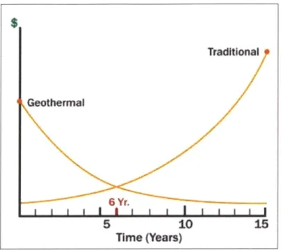
The payback period (PBP) refers to the length of time within which the benefits received from an investment can repay the costs incurred during the time in question while ignoring the remaining time periods in the planning horizon. Even the discounted payback period indicating the "capital recovery period" does not reflect the magnitude or direction of the cash flows in the remaining periods. However, if a project is found to be profitable by other measures, the payback period can be used as a secondary measure of the financing requirements for a project. Take for
example the comparison of having a traditional power plant and a geothermal power plant. This is shown in figure below.
Figure 2-2 Payback Period of Geothermal Plant'
Figure 2-2 shows how the initial investment of a geothermal power plant is much greater than that of a traditional plant. It can also be seen that as time progresses, the costs incurred by the geothermal plant decrease while the traditional plant's costs increase. The time it takes for the two curves to intersect shows the payback period of investing in a geothermal power plant. Figure 2-2 shows that despite having a bigger initial investment in the geothermal plant, the investment starts to pay off after six years into its operation. The equation to calculate the Payback period for any investment is given below.
Payback period = Investment required / Net annual cash inflow
Geothermal
Time (Years)
---Benefit to Cost Ratio
The benefit to cost ratio (BCR) is the ratio of discounted benefits to the discounted costs at the same point in time, is a profitability index based on discounted benefits per unit of discounted costs of a project. It is also known as the savings-to-investment ratio (SIR) when the benefits are derived from the reduction of undesirable effects. Its application also depends on the choice of a study period and an MARR. Since some savings may be interpreted as a negative cost to be deducted from the denominator or as a positive benefit to be added to the numerator of the ratio, the BCR or SIR is not an absolute numerical measure. However, if the ratio of the present value of benefit to the present value of cost exceeds one, the project is profitable irrespective of different interpretations of such benefits or costs.
The benefit-cost ratio is defined as the ratio of the discounted benefits to the discounted cost at the same point in time.
B
BCR=
-(1+r)~BCR=
~(1 +r)'
Where: Bt = Benefits at a certain time; Ct = Cost at a certain time; r = discount rate
While this method is often used in the evaluation of public projects, the results may be misleading if proper care is not exercised in its application to mutually exclusive proposals. However, a project with the maximum benefit-cost ratio among a group of mutually exclusive proposals generally does not necessarily lead to the maximum net benefit. Unfortunately, more
analyses will be required to determine which project has better value. This approach is not recommended for use in selecting the best among mutually exclusive proposals.
Return on Investment (ROI)
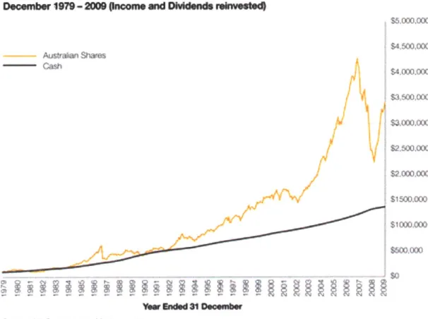
When an accountant reports income in each year of a multi-year project, the series of cash flows must be broken up into annual rates of return for those years. The ROI usually means the accountant's rate of return for each year of the project duration based on the ratio of the income (revenue less depreciation) for each year and the asset value (investment) without depreciation for that same year. Thus, the ROI differs from year to year, with a very low value at the early years and a high value in the later years of the project (Investopedia, 2007). This is typical of construction project since initial costs are incurred by the contractor at the start and payments for services are made at later times of the project duration. Figure 2-3 shows an example of a return on investment of $100,000 from December 1979 - 2009.
Reumw
on ki
nWt
of
$100A00
December 1979 -2009noomj and *W rdeinst
Aujstrar Shafos JAO
S4.000.000
$1500.000
Vaa Enbded310eocamer Source: M4tC %rasmet angement
Austa sarerettns S&ASx 3W0 Accumulaim ide
Figure 2-3 Return on investment3
It can be observed that the ROI at the start is small and increases towards 2007. This is not surprising since most project investments take time to pay off and are not necessarily equal every year.
CHAPTER 3: Life Cycle Cost Models
Depending on the amount of data resources available, time constraints, the degree of accuracy, and other factors such as data availability, four main different ways of performing LCCA exist. These are the Analogy, Parametric, Engineering Cost and Cost Accounting Models. These different methods have their own distinct advantages and disadvantages.
Analogy Models
LCCA's that are produced through an analogy model identify a similar project or component and adjust its costs for differences between it and the target project. It is crude to handle costs this way since direct labor and overhead expenses are not addressed directly. These costs are not accounted for directly, since it simply looks at what the costs have been historically and scales them according to the most important cost driver. Such models can be effectively implemented when extensive historical material is available (Emblemsvag, 2003).
Parametric Models
Parametric Models are considered to be more advanced than analogy models. A parametric
LCCA model involves predicting a project's or a component's cost either in total or for various
activities by using several models describing the relationship between cost and project or process related parameters. These parameters could be:
1. Installation Complexity 2. Design Familiarity
3. Performance
4. Schedule Compression
Compared to the analogy model, three main differences exist. First, the analogy model depends on a single, dominant cost driver whereas a parametric model can use several parameters. Second, an analogy model is based on linear relationships between cost and cost drivers, while parametric models rely on one or more non-linear regression models. Third whereas analogy models use an analogy as a driver, parametric models are regression, or response surface, models that can be linear, quadratic, and multidimensional.
Similar to analogy models, parametric models do not handle overhead costs directly. They also do not go beyond simply presenting an assessment number without any further critical evaluation. These models are limited to some extent but can be useful in certain situations. (Emblemsvag, 2003).
Engineering Cost Models
Engineering Cost Models are employed where there are detailed and accurate capital and operational cost data for the project under study. Unlike the two previous models, it involves direct estimation of a particular cost element by examining the project component by component. Engineering cost models, although offering much more information than analogy and parametric
models are also limited in usage. But as the name suggest, they are very handy in engineering and development situations to obtain an early cost estimate (Emblemsvag, 2003).
Cost Accounting Models
A Cost Accounting Model can be seen as a information system because it relies on definite
information such as units produced and labor hours. Project costs as well as other information can be obtained through a specified costing system methodology. Furthermore, the end results are decided by the costing system which are utilized as same input data and can be used in a variety of ways. Every cost accounting model incorporates a unique approach for utilization of data.
The traditional cost accounting system uses a volume-based, single cost driver. Therefore, the conventional project costing system tends to misrepresent the cost of projects. In a majority of cases, this kind of costing system allocates overhead expenses to the projects based on their comparative utilization of direct labor. It results in the traditional cost systems representing incorrect project costs. The method assumes that a project causes costs and expenditures. Every time the construction of a unit or block of a project takes place, costs are incurred. For a majority of the overhead activities, the share of activity actually used by a particular project does not correspond to a single cost driver. This is true for modem organizations, where products are manufactured through a combination of technology and labor.
The conventional cost accounting model makes use of a volume-based driver such as machine hours or direct labor hours for assigning the total construction overhead expenses. Therefore, a decrease in overhead costs might cause a decrease in quality of projects as compared to a long-lasting reduction in the costs. The quality of the project could decrease if less labor hours and machine hours are spent on it.
Considering the advantages and disadvantages of the different LCCA models, a combination of the Engineering Cost Model and Cost Analysis Model can be selected. Since accurate data on the costs related to the railroad tunnel exists, these two models can be applied to economically evaluate railroad tunnel projects (Emblemsvag, 2003).
CHAPTER 4: Advantages and Disadvantages of Life Cycle Cost
Analysis Evaluation Criteria and Principles of Sensitivity Analysis
Net Present Value (NPV)NPV serves as an indicator of how much value an investment or project adds to the firm. The net
present value of a time series of cash flows, both incoming and outgoing, is defined as the sum of the present values of the individual cash flows.
Advantages:
1. NPV gives the correct decision advice assuming a perfect capital market and will also
rank for mutually exclusive projects.
2. NPV gives an absolute value.
3. NPV considers the time value for the cash flows.
Disadvantages:
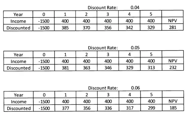
The disadvantage to the use of NPV is its sensitivity and reliance on the discount rates. The discount rate used in the denominators of each present value (PV) computation is critical in determining what the final NPV number will turn out to be. A small increase or decrease in the discount rate will have a considerable effect on the final output. Thus, it is very important and difficult to identify the correct discount rate.
For example, a cash flow with different discount rates but the same cash flow per year is shown in the table 4-1.
Table 4--1 Comparison of Different Discount Rate Effects on the NPV
Discount Rate: 0.04 Year 0 1 2 3 4 5 Income -1500 400 400 400 400 400 NPV Discounted -1500 385 370 356 342 329 281 Discount Rate: 0.05 Year 0 1 2 3 4 5 Income -1500 400 400 400 400 400 NPV Discounted -1500 381 363 346 329 313 232 Discount Rate: 0.06 Year 0 1 2 3 4 5 Income -1500 400 400 400 400 400 NPV Discounted -1500 377 356 336 317 299 185 It can rates.
be observed from the table that the NPV varies significantly with the change in discount
Internal Rate of Return (IRR):
Internal rates of return are commonly used to evaluate the desirability of investments or projects. The higher a project's internal rate of return, the more desirable it is to invest in the project. Assuming all projects require the same amount of up-front investment, the project with the highest IRR would be considered the best and undertaken first.
Advantages:
1. Indicates whether an investment increases or decreases a firm's value
2. Considers all the cash flows of the project
3. Considers the time value of money
4. Considers the risk of future cash flows
Disadvantages:
1. Requires an estimate of the cost of capital in order to make decisions
2. May not give the value maximizing decision when used to compare mutually exclusive projects
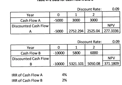
For example, cash flows A and B are to be compared for investment. The data on both cash flows are given by table 4-2.
Table 4--2 Data for Cash Flow A and B
Discount Rate: 0.09
Year 0 1 2
Cash Flow A -5000 3000 3000
Discounted Cash Flow NPV
A -5000 2752.294 2525.04 277.3336
Discount Rate: 0.09
Year 0 1 2
Cash Flow B -10000 5800 6000
Discounted Cash Flow NPV
B -10000 5321.101 5050.08 371.1809
IRR of Cash Flow A
IRR of Cash Flow B
4% 2%
The NPV's for both cash flows were computed. Table 4-2 shows how the IRR does not necessarily produce the value maximizing decision for two mutually exclusive cash flows. It can
be seen that despite cash flow B having a higher NPV than cash flow A, flow B's IRR is less than that of flow A.
3. Cannot be used when the sign of cash flows change more than once during the life of the project
For example, the best way to determine if the IRR can be used is to plot the NPV of the investment against the discount rate of return. This is shown in Figure 4-1 below. To get the IRR, choose the discount rate when NPV intersects the X-axis The IRR for this information can be read of the chart and is determined to be approximately 36.5 percent.
Discount Rate vs NPV
80000 40000 4.f000 0 -20000 -40000 -Series1 Discount RatesFigure 4-1 Single IRR
However, if the NPV crosses the X-axis more than once, i.e. NPV is zero more than once, then the investment is considered to have multiple internal rates of return and should be used with caution. This is shown in the figure 4-2 below.
--Discount Rate vs NPV
35000 30000 25000 20000 15000 C. 10000 5000 0 -S00 -10000 -Seriesi Discount RatesFigure 4-2 Multiple IRR's
Chart 4-2 shows multiple readings for IRR because the NPV intersects the X-axis at four points. It then becomes difficult to choose the correct IRR to represent the project's desirability. It is therefore safer to use IRR when the NPV only touches zero once.
Minimum acceptable rate of return (MARR) or Hurdle Rate:
MARR or hurdle rate is the minimum rate of return on a project a manager or company is willing to accept before starting a project, given its risk and the opportunity cost of forgoing other projects. MARR represents the required or minimum Internal Rate of Return for a project investment.
MARR is compared to the IRR. If the IRR is less than the MARR then the project will not benefit the company.
For example, a firm needs to sell bonds at 8 percent to raise money for a computer. If the IRR of selling bonds is less than the MARR then the company is not benefitting. The MARR should always be higher and not lower than the IRR.
Modified IRR (MIRR):
The MIRR is similar to the IRR, but is theoretically superior in that it eliminates two weaknesses of the IRR. The MIRR correctly assumes reinvestment at the project's cost of capital and avoids the problem of multiple IRR's. However, the MIRR is not used as widely as the IRR in practice.
For example, say a two-year project with an initial outlay of $195 and a cost of capital of 12%, will return $121 in the first year and $131 in the second year. To find the IRR of the project so that the net present value (NPV) = 0:
NPV = 0 = -195 + 121/(1+ IRR) + 131/(1 + IRR)2 NPV = 0 when IRR = 18.66%
To calculate the MIRR of the project, assume that the positive cash flows will be reinvested at the 12% cost of capital. So the future value of the positive cash flows is computed as:
$121(l.12) + $131 = $266.52 = Future Value of positive cash flows at t = 2
Divide the future value of the cash flows by the present value of the initial outlay, which was
$195, and take the square root of the quotient for the 2 periods.
=sqrt($266.52/195) -1 = 16.91% MIRR
It is seen that the 16.91% MIRR is lower than the IRR of 18.66%. In this case, the IRR gives a too optimistic picture of the potential of the project, while the MIRR gives a more realistic evaluation of the project.
Advantages:
1. MIRR correctly assumes reinvestment at project's cost of capital.
2. MIRR avoids the problem of multiple IRR's
Disadvantages:
1. Requires more analysis
Payback Period:
The payback period is the length of time required to recover the cost of an investment.
Advantages:
1. Easy to compute
2. Provides some information on the risk of the investment
3. Gives a crude measure of liquidity
Disadvantages:
1. No concrete decision criteria to indicate whether an investment increases the firm's value
2. Ignores cash flows beyond the payback period
3. Ignores time value of money
Profitability Index or Cost-Benefit Ratio:
Profitability index is a measure that attempts to identify the relationship between the costs and benefits of a proposed project. A ratio of 1 is logically the lowest acceptable measure of the index. A value lower than 1.0 indicates that the project's PV is less than the initial investment. As values on the profitability index increase, so does the financial attractiveness of the proposed project.
Advantages:
1. Shows whether and investment increases the firm's value
2. Considers all cash flows of the project
3. Considers time value of money
4. Considers the risk of future cash flows
5. Useful in ranking and selecting projects when capital is rationed
Disadvantages:
1. Requires an estimate of the cost of capital in order to calculate the profitability index
Accounting rate of return (ARR) or Return on Capital Employed (ROCE) or Return on
investment (ROT):
The ARR method (also called the return on capital employed (ROCE) or the return on investment (ROI) method) of appraising a capital project is used to estimate the accounting rate of return that the project should yield. If it exceeds a target rate of return, the project will be undertaken.
Advantages:
1. It is a particularly useful approach for ranking projects where a firm faces liquidity constraints and requires fast repayment of investments.
2. It is appropriate in situations where risky investments are made in uncertain markets that are subject to fast design and product changes or where future cash flows are particularly difficult to predict.
3. The method is often used in conjunction with the NPV or IRR method and acts as a first screening method to identify projects which are worthy of further investigation.
4. It is easily understood by all levels of management.
5. It provides an important summary method: how quickly will the initial investment break even?
Disadvantages:
2. It implicitly assumes stable cash receipts over time.
3. It is a relative measure rather than an absolute measure and hence takes no account of the size of the investment.
4. It takes no account of the length of the project.
5. It ignores the time value of money.
Summary of Evaluation
As described in the beginning of chapter 1, Life-cycle cost analysis (LCCA) is a method for assessing the total cost of ownership. It is systematic way of considering all costs that could incur from making a certain investment.
Based on the advantages and disadvantages of each economic evaluation criterion mentioned in this chapter, NPV method is selected as a base in evaluating if a project is worth investing in. Among all the criteria, it is the NPV that considers all cash flows, the time value of money, and the risk of future cash flows. Because it takes into account the time value of money and considers the cash flows stream in its entirety, it is in accordance with the financial objective of maximization of the investors' wealth. Thus, in determining the feasibility and attractiveness of investments, it is helpful to see the total cost of a project in the present time value of money.
However, when projecting future costs to the present, there is always a discount rate being applied. This discount rate is very difficult to estimate and influences the NPV greatly since it is taken into account in the NPV's calculation. Thus identifying a correct discount rate is key in coming up with accurate and acceptable results. In essence, the net present value of a project will
help investors see if a project will add to the value of their firm. However, NPV by itself will not be sufficient and will not equip investors with enough information to make sound financial judgments on investments.
In capital investment decision making, there are several ways to evaluate the value of a certain investment. Each of these methods has its own distinct advantages and disadvantages. All other things being equal, using internal rate of return (IRR) and net present value (NPV) measurements to evaluate projects often results in the same findings. However, there are a certain situations where IRR cannot be effectively applied. IRR's major limitation is also its greatest strength: it uses one single discount rate to evaluate every investment.
Although using one discount rate simplifies matters, there are a number of situations that cause problems for IRR. If an analyst is evaluating two projects, both of which share a common discount rate, predictable cash flows, equal risk, and a short time horizon, IRR will probably work. However, a problem exists in that discount rates usually change substantially over time. For example, consider the rate of return on a T-bill in the last 20 years as a discount rate. One-year T-bills returned between 1% and 12% in the last 20 One-years, so clearly the discount rate does change from time to time.
Without modification, IRR does not account for changing discount rates, so it's just not sufficient for longer-term projects with discount rates that are expected to vary. Another type of project for which a basic IRR calculation is ineffective is a project with a mixture of multiple positive and negative cash flows. This was shown early in chapter 4 when multiple values of IRR were produced from the multiple sign changes of NPV.
Another problematic situation for those who use the IRR method is when the actual discount rate of a project is unknown. In order for the IRR to be considered aa a valid evaluator of a project, it must be compared to an actual discount rate. If the IRR is greater than the discount rate, the project should be undertaken otherwise it should not. If a discount rate is not known, or cannot be applied to a specific project for whatever reason, the IRR is of limited value. In these kinds of situations, being able to calculate a positive or negative NPV shows whether a project is feasible or not.
Even if this is the case, IRR is still being used by many. The reason for this may lie in the simplicity of its calculation.
,n RPy Et,y - Ct,y = _ (1+r)" C=O Where:r = IRR
In summary, the NPV method is inherently complex and requires assumptions at each stage such as a discount rate and likelihood of receiving income and others of this sort. The IRR method simplifies projects to a single value that decision makers can use to determine whether or not a project is economically viable (Investopedia, 2007).
Coupling NPV with other evaluation criteria such as IRR and Payback period is ideal since one alone is not sufficient and does not give a clear picture of project costs. All the criteria mentioned can contribute to investment making decisions. Depending on the data available, one can select
criteria that are applicable to certain projects. The application of the NPV method for purposes of this thesis will be discussed in chapter 6.
Principles of Sensitivity Analysis
Decisions having to be made about structure-related investments typically involve a great deal of uncertainty about their costs and potential savings. Performing an LCCA increases the likelihood of choosing a project that saves money in the long run. Yet, there may still be some uncertainty associated with the LCC results. LCCA's are usually performed early in the design process when only estimates of costs and savings are available, rather than certain monetary amounts. Uncertainty in input values means that actual outcomes may differ from estimated outcomes.
There are methods for comparing the cost of different project alternatives. Deterministic techniques, such as sensitivity analysis an breakeven analysis, are done without requiring additional resources or information. These methods illustrate how uncertain input data affect the
analysis outcome.
On the other hand, probabilistic techniques can predict risk and the probability of having different values of economic worth from probability distributions for input values that are uncertain. However, these methods require more information and data than deterministic methods.
For the purposes of thesis however, probabilistic techniques will not be used and are not included in the Life-Cycle Cost Model. This is due to the fact that, so far, the information on input uncertainties is limited.
The Use of Sensitivity Analysis
Sensitivity analysis is effective for:
1. Identifying which uncertain input cost has the greatest impact on a specific measure of
economic evaluation.
2. Determining how variability in the input value affects the range of a measure of economic evaluation.
3. Testing different scenarios.
To determine the critical input parameters, obtain estimates for upper and lower ranges, or change the value of each input parameter up or down, holding all others constant, and recalculate the economic measure to be tested. This is can be seen more clearly in the following section
called Procedure for Sensitivity Analysis.
There are several ways or scenarios in which a sensitivity analysis can be applied to a project. For the purposes of this thesis however, a sensitivity analysis was done to see which input parameter cost would have the greatest impact on the NPV. Also, another sensitivity analysis was conducted to see how different discount rates affect the value of the NPV. The procedure and results for conducting sensitivity analyses is discussed in chapter 6.
CHAPTER
5:
Application of the NPV and Sensitivity Analysis to
the Lotschberg Basis Tunnel
To be able to demonstrate the use of the NPV method and sensitivity analysis, information on annual costs incurred during the first three years (2008 - 2010) of the Ldtschberg Basis Tunnel project was used. Note however that only information on costs and none on benefits is available. Another factor to keep in mind is that there is no actual information on the discount rate for this project. Even if this is the case however, the NPV can still be computed by using different values of the discount rate with the cost data available. Very importantly, the calculated NPV's are very useful for comparing different investment alternatives.
In addition to the application of the NPV method, sensitivity analyses were also conducted to answer two questions:
1. Which annual cost item has the most effect on its corresponding annual PV?
2. What is the effect of varying the discount rate on the NPV?
It is important to note that these are not the only ways of conducting a sensitivity analysis. As mentioned in chapter 4, different questions and scenarios can also be tested. This depends on what the investors or project managers want to achieve in the analysis.
In essence, this chapter will discuss the application and results of applying the NPV method and sensitivity analyses to the Ldtschberg Basis Tunnel project.
Available Information
The L6tschberg Basis Tunnel was completed and started to commercially operate in 2007. The following are major cost components that need to be considered.
1. Construction costs
2. Tunnel maintenance and operations costs
3. Train energy cost
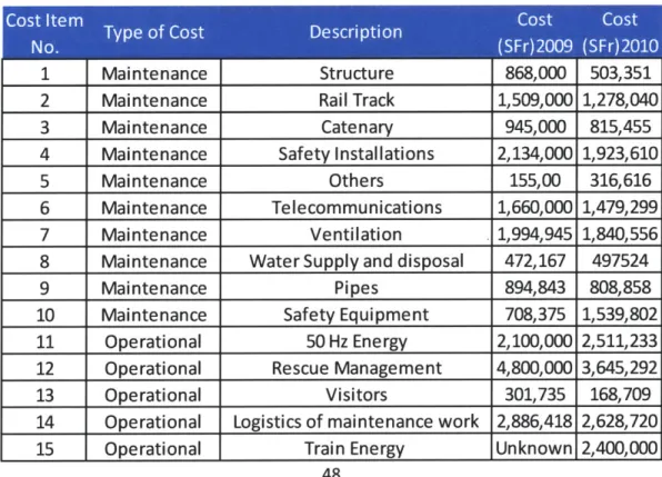
Table 6-1 shows the information on maintenance, operation and train energy costs incurred in the L6tschberg Basis Tunnel project through 2009 and 2010 as provided by the operator. It can be seen that the costs consist mostly of operational and maintenance costs. Each type of cost was assigned a cost item number for easier referencing.
Table 5-1 Summary of Costs
1 Maintenance Structure 868,000 503,351
2 Maintenance Rail Track 1,509,000 1,278,040 3 Maintenance Catenary 945,000 815,455
4 Maintenance Safety Installations 2,134,000 1,923,610
5 Maintenance Others 155,00 316,616 6 Maintenance Telecommunications 1,660,000 1,479,299 7 Maintenance Ventilation 1,994,945 1,840,556
8 Maintenance Water Supply and disposal 472,167 497524
9 Maintenance Pipes 894,843 808,858 10 Maintenance Safety Equipment 708,375 1,539,802 11 Operational 50 Hz Energy 2,100,000 2,511,233 12 Operational Rescue Management 4,800,000 3,645,292
13 Operational Visitors 301,735 168,709
14 Operational Logistics of maintenance work 2,886,418 2,628,720
15 Operational Train Energy Unknown 2,400,000
Application of NPV Method on the Costs of the Ldtschberg Basis Tunnel
As mentioned at the beginning of this chapter, information on the annual costs for the L6tschberg Basis Tunnel is available. These cots are subdivided into three main groups: Operational, Maintenance and Construction costs. Based on these data, an LCCA can now be applied to evaluate its financial worth.
To obtain the NPV of the project, the different costs incurred in the first three years of operation of the railroad tunnel were all converted to their corresponding present values in the base year
(2008). The assumed base year for this project is 2008. In summary, costs in 2008 were assumed
to be construction costs only and operational and maintenance costs came later on in the years
2009 and 2010. Thus, the only costs really influenced by the discount rate are the costs related to
operations and maintenance. Since construction costs occurred during the base year, the denominator in the PV calculation becomes 1 thus leaving the construction cost value as is. Costs from 2009 and 2010 were both projected back to 2008 at discounts rates ranging from 1 to
5 percent. This was done since the value of the actual discount rate was not available. Calculations of the NPV using different discount rates can be seen in Appendix A.
The results of all the calculations yield a negative value. This is acceptable due to the fact that no income data were used in the calculations. Although a complete LCCA would have costs and benefits in its calculation, the results of using only costs is very useful to investors in making a decision, e.g. to compare projects with different alignments.
Table 6-2 below is a summary table; more details when varying the input will be shown later in this chapter.
Table 5-2 Computed NPV's using different discount rates 1% 4,365,000,000.00 21,217,309.90 21,916,473.88 4,408,133,783.78 2% 4,365,000,000.00 21,009,297.06 21,488,845.64 4,407,498,142.70 3% 4,365,000,000.00 20,805,323.30 21,073,612.03 4,406,878,935.33 4% 4,365,000,000.00 20,605,272.12 20,670,298.63 4,406,275,570.75 5% 4,365,000,000.00 20,409,031.43 20,278,453.51 4,405,687,484.94
Application of Sensitivity Analyses to Relevant Data from the Lotschberg Basis Tunnel
As mentioned at the start of the chapter, the goal of applying this sensitivity analyses in this case is to determine which costs are most likely to affect the NPV the most and how a variation of discount rates affects the NPV.
The first question can be answered by varying some selected input cost items. Since there are only a few input costs to vary, a sensitivity analysis was done on each input cost while holding others constant.
As for the second question, the effect of varying the discount rate can be seen by calculating the
NPV using different rates.
Before answering these two questions however, the procedure for sensitivity analysis will first be discussed.
For example, a sensitivity analysis was conducted on the costs given in the table 5-1 using Microsoft Excel's what if function. There are several resources that discuss the procedure of conducting a sensitivity analysis using Microsoft Excel Spreadsheets. The cost of each maintenance and operational item was varied by 10 percent increments. An example for cost item 1 is shown in table 5-3 below.
I
Table 5-3 Impact of Structural Costs to Total Maintenance Costs 607,600.00 11,080,930.00 694,400.00 11,167,730.00 781,200.00 11,254,530.00 954,800.00 11,428,130.00 1,041,600.00 11,514,930.00 1,128,400.00 11,601,730.00
The maintenance cost for the structure for the year 2009 was originally 868,000.00 Swiss francs. The first column of table shows the original value (cell highlighted with red) of the cost as well as its different variations. These different variations are computed by 10 percent increments. For example, 90 and 110 percent of 868,000.00 is 781,200.00 and 954,800.00 respectively. Varying the structural maintenance cost subsequently yielded different values for the total maintenance cost of 2009. The change in values of the total maintenance costs were then correlated to the Present Value of the same year. Table 5-4 shows how much the PV changes with respect to total maintenance cost.
- -- - -
---Structural Maintenance Corresponding Total Costs (varied by 10 percent Maintenance Cost
Table 5-4 Impact of Total Maintenance Cost on the PV of 2009 11,080,930.00 20,161,032.00 11,167,730.00 20,243,699.00 11,254,530.00 20,326,365.00 11,428,130.00 20,491,699.00 11,514,930.00 20,574,365.00 11,601,730.00 20,657,032.00
Since the structural maintenance costs affect the total maintenance cost and in turn also affect the PV of that year, the sensitivity of the PV of 2009 can be determined. Figure 5-1 below shows the effect of having varying total maintenance cost as a result of a varying structural maintenance cost on the PV of 2009. Also, to show the difference in impact of each cost item, the PV as a result of varying cost item 2 is also shown in the figure.
--Impact on PV due to Variation in Cost Items 1 and
2
Corresponding PV's *Original PV of 2009
Millions U Pv due to 70% of item 1
19.80 20.00 20.20 20.40 20.60 20.80 21.00 A PV due to 80% of item 1 1
J
X PV due to 90% of item 1 EX
PV due to 110 % of item 1 *PV due to 120% of item 1 U + PV due to 130% of item 1 2 - -Original PV of 2009Figure 5-1 Cost Items 1 (structure) and 2 (rail track) Impacts on PV of 2009
It can be observed that cost item 2 impacts the PV of 2009 more than cost item 1. This can be
determined by looking at the minimum and maximum values of PV for each of the cost items. The lower and upper boundary for cost item 2 covers a wider range than those of cost item 1.This procedure is repeated for each cost item for 2009 and 2010. All sensitivity analysis tables can be found in Appendix B.
Sensitivity Analysis to Address Question 1
After applying a sensitivity analysis on each of the cost items for 2009 and 2010 separately, question 1 mentioned earlier can now be addressed using the following results. It should be noted that both years had information for cost items 1 through 14 but only 2010 had data for cost item
15 (train energy cost). As for the 2009 results, these can be see be seen in table 5 and figure
5-2 below.
.
Table 5-5 Sensitivity Analysis Results for 2009 1 Structure: 868,000 20,409,032 20,161,032.00 20657,03200 2 Rail Track: 1,509,000 20,409,032 19,977,889.00 20,840,175.00 3 Catenary: 945,000 20,409,032 20,139,032.00 20,679,032.00 4 Safety installations: 2,134,000 20,409,032 19,799,318.00 21,018,746.00 5 Telecommunications: 1,660,000 20,409,032 19,934,746.00 20,883,31&00 6 Ventilation: 1,994,945 20,409,032 19,839,048.00 20979,1&00
7 Water Supply and Disposal: 472,167 20,409,032 20,274,127.00 20,543,937.00
8 Controls 894,843 20,409,032 20,153,362.00 20,664,701.00 9 Safety Equipment: 708,375 20,409,032 20,206,639.00 20,611,425.00 10 Miscellaneous: 155,00 20,409,032 20,364,746.00 2Q453,31&00 11 50 Hz Energy 2,100,000 20,409,032 19,809,032.00 21009,032.00 12 Rescue Management 4,800,000 20,409,032 19,037,603.00 21,780,460.00 13 Visitors 301,735 20,409,032 20,322,822.00 20495,242.00
14 Logistics of Maintenance Work 2,886,418 20,409,032 19,584,341.00 2L233,723.00
15 Train Energy No data 20,409,032
-_-These results show that item number 12 had the greatest impact on the PV of 2009 while item 10 had the least. These two observations can be seen easily in the figure 5-2 as expressed by the difference between a cost item's upper (130 %) and lower (70%) limit PV.