SW2D-LEMON: a new software for upscaled shallow water modeling

HAL Id: hal-03224050

https://hal.inria.fr/hal-03224050

Submitted on 11 May 2021

HAL is a multi-disciplinary open access archive for the deposit and dissemination of sci-entific research documents, whether they are pub-lished or not. The documents may come from teaching and research institutions in France or abroad, or from public or private research centers.

L’archive ouverte pluridisciplinaire HAL, est destinée au dépôt et à la diffusion de documents scientifiques de niveau recherche, publiés ou non, émanant des établissements d’enseignement et de recherche français ou étrangers, des laboratoires publics ou privés.

Joao Guilherme Caldas Steinstraesser, Carole Delenne, Pascal Finaud-Guyot,

Vincent Guinot, Joseph Kahn Casapia, Antoine Rousseau

To cite this version:

Joao Guilherme Caldas Steinstraesser, Carole Delenne, Pascal Finaud-Guyot, Vincent Guinot, Joseph Kahn Casapia, et al.. SW2D-LEMON: a new software for upscaled shallow water modeling. Simhy-dro 2021 - 6th International Conference Models for complex and global water issues - Practices and expectations, Jun 2021, Sophia Antipolis, France. �hal-03224050�

Rousseau – SW2D-LEMON: a new software for upscaled shallow water modeling

SW2D-LEMON:

A

NEW

SOFTWARE

FOR

UPSCALED

SHALLOW

WATER

MODELING

Joao Guilherme Caldas Steinstraesser

Inria, IMAG, Univ Montpellier, CNRS, Montpellier, France joao-guilherme.caldas-steinstraesser@inria.fr

Carole Delenne

Univ Montpellier, HSM, CNRS, IRD, Inria, Montpellier, France

carole.delenne@inria.fr

Pascal Finaud-Guyot

Univ Montpellier, HSM, CNRS, IRD, Inria, Montpellier, France

pascal.finaud-guyot@inria.fr

Vincent Guinot

Univ Montpellier, HSM, CNRS, IRD, Inria, Montpellier, France

vincent.guinot@inria.fr

Joseph Luis Kahn Casapia

Inria, IMAG, Univ Montpellier, CNRS, Montpellier, France

joseph-luis.kahn-casapia@inria.fr

Antoine Rousseau

Inria, IMAG, Univ Montpellier, CNRS, Montpellier, France

antoine.rousseau@inria.fr

KEY

WORDS

Shallow water equations, urban floods, software, upscaling, finite volumes

ABSTRACT

We present a new multi-OS platform named SW2D-LEMON (SW2D for Shallow Water 2D) developed by the LEMON research team in Montpellier. SW2D-LEMON is a multi-model software focusing on shallow water-based models. It includes an unprecedented collection of upscaled (porosity) models used for shallow water equations and transport-reaction processes. Porosity models are obtained by averaging the two-dimensional shallow water equations over large areas containing both a water and a solid phase. The size of a computational cell can be increased by a factor 10 to 50 compared to a 2D shallow water model, with CPU times reduced by 2 to 3 orders of magnitude. Applications include urban flood simulations as well as flows over complex topography. Besides the standard shallow water equations (the default model), several porosity models are included in the platform: (i) Single Porosity, (ii) Dual Integral Porosity, and others are currently under development such as (iii) Depth-dependent Porosity model. Various flow processes (friction, head losses, wind, momentum diffusion, precipitation/infiltration) can be included in a modular way by activating specific execution flags. We recall here the governing equations as well as numerical aspects and present the software features. Several examples are presented to illustrate the potential of SW2D.

1.

In this paper, we present a new multi-OS platform named SW2D-LEMON (SW2D for Shallow Water 2D) developed by the LEMON research team in Montpellier.

Simulating urban floods and free surface flows in wetlands requires considerable computational power. Two-dimensional shallow water models are needed. Capturing the relevant hydraulic detail often requires

computational cell sizes smaller than one meter. For instance, meshing a complete urban area with a sufficient accuracy would require 106 _{to 10}8 _{cells, and simulating one second often requires several CPU seconds. This}

makes the use of such model for crisis management impossible. Similar issues arise when modelling wetlands and coastal lagoons, where large areas are often connected by an overwhelming number of narrow channels, obstructed by vegetation and a strongly variable bathymetry. Describing such channels with the level of detail required in a 2D model is impracticable. A new generation of models overcoming this issue has emerged over the last 20 years: porosity-based shallow water models. They are obtained by averaging the two-dimensional shallow water equations over large areas containing both water and a solid phase [8]. The size of a computational cell can be increased by a factor 10 to 50 compared to a 2D shallow water model, with CPU times reduced by 2 to 3 orders of magnitude. Research on porosity-based shallow water models has accelerated over the past 15 years, with significant contributions led by V. Guinot and our research team [1], [2], [3], [4], [13], [15], [20].

SW2D-LEMON is the software continuation of this 15 years research production. It follows the original research code first developed by V. Guinot in Fortran 90. SW2D-LEMON is multi-platform (Linux, MacOS, Windows) and includes a convenient graphical user interface (GUI) together with an unprecedented collection of upscaled (porosity) models used for shallow water equations and transport-reaction processes. Applications include urban flood simulations as well as flows over complex topography with unstructured grids. Besides the standard shallow water equations (the default model), several porosity models are already included in the platform such as Single Porosity and Dual Integral Porosity. Various flow processes (friction, head losses, wind, momentum diffusion, precipitation/infiltration) can be included in a modular way by activating specific execution flags.

The paper is organized as follows: in Section 2, we recall the traditional shallow water equations as obtained by Saint-Venant, before defining the notion of porosity, presenting the single and dual porosity models and then the (standard) features of the numerical schemes used in the code. Section 3 describes the SW2D-Lemon workflow by presenting the inputs and outputs as well as the different options available to the modeler. Section 4 presents the three different licenses provided for the software before illustrating the installation process under Windows. Finally, we end this article with a presentation of the test cases that are provided in version 1.0 of the code, that will be made available to the Polytech'Montpellier engineering school from September 2021. For the sake of simplicity, the SW2D acronym will hold for SW2D-Lemon hereafter. For more information on SW2D-LEMON, please visit http://sw2d.inria.fr

2. M

2.1 Equations and source terms

The current version of the SW2D simulation engine incorporates the Shallow Water Equations (SWEs), the Single Porosity (SP) [1] and the Dual Integral Porosity (DIP) [2] models. Other models published by members of the LEMON team, such as the Multiple Porosity (MP) [3] and Depth-Dependent Porosity (DDP) [4] models, are currently under integration and testing and should be released soon. The governing equations for these three models can be written in the form

𝜕"𝐮 + 𝐌 ∇. 𝐅 = 𝐬 (1)

where t is time, u and s are respectively the conserved variable and source term vectors, and F and M are respectively the flux and inertia tensors.

The SWE model, an extension of Saint Venant’s one-dimensional equations [5], uses the following definitions for u, s, F and M: 𝐮 = ,ℎ𝑢ℎ ℎ𝑣0 , 𝐬 = 2 𝑅 − 𝐼 𝑔ℎ7𝑆9,:− 𝑆;,:< − 𝐼𝑢 + 𝑊: 𝑔ℎ7𝑆9,>− 𝑆;,>< − 𝐼𝑣 + 𝑊> ? (2a) 𝐅 = 2 ℎ𝑢 ℎ𝑣 ℎ𝑢@_{+ 𝑔ℎ}@_{/2 ℎ𝑢𝑣} ℎ𝑢𝑣 ℎ𝑣@_{+ 𝑔ℎ}@_/2? , 𝐌 = 𝐈𝐝 (2b)

Rousseau – SW2D-LEMON: a new software for upscaled shallow water modeling where 𝑔 is the gravitational acceleration, ℎ is the water depth, 𝑢 and 𝑣 are respectively the 𝑥 − and 𝑦 −components of the flow velocity, 𝐼 is the infiltration rate, 𝑅 is the rainfall intensity, 𝑆_9,G and 𝑆_;,G (𝑋 = 𝑥, 𝑦) are respectively the bottom and friction slopes in the 𝑋 − direction, and 𝑊_G(𝑋 = 𝑥, 𝑦) is the wind drag specific force in the 𝑋 − direction. An eigenvalue analysis of this model is provided in [6]. The wind drag force is computed using Smith and Banke’s model [7].

The SP model was first introduced in a depth-dependent version [7] to model the effects of subgrid scale topography. A depth-independent version for the modelling of urban floods was presented in non-conservation form [8] and later adapted for shock-capturing finite volume methods and discontinuous urban feature properties [1]. In this model, u, s, F and M are defined as

𝐮 = 𝜙 ,ℎ𝑢ℎ ℎ𝑣 0 , 𝐬 = 2 𝑅 − 𝜙𝐼 𝜙𝑔ℎ7𝑆9,:− 𝑆;,:< + 𝑔ℎ𝜕:𝜙 − 𝜙𝐼𝑢 + 𝜙𝑊: 𝜙𝑔ℎ7𝑆9,>− 𝑆;,>< + 𝑔ℎ𝜕>𝜙 − 𝜙𝐼𝑣 + 𝜙𝑊> ? (2a) 𝐅 = ϕ 2 ℎ𝑢 ℎ𝑣 ℎ𝑢@_{+ 𝑔ℎ}@_{/2 ℎ𝑢𝑣} ℎ𝑢𝑣 ℎ𝑣@_{+ 𝑔ℎ}@_/2? , 𝐌 = 𝐈𝐝 (2b)

where 𝜙 is the plan view fraction of space available to water. Porosity models are derived from the SWEs (1, 2a-b) by performing a volume averaging [9] over a control volume containing a water and a solid phase. The underlying assumption of the SP model is that the statistics of the water-solid partition converge to the same values when computed over a horizontal 2D domain and over its boundary. As noticed in [10], this is equivalent to assuming the existence of the Reference Elementary Volume (REV) [11], an assumption that does not hold in typical urban areas [3].

The DIP model [2] was introduced as an improved version of the Integral Porosity model [10]. It uses the following definitions for the terms in Equation (1)

𝐮 = 𝜙M, ℎ ℎ𝑢 ℎ𝑣0 , 𝐬 = 2 𝑅 − 𝜙M𝐼 𝜙M𝑔ℎ7𝑆9,:− 𝑆;,:< + 𝑔ℎ𝜕:(𝜙N− 𝜙M) − 𝜙M𝐼𝑢 + 𝜙M𝑊: 𝜙M𝑔ℎ7𝑆9,>− 𝑆;,>< + 𝑔ℎ𝜕>(𝜙N− 𝜙M) − 𝜙M𝐼𝑣 + 𝜙M𝑊> ? (3a) 𝐅 = ⎣ ⎢ ⎢ ⎢ ⎡_R 𝜙Mℎ𝑢 𝜙Mℎ𝑣 S T RUℎ𝑢 @_{+ 𝜙} M𝑔ℎ@/2 RS T RUℎ𝑢𝑣 R_ST R_Uℎ𝑢𝑣 R_ST R_Uℎ𝑣 @_{+ 𝜙} M𝑔ℎ@/2⎦⎥ ⎥ ⎥ ⎤ , 𝐌 = Y1 0_{0 𝐃}] 𝐈𝐝 (3b) 𝐃 = 𝜖𝐑 `𝜇b 0 0 𝜇@c 𝐑 db_{, 𝜖 = e}1 if 𝜕"ℎ > 0 0 if 𝜕"ℎ ≤ 0 (3c)

where 𝜙_N and 𝜙_M are respectively connectivity and storage porosities, 𝜇_j (𝑘 = 1,2) is a momentum dissipation coefficient (between 0 and 1) in the kth principal direction, and R is the rotation matrix that transforms the x-direction into the first principal x-direction of D. The purpose of the dissipation tensor D is to model the momentum dissipation arising from the multiple wave reflections against obstacles on the subgrid scale. This term is active only in the presence of positive waves, hence the 𝜖 switch (𝜖 = 0 or 𝜖 = 1) in Eq. (3c). In contrast with a classical source term in Eq. (1), the inertia-modifying tensor M preserves the self-similar properties of the solution when Riemann problems are dealt with. This self-similarity property was identified in [3], verified in [2], [4] and confirmed in [12] by numerical experiments. So far, no model has been proposed for the dissipation coefficients 𝜇j as functions of the hydraulic conditions and urban geometry, and the momentum dissipation tensor D must be calibrated.

For all three models (1), (2) and (3), arbitrary initial conditions may be provided. The standard (time-dependent) boundary condition types handled by the models are the following:

– prescribed unit discharge (inflowing or outflowing), – prescribed water depth,

– prescribed free surface elevation, – prescribed Froude number.

In all four cases, if the water is flowing into the domain, the flow velocity vector is assumed normal to the boundary. If the water is flowing out of the domain, the lateral component of the momentum is advected with

the flow. An impervious boundary is considered as a particular case of a prescribed unit discharge boundary, with the normal discharge set to zero.

2.2 Numerical aspects

Equation (1) is solved numerically using a finite volume approach on unstructured grids. Explicit, Godunov-type shock-capturing methods are used for the solution of the hyperbolic part. The algorithm is designed so as to allow for elements with an arbitrary number of edges. Therefore, the mesh may be a mixture of triangular, quadrangular or any type of polygonal elements. Besides, the cells are not required to be convex.

The solution procedure involves a first-order time splitting [13]. Within a computational time step, the sequence is the same for all models:

1) Hyperbolic part

1.1) Determine the maximum permissible time step based on CFL requirements for solution stability on arbitrary-shaped grids [14].

1.2) Reconstruct the flow variables in case a higher-order reconstruction is used (MUSCL-EVR scheme [15][14]).

1.3) Compute the fluxes and the source terms induced by porosity gradients and topography gradients across the interfaces (including boundary interfaces) between the computational cells using approximate, HLLC-type [15] [16] Riemann solvers. In order to speed up the computational process, the user is allowed to specify a threshold water depth. When the water in two neighbouring cells is smaller than this threshold, the two cells are assumed dry and zero fluxes are set automatically across the interface. The details of the Riemann solvers used can be found in the references for the SP and DIP models [1] [2].

1.4) Carry out a mass and momentum balance over the non-dry cells.

1.5) Apply the momentum dissipation tensor D to the cells where the water level has been identified as rising as a result of Step 1.4.

1.6) Revise the balance using a divergence correction procedure in case negative water depths are obtained. Two options are available when the water depth becomes negative within a given cell : (i) all the fluxes across the interfaces of the cell under concern are multiplied by the same factor so as to obtain a zero water depth, or (ii) the computational time step is decreased to the maximum possible value that yields a zero water depth.

2) Compute the effect of source terms. All source terms are local functions of the average flow variables within a given computational cell, which involves solving only local, first-order ordinary differential equations with respect to time within each cell. The contributions of the various source terms are computed sequentially

2.1) Compute the effects of friction. The user can specify the friction model formulation (Manning, Strickler, Chezy, etc.)

2.2) Compute the effects of precipitation/infiltration 2.3) Compute the effects of wind shear stress

It is worth noting that the MUSCL-EVR approach [14] used in the hyperbolic part is significantly computationally cheaper than the classical second-order time stepping MUSCL approach (also called MUSCL-Hancock [18]), because it involves a single step time integration and the reconstruction of a single variable (the free surface elevation) instead of three in the usual procedure.

3. S

SW2D is multi-platform and runs on Linux, MacOS and Windows. It includes all models presented in Section 2 above: classical Shallow Water models, SP and DIP porosity models (other porosity models are currently being implemented and will be available in next software releases). It can be used with any initial data and with the four boundary condition types mentioned above. Several types of forcing (precipitation, infiltration, wind, friction) are also implemented.

Rousseau – SW2D-LEMON: a new software for upscaled shallow water modeling 3.1 Input files

SW2D requires input files providing geometry information, initial and boundary conditions, forcing terms, parameter values, etc. Here we briefly describe the files needed for a simulation (for more details, see the online documentation on the SW2D site):

- Mesh file: SW2D is compatible with the 2DM format (ascii files) provided by the Surface-water Modeling System (SMS) Aquaveo(c) software. SMS can be downloaded from the Aquaveo website. Alternatively, users may generate 2DM file from their own data using Python modules such as Py2DM. It is also possible to convert 2D Selafin/Seraphin files (TELEMAC-MASCARET format) using a dedicated executable included in the SW2D distribution.

The mesh is unstructured. The computational cells may have an arbitrary number of edges. It is for example possible to mix triangles with quadrangles, as long as these meshes are correctly defined in the 2DM file. The 2DM format incorporates the elevation of the mesh nodes, so that no additional elevation data file is needed.

Input files are processed by the sw2dConverter program. This converter produces a binary file containing all the necessary information for the main SW2D program. The format of this binary file is specific to SW2D. As stressed above, sw2dConverter can read files of various formats, such as those from SMS, BlueKenue or Telemac-Mascaret.

- Initial condition file: this text file specifies the initial state of the simulation. The well-posedness of the shallow water problem requires that the initial water level/depth and the components of the flow velocity/unit discharge vector be specified for all computational cells. Two options are made available to the user. If the initial state is uniform, only one line is needed (Figure 1). The values read within this line are applied uniformly to all cells. Otherwise, the initial values are specified on a cell-by-cell basis, with one line containing the 3 initial state variables for each cell in the mesh.

Figure 1: Content of an IC file for water at rest (surface elevation = 1m)

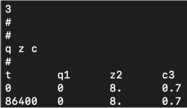
- Boundary condition time series file: this file provides the time series for all the boundary conditions used in the simulation. The time series are placed after a header specifying the number n and the types of boundary conditions. They are arranged in the form of n + 1 columns. For each line, the first column is the time value (in seconds) and the remaining n + 1 records indicate the numerical value of the boundary condition at this specific time (Figure 2). During the simulation, the numerical value of the boundary condition is interpolated using the nearest two times in the file. When the simulated time is larger than the largest time in the time series file, the last read boundary condition numerical value is used.

Figure 2: Content of a BC file with 3 types of boundary conditions, all constant in time: zero discharge, free surface at 8m and Froude number equals to 0.7.

Changes in the last line would lead to time interpolation for q (resp. z,c) at boundary 1 (resp. 2, 3) between t=0 and t=86400

- Input SW2D file: this file specifies the simulation settings: choice of the physical model (shallow water, SP, DIP, etc.), physical and numerical settings (simulation time time, type of boundary

conditions, CFL constraint, type of finite volume scheme) and output parameters (type and frequency of simulation result writing). These parameters are assigned a default value (see the SW2D documentation for more details) that may be overwritten by the user (Figure 3).

Figure 3: Sample SW2D input file. The dual integral porosity (DIP) model is solved using the first-order Godunov scheme. The simulated time is 100 s, the maximum permissible computational time step (dtmax) is 1 second and the simulation results are stored

in the form of maps every second.

- [Optional]: depending on the physical models (porosity, friction, source terms, etc), additional files are needed for the specification of the corresponding model parameters. The format for such files is provided in the software documentation, along with sample files.

3.2. Output files

The model outputs are stored every dtmap seconds. A unique (ascii) output file is created for each stored time. The simulation results are stored on a cell-by-cell basis, with one line for each cell (Figure 4). The verbosity of the storage is controlled in the SW2D input file by a flag that may take 3 values:

- ‘none’: nothing is stored

- ‘standard’: main variables are stored (x, y, zb, h, q, r)

- ‘all’: all variables are stored (main variables above, plus with additional ones such as velocities, free surface elevation, Froude number, etc.)

Figure 4: Sample output file (verbosity flag set to ‘standard’).

3.3 SW2D workflow

The simulation workflow (Figure 5) consists of two main steps. The first step is geometry preprocessing. It consists in converting the mesh and boundary condition input files to the specific format required by the computational engine. The second step is the hydrodynamic computation itself. These two steps are distinct because the geometry processing step can be time-consuming and needs to be done only once. This allows the same model mesh and geometry to be used in numerous simulation scenarios without having to process the mesh again.

SW2D is provided with a Graphical User Interface (GUI) that makes it possible to launch and visualize the simulation progress without the need for external tools (see Section 5). Experienced users may also choose to bypass the GUI and use the software in command line mode. In both cases, the output files are stored in a

Rousseau – SW2D-LEMON: a new software for upscaled shallow water modeling dedicated directory, at a frequency chosen by the user thanks to the dtmap parameter. During the program execution, a number of log messages can be displayed by the user in a dedicated window (or in the console): information, warnings and errors.

Figure 5: Workflow for SW2D execution

4. L

4.1 Licensing

SW2D is the property of Inria (Institut National de Recherche en Informatique et Automatique) and UM (Université de Montpellier). It has been developed in C++ by researchers of the LEMON project-team (common to Inria, UM, CNRS and IRD). Although it is still under development, it is already distributed under 3 different types of licences:

Public Research License

Inria and UM grant to the academic user, a free of charge, without right to sublicense, nonexclusive right to use the software for research purposes for a period of one year.

Private Licence

Inria and UM provide SW2D to any private user (including companies) within the framework of a contract between the parties.

Educational Licence

Inria and UM have formed partnerships with engineering schools where SW2D is distributed free of charge, strictly within the framework of the training of engineering students.

If results obtained through the use of SW2D were to be published, authors should cite corresponding articles, taking information from the SW2D publication page. The software is provided only as a compiled library file. Any decompiling process is strictly unauthorized. Upon request (in the framework of research partnerships), any partner may become a member of the SW2D development team and be granted access to the SW2D C++ source code.

4.2 Installing SW2D

This section presents the example of a binary installation file for Windows, similar to the one provided to educational partners. The process is similar to any Windows program installation (see Figure 6 and Figure 7).

1. Request the sw2d-install-windows.exe file from the SW2D consortium and download it. 2. Locate and double-click the downloaded .exe file. It will usually be in the ‘Downloads’ folder. 3. A dialog box will appear. Follow the instructions to install the software.

4. The software will be installed. For more convenience, it is recommended to add shortcut icons on the user desktop.

Figure 6: Installation process under windows: first steps

Figure 7: Installation process under windows: last steps

Sample files, which allow testing the software, are provided with the installation along with a user's guide.

5.

The present section focuses on different test cases built for teaching. They exhibit the different features of SW2D as the principal points where the 2D flow modeler should pay attention to.

5.1 Gardon test case

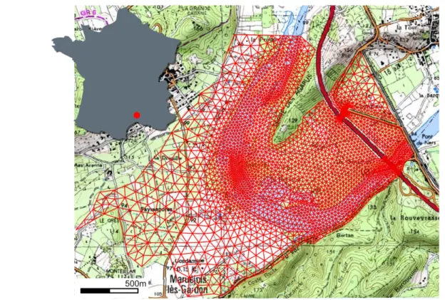
This test case aims to model a flood propagation in the Gardon river near Ners (downstream of Alès, France). It is part of the teaching curriculum at Polytech Montpellier. This site corresponds to the typical configuration where a 2D model should be used, with a sharp meander and a complex channel geometry inducing drying beds, flow divertion into parallel branches and highly non-uniform velocities across the channel section. The channel is also subjected to widening and narrowing, inducing significant transverse flow velocities. Hydraulic structures are also present: a strong narrowing of the floodplain near the downstream section due to a road embankment and a sill (with a 45 degrees angle with the main flow direction) with elevation variation of nearly 2m potentially leading to transcritical flow on the steep downstream slope. This test case is therefore rather synthetic of typical river hydraulics complexities, with mixed and competing influences of geometry, hydraulic parameters and boundary conditions.

Rousseau – SW2D-LEMON: a new software for upscaled shallow water modeling

Figure 8: Gardon test case situation and mesh (basemap ©IGN http://geoportail.gouv.fr).

The hydraulic model is the classical 2D shallow water model. The simulation input files are specified in Table 1.

Table 1: Input files for the Gardon test case.

File name Object

friction_strickler_map.txt Distribution of the friction coefficient (uniform with 𝐾 = 50𝑚b/q_{. 𝑠}db₎

Gardon.2dm Mesh file (5178 unstructured cells)

Gardon.bc Boundary condition file

hydro_boundary_time_series.txt Boundary condition time series (prescribed hydrograph upstream, time-dependent Froude number downstream)

initial_conditions_map.txt Initial conditions map (uniform water level and zero flow assigned uniformly to all cells)

input.sw2d SW2D input file

The flood propagation is simulated with a prescribed upstream unit discharge rising from 0.1m2_{/s to 15m}2_/s.

Figure 9 shows the results obtained at the peak time of the inflowing hydrograph. As shown in the screen capture, the GUI allows for a split view to visualise several variables at the same time.

Figure 9: Visualization in the SW2D GUI of results obtained for Gardon test case near the beginning of the flood pic. Left: surface elevation (the ground elevation is displayed when there is no water in the cell). Right: water depth.

5.2 Sacramento test case

The purpose of this second test case is to illustrate the use of different shallow water models in SW2D, namely the classical shallow water model (SW) and the DIP model described in Section 2. It also aims to illustrate the application of upscaled and fast models to hazard modeling.

This test case, introduced in [2], consists in an hypothetical flood scenario in a neighbourhood of West Sacramento (CA, USA), whose average ground elevation (4m) is below the water elevation (8m) in the Sacramento River Deep Water Ship Channel, which runs parallel to the neighbourhood in the North-South direction. An instantaneous failure is supposed to take place in the levee protecting the urban zone, forming a 100 m wide breach with bottom elevation 5 m.

The fine (SW) and the coarse (DIP) models are solved in unstructured meshes with respectively 78840 and 2529 cells, with average areas within the neighbourhood of 3.6m2 _{and 345m}2 _{respectively. The cell storage}

Rousseau – SW2D-LEMON: a new software for upscaled shallow water modeling

Figure 10: Cell porosity field for the DIP simulation of the Sacramento test case.

The initial conditions for the simulations are a zero velocity and free surface elevations of 8 m in the Water Channel and 4 m within the neighbourhood respectively. Regarding the boundary conditions, a free surface elevation of 8 m is prescribed upstream and downstream the water channel to maintain a constant elevation; impermeable boundaries are set in the undamaged levee and along the Western bank of the Channel; a prescribed Froude number of 0.9 is prescribed along the boundary of the neigbourhood to prevent artificial wave reflection).

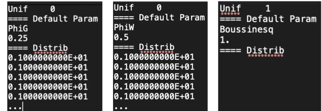
The input files for the SW and DIP simulation are listed respectively in Table 2 and Table 3. Note that the latter requires three extra files, containing distribution of the cell and edge porosities and the Boussinesq coefficient (set uniform and equal to 1). These additional files are presented (partially) in Figure 12. Moreover, as shown in Figure 11; modifications in the input file input.sw2d are minimal.

Table 2: provided files for the classical SW simulation of the Sacramento test case.

File name Object

ModSW.2dm Mesh file (78840 unstructured cells)

ModSW.bc Boundary condition file

hydro_boundary_time_series.txt Timeseries at the boundaries initial_conditions_map.txt Distribution of the initial conditions

Table 3: Provided files for the DIP simulation of the Sacramento test case

File name Object

ModDIP.2dm Mesh file (2529 unstructured cells)

ModDIP.bc Boundary condition file

hydro_boundary_time_series.txt Timeseries at the boundaries initial_conditions_map.txt Distribution of the initial conditions DIP_cell_porosity_map.txt Distribution of the cell porosity parameter DIP_edge_porosity_map.txt Distribution of the edge porosity parameter Boussineq_map.txt Distribution of the Boussinesq coefficient

input.sw2d SW2D input file

Figure 11: input.sw2d files for the swes (left) and DIP (right) simulations of the Sacramento test case.

Figure 12: DIP_cell_porosity_map.txt (left), DIP_edge_porosity_map.txt (middle) and Boussineq_map.txt (right) files for the DIP simulation of the Sacramento test case. The two first files are partially presented, since they contain values for all cells and edges, respectively (Unif is set to 0, so the default value is ignored). The third file is fully presented.

Rousseau – SW2D-LEMON: a new software for upscaled shallow water modeling

Figure 13: water depth (top row) and unit discharge norm (bottom row) at t = 120s for the SW (left column) and DIP (right column) simulations of the Sacramento test case. The color bars were adjusted for a better visualization of the solution within the neighbourhood. The water depth in the Water Channel is constant and equal to 8 m.

6. C

SW2D-LEMON is a new software platform dedicated to shallow water modelling. While the software allows, as many existing software already do, the traditional shallow water equations to be used, its main asset lies in the implementation of various porosity models developed over more than 15 years by our team. Such models, that are upscaled versions of the shallow water equations, allow for a reduction in CPU time up to 3 orders of magnitude. They make real-time simulations over large areas possible.

The present communication marks the release of the first public version of the software (1.0), that is currently used by a few design offices and an engineering school. We have presented the working principles of the code as well as test cases and illustrations of the user interface, allowing for an overview of the broad capabilities of the software.

The SW2D software is under constant evolution. Forthcoming developments include the integration of the Multiple Porosity (MP) [3] and Depth-Dependent Porosity (DDP) [4] models, currently implemented as separate Fortran code versions. The objective is to better answer user needs in terms of numerical models that are at the same time simple, robust and accurate.

While the present communication focuses mainly on the Education version owing to lack of space, the research/development version includes many additional features, such as developer documentations and procedures. These include specific version management procedures, including a testing, validation and documentation writing workflow. It is expected that the SW2D development infrastructure will be viewed by the international community as a platform for the collaborative development of shallow water-based models in the future. New features will be progressively integrated into the software in later versions that can be found at http://sw2d.inria.fr.

REFERENCES

[1] V. Guinot et S. Soares-Frazão, «Flux and source term discretization in two-dimensional shallow water models with porosity on unstructured grids,» International Journal for Numerical Methods in FLuids, vol. 50, pp. 309-345, 2006.

[2] V. Guinot, B. F. Sanders et J. E. Schubert, «Dual integral porosity shallow water model for urban flood modelling.,» Advances in Water Resources, vol. 103, pp. 16-31, 2017.

[3] V. Guinot, «Multiple porosity shallow water models for macroscopic modelling of urban floods,»

Advances in Water Resources, vol. 37, pp. 40-72, 2012.

[4] V. Guinot, C. Delenne, A. Rousseau et O. Boutron, «Flux closures and source term models for for shallow water models with depth-dependent integral porosity,» Advances in Water Resources, vol. 122, pp. 1-26, 2018.

[5] A. J. C. Barré de Saint-Venant, «Théorie du mouvement non permament des eaux, avec application aux crues des rivières et à l'introduction des marées dans leur lit,» Comptes Rendus des Séances de l'Académie

des Sciences, vol. 73, pp. 147-154 and 237-240, 1871.

[6] A. Daubert et O. Graffe, «Quelques aspects des écoulements presque horizontaux à deux dimensions en plan et non permanent, application aux estuaires,» La Houille Blanche, n° %18, pp. 847-860, 1967. [7] S. D. Smith et E. G. Banke, «Variation of the sea surface drag coefficient with wind speed,» Quarterly

Journal of the Royal Meteorological Society, vol. 101, pp. 665-673, 1975.

[8] A. Defina, «Two-dimensional shallow flow equations for partially dry areas,» Water Resourves

Research, vol. 36, pp. 3251-3264, 2000.

[9] J. Hervouët, R. Samie et B. Moreau, chez International Seminar and Workshop on Rescue Actions Based

on Dambreak Flow Analysis, Seinâjoki, Finland, 2000.

[10] S. Whitaker, The method of volume averaging, Springer, 1999.

[11] B. F. Sanders, J. E. Schubert et H. A. Gallegos, «Integral formulation of shallow-water equations with anisotropic porosity for urban flood modeling,» Journal of Hydrology, vol. 362, pp. 19-38, 2008. [12] J. Bear, Dynamics of fluids in porous media, New York: American Elsevier Publishing Company, 1972. [13] V. Guinot, «A critical assessment of flux and source term closures in shallow water models with porosity

for urban flood simulations,» Advances in Water Resources, vol. 109, pp. 133-157, 2017.

[14] G. Strang, «On the construction and comparison of difference schemes,» SIAM Journal on Numerical

Analysis, vol. 5, pp. 506-517, 1968.

[15] S. Soares-Frazão et V. Guinot, « An eigenvector-based linear reconstruction scheme for the shallow water equations on two-dimensional unstructured meshes,» International Journal for Numerical

Methods in Fluids, vol. 53, p. 23–55, 2007.

[16] B. Van Leer, Journal of Computational Physics, vol. 23, pp. 276-299, 1977.

[17] A. Harten, P. D. Lax et B. Van Leer, «On upstream differencing and Godunov-type schemes for hyperbolic conservation laws,» SIAM Review, vol. 25, pp. 35-61, 1987.

[18] E. F. Toro, M. Spruce et W. Speares, «Restoration of the contact surface in the HLL-Riemann solver,»

Shock Waves, vol. 4, pp. 25-34, 1994.

Rousseau – SW2D-LEMON: a new software for upscaled shallow water modeling [20] S. Soares-Frazão et V. Guinot, «An eigenvector-based linear reconstruction scheme for the

shallow-water equations on two-dimensional unstructured meshes,» International Journal for Numerical