Development of an acoustic vorticity meter to measure shear in ocean-boundary layers

DEVELOPMENT OF AN ACOUSTIC VORTICITY METER TO MEASURE SHEAR IN OCEAN-BOUNDARY LAYERS

by

Fredrik Turville Thwaites

B.S., Massachusetts Institute of Technology (1981) S.M., Massachusetts Institute of Technology (1986)

Submitted in partial fulfillment of the requirements for the degree of

Doctor of Philosophy at the

MASSACHUSETTS INSTITUTE OF TECHNOLOGY and the

WOODS HOLE OCEANOGRAPHIC INSTITUTION September 1995

0 Fredrik T. Thwaites, 1995

The author hereby grants to MIT permission to reproduce and to distribute copies of this thesis document in whole or in part.

Signature of Author... ... ... .. .. .... Joint Program in Applied Ocean Science and Engineering

Massachusetts Institute of Technology Woods Hole Oceanographic Institution Certified by... .

/

Senior Scientist, Woo Hole Oceanographic Institution

Thesis Supervisor

Accepted by... ... ... . ... ..

Arthur B.laggeroer

Chairman Joint Committee for Oceanographic Engineering

.,A•U.:,••f SET TS '!N-S' UTE OF TECHNOLOGY

SEP

2 1 1995r

E,•

DEVELOPMENT OF AN ACOUSTIC VORTICITY METER TO MEASURE SHEAR

IN OCEAN-BOUNDARY LAYERS

by

Fredrik Turville Thwaites

Submitted to the Department of Mechanical Engineering and to the Joint Committee for

Applied Ocean Science and Engineering, Massachusetts Institute of Technology and

Woods Hole Oceanographic Institution, September 1995, in partial fulfillment of the

requirements for the degree of Doctor of Philosophy.

ABSTRACT

This thesis describes the analysis and development of an acoustic vorticity meter to measure shear in ocean-boundary layers over smaller measurement volumes than

previously possible. A nonintrusive measurement ofvorticity would filter out irrotational

motion such as surface waves and currents that can swamp small scale measurements of

shear. The thesis describes the desired geophysical measurements and translates this

oceanographic context into design goals.

The instrument was designed, built, tested, and deployed. It measures three-axis

vorticity at 0.83 and 2.45 meters below the ocean surface with measurement volumes of

0.45 meters on a side. The instrument forms a buoy that is inertially instrumented to

calculate and remove buoy motion from the measurements. The instrument uses a

complementary filter algorithm to estimate attitude and motion from low-power,

inexpensive, strapdown rate gyros, accelerometers, and fluxgate magnetometers. The

instrument performance has been measured to have a vorticity bias of not more than 1

10-2 per second in a mean flow of 0.7 meters per second, a bias of not more than 1

10.2

per second in the down-wave and vertical directions in typical ocean waves, and a 30

decibel spectral rejection of surface wave velocity.

Two instrument deployments are described to show the potential of the system.

The instrument has measured shear in the upper-ocean-boundary layer, and these

measurements are compared to concurrently measured wind stress and stratification. The

instrument was also deployed, tethered in the thermocline, in an area of high internal wave

activity. Richardson-number time series were measured and compared favorably to

concurrently measured Richardson numbers made over a larger spatial scale.

Thesis Supervisor: Albert J. Williams III.

Title: Senior Scientist

Acknowledgments

I would like to thank the members of my thesis committee; Eugene Terray, John

Trowbridge, Robert Weller, David Wilson, and Albert Williams III; for their helpful

suggestions for improving the clarity of the text and for serving on my committee.

Particular thanks go to Albert J. (Sandy) Williams III whose experience, good humor, and

generous help greatly assisted me in this work.

The engineers, machinists, welders, and technicians at WHOI are also recognized

for their skills, judgement, and work in helping turn an idea into a practical working

instrument. Particular thanks go to Martin Woodward (Woody), Gary Stanbrough,

Terrence Rioux, Ken Doherty, and Richard Koehler.

Jim Edson and Jeff Hare made the windstress measurements during the Buzzards

Bay Deployment. I thank the Parson's Lab at MIT for the use of a wave tank and laser

doppler velocimeter. I thank the Coastal Research Center for the use of their shop. The

new Bedford Regional Vocational School built a large tank that I used for testing and

calibrating the instrument. I thank Laura Predario for reading the thesis and providing

editing advice. I thank Markku Santala and Todd Morrison for help in the lab.

Support for this project was received from National Science Foundation grants

OCE-9018623 and OCE-9314357, Office of Naval Research grant N00014-89-J-1058,

and a Keck Foundation instrumentation initiative grant.

TABLE OF CONTENTS

Page No.

Abstract ... 3

Acknowledgments ... 4

List of Figures and Tables ... 9

Chapter 1. Introduction 13 1.A. Ocean Boundary Layers ... 13

Upper-Boundary Layer ... 14

Free Surface Considerations ... 16

Sensor-Wave-Correlation Bias ... 18

Reasons to Measure Eulerian Shear ... 18

Measurement Types ... 19

Internal-Boundary Layer ... ... ... 20

Bottom-Boundary Layer ... 20

1.B. Previous Work ... 21

1.C. Instrument Design Goals... 21

Chapter 2. Instrument Design 23 2.A. Mechanical Design Overview ... 23

Vortex Shedding ... ... 29

Material Selection ... 30

Transducers and their Mounting ... . 31

2.B. Electrical Design ... ... 37

Electrical Overview ... 37

Inertial Measurement Unit ... 40

Calibration of the Inertial Measurement Unit ... 42

2.C. Signal Processing ... ... 47

Inertial Processing Background ... .. 47

Coordinate Transformations ... 47

Euler Angle Choice ... 49

Other Techniques to Calculate Attitude ... 51

Magnetic Compasses ... 53

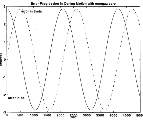
Coning Motions ... 55

Algorithm Error Propagation ... 56

Inertial Algorithm ... 60

Constraints of Buoy Motion ... 60

Complementary Filters ... 60

Model of Wave Motion Caused Angle Error ... 62

Horizontal Reference Frame for Heading ... 64

Inertial Algorithm ... 65

Data Processing ... ... 67

Simulation of Inertial Processing ... 70

General Accuracy Results of Simulations ... 71

Intermediate Reference Frame for Heading ... 72

Rejection of Coning Motion ... 73 6

Low Frequency Errors ... 73

Algorithm Error Breakdown ... 77

Simpler Inertial Algorithms ... 81

Chapter 3. Performance 85 3.A. Modeling Sensor Errors ... 85

3.B. Measurements of Performance ... 94

Electronic Noise ... 95

Electronic Zero Drift ... 96

Sound Speed Changes ... 96

Thermistor Response Time ... ... 96

Bias in Constant Flow ... 97

Wake Error Cancellation ... 97

Measured Bias in Constant Flow ... 99

Variance in Constant Flow ... 102

Bias in Wave Flow ... 105

Rotation Arm Bias ... 106

Wave Bias Sensitivity to Orientation ... 113

Open-Ocean Bias Measurement ... 115

Wave Spectral Rejection of Vorticity Sensors ... 121

Laboratory-Wave Spectral Rejection ... 121

Ocean-Wave Spectral Rejection ... 123

Buoy Flexing ... 124

4.A. Upper-Boundary-Layer Shear ... 129

4.B. Thermocline Richardson Number ... 136

Chapter 5. Summary 139 5.A. Concluding Remarks ... 139

5.B. Future W ork ... 141

Appendix A. Mechanical Drawings ... 142

Appendix B. Processing Code ... ... 152

Appendix C. Rotating Arm Measured Vorticity Bias ... 165

Appendix D. Upper-Boundary-Layer Shear in Wind Coordinates ... 171

LIST OF FIGURES AND TABLES

Fig. 2-20. Block diagram of Euler angle algorithm ...

Page No.

Langmuir cells ... 17

Circulation error from transducer wakes with triangular ... 24

and square geometries Velocity cancellation in constant flow ... ... 25

Photo of 15 cm path vorticity sensor ... .... ... 26

Photo of shear measuring buoy ... 27

Relative beam patterns for transducers ... .. 32

Transducer mounting ... 33

Thermocline shear measuring drifter ... 36

Photo of electronics ... 37

Block diagram of electrical system ... 38

Vorticity meter data format ... 39

Inertial measurement unit sensors ... ... 41

Calibration of accelerometers ... 43

Calibration of rate gyros ... 44

Calibration of Magnetometers ... 45

y axis rate gyro noise ... 46

Inertial sensor noise standard deviations ... 46

Rotation of coordinate system xyz to x'y'z' ... 47

3,2,1 Euler angle system order of rotations ... 49

Coordinate system used in compass example ... 53

Measured heading for rocking buoy ... .... 55

Error progression in coning motion ... .... 59

Complementary filter of redundant sensor measurements ... 61

Conceptual block diagram of inertial processing ... 62

Angle noise for 2D model with Pierson-Moskowitz spectrum .... 64 Pig. 2-1U.

Fig. 2-10.

Fig. 2-21. Vorticity meter data path ... 67

Fig. 2-22. Algorithm to compute earth referenced flow velocity ... 69

Fig. 2-23. Inertial processing simulation block diagram ... 70

Fig. 2-24. East and vertical velocity spectral densities from deployment ... 74

south of Martha's Vineyard Fig. 2-25. Simulated east velocity spectra ... 76

Table 2-4. Array of simulations used to infer size of error terms ... 78

Fig. 2-26. Pole-zero plot for simulated fast sampling ... 80

Table 2-5. Simulations of simpler inertial algorithms ... 82

Fig. 3-1. Geometry of potential flow model ... ... 86

Fig. 3-2. Geometry of wake error models ... 88

Fig. 3-3. Wake model for center stalk and pod wake bias ... 89

Fig. 3-4. Center stalk model used on tow tank data ... 91

Fig. 3-5. Geometry of lift related circulation model ... 93

Fig. 3-6. Current measured in a bucket ... 95

Fig. 3-7. Measured circulation path velocities ... .... 97

Fig. 3-8. Vorticity bias for triangular circulation path ... 99

Fig. 3-9. Uncorrected vorticity bias in constant flow ... 100

Fig. 3-10. Corrected vorticity bias in constant flow ... 100

Table 3-1. Vorticity sensor bias in 0.643 m/sec constant flow ... 101

Fig. 3-11. Geometry used to measure shed vortex wake ... 102

Fig. 3-12. Fluctuating measured velocity perpendicular to center stalk ... 103

Fig. 3-13. Spectral densities of cross and parallel velocities of 45 cm ... 104

path sensor Fig. 3-14. Spectral densities of measured cross velocities at different ... 104

carriage speeds Fig. 3-15. Vorticity means from rotating arm test ... ... 107

Fig. 3-16. Down-wave vorticity means ... 108

Fig. 3-17. Vertical vorticity means ... 108

Fig. 3-19.

Rotating arm sensor means plotted with respect to ...

110

relative drift velocity

Fig. 3-20.

Rotating arm vorticity means for constant ...

111

drift-velocity-divided-by-wave velocity

Fig. 3-21.

Horizontal acceleration spectra from rotating arm test ... 112

Fig. 3-22.

Open-ocean deployment acceleration spectra ... 112

Fig. 3-23.

CCIW wave tank flow measurements ...

113

Table 3-2.

Mean vorticity in tank coordinates at different sensor rotations

...

115

Fig. 3-24.

Mean vorticity measured by shallow sensor south of ...

116

Martha's Vineyard

Fig. 3-25.

Mean vorticity measured by deep sensor south of ...

116

Martha's Vineyard

Fig. 3-26.

Directional wave spectrum south of Martha's Vineyard ... 117

Fig. 3-27.

Coordinate rotation to wave coordinates ...

117

Table 3-3.

Mean vorticity in wave coordinates ...

118

Fig. 3-28.

Vertical vorticity in buoy heading bins ...

119

Fig. 3-29.

Horizontal vorticity in buoy heading bins ...

120

Fig. 3-30.

Wave tank time series of velocity, shear, and circulation over ... 121

path length

Fig. 3-31.

Vorticity meter spectral rejection of waves ...

122

Fig. 3-32.

1.5 m path benthic vorticity meter spectral rejection of waves .... 123

Fig. 3-33.

Measured spectral density of velocity ...

...

125

Fig. 3-34.

Enlarged view of measured spectral peak ...

125

Table 3-4.

Major sensor error sources ...

127

Fig. 4-1.

_{Buzzards Bay deployment shears, measured and estimated from .. 130}

wind stress

Fig. 4-2.

Vertical velocity spectra from Buzzards Bay ...

131

Fig. 4-3.

Buzzards Bay deployment gradient Richardson numbers ... 132

Fig. 4-4.

_{Wave velocity directional spectrum from Buzzards Bay ...}

₁₃₃

Fig. 4-6.

Vorticity from deep sensor in Buzzards Bay ... 135

Fig. 4-7.

Massachusetts bay thermocline gradient Richardson numbers ....

137

Fig. 4-8.

Histogram of Richardson numbers measured over two length scales 138

Fig. A-1.

Shear measuring buoy assembly ...

143

Fig. A-2.

Vorticity sensor assembly ...

144

Fig. A-3.

Pressure vessel assembly ...

145

Fig. A-4.

Lower hub detail ...

146

Fig. A-5.

Upper hub detail ...

147

Fig. A-6.

Custom end cap detail ...

148

Fig. A-7.

Instrument electronics case detail ... ... . 149

Fig. A-8.

Transducer mount detail ...

150

Fig. A-9.

Central stalk, pod arms, and braising jig ... .. 151

Table B-1.

Data Variables ...

152

Fig. C-1.

Vorticity means in constant flow ...

166

Fig. C-2.

Vorticity means at 10 second rotation ... 167

Fig. C-3.

Vorticity means at 7 second rotation ...

167

Fig. C-4.

Vorticity means at 5 second rotation ... ....

168

Fig. C-5.

Vorticity means at 3.8 second rotation ... ... 168

Fig. C-6.

Vorticity means of 15-cm path sensor ...

169

Fig. C-7.

Buoy response functions ... 170

Fig. D-1.

Windstress coordinate system ...

171

Table D-1.

Santala upper-boundary-layer shear model ... 172

Fig. D-2.

Santala model layer transition depths ... ...

173

Fig. D-3.

Downwind shear from vorticity and windstress 0.83 m depth ....

174

Fig. D-4.

Downwind shear from vorticity and windstress 2.45 m depth ....

174

Fig. D-5.

Stratification in lower sensor and between sensors ... 175

CHAPTER 1. INTRODUCTION

This thesis documents the development and testing of an instrument system to measure ocean vorticity and shear in the upper, internal, and bottom-boundary layers. The purpose of this project has been to provide ocean scientists with a tool capable of

measuring ocean shear with finer resolution and or closer to the boundaries. The deployment data are presented to demonstrate the instrument's potential rather than to contribute directly to understanding marine boundary layers.

This chapter describes the geophysical environment to be measured, why vorticity is used to measure shear, how shear can be used to measure vertical diffusivity, and reviews the tradeoff between resolution and accuracy in a shear or vorticity measurement. The upper-boundary layer, internal-boundary layer, and bottom-boundary layer are reviewed to motivate their measurement and to define the instrument design goals. Chapter two describes the mechanical design, electrical design, the inertial measurement unit and its inertial processing, and the signal processing done on the raw data. Chapter three models and measures the sensor performance. Chapter four describes two

deployments of the instrument: one in the upper boundary layer to measure shear, and one in the thermocline to measure gradient Richardson number. Chapter five concludes the thesis and discusses future work and improvements to the system.

L.A. OCEAN BOUNDARY LAYERS

Boundary layers mediate the turbulent fluxes of heat, momentum and chemical species. Turbulent transport dominates molecular diffusion everywhere except in diffusive sublayers on the order of one millimeter thick. The water side of the air-sea interface controls the air-sea transfer of most gasses (Kitaigorodskii and Donelan, 1984). Gas transfer resistance is a function of turbulence in the boundary layer. Many quantities in ocean boundary layers such as Reynolds stress, chemical flux, or shear are difficult to measure in the presence of gravity-wave velocities that swamp turbulent velocities.

Typical boundary-layer flows have wave velocities of order 0.5 m/s and shear of order 2 * 10-2 per second. Over large measurement separations ie. ten meters, this shear is readily measured. Yet over 0.5 meters, if the shear is to be measured with current meters, the meter's accuracy would need to be better than one percent. In the presence of waves this accuracy is not readily achievable. This difficulty results in a shortage of near-surface measurements of shear and poorly-calibrated-closure relations for ocean and climate models. Vorticity can be measured as a surrogate for shear because time-average, area-average, horizontal vorticity equals time-area-average, area-area-average, vertical shear in ocean-boundary layers. A nonintrusive measurement of vorticity would measure wind-driven shear and automatically remove irrotational surface-gravity-wave and current velocities, allowing measurement of shear.

This thesis will emphasize measurements for studies of vertical diffusivity. For readers not too familiar with geophysical flows, vertical (diapycnal) diffusivity is orders of magnitude smaller than horizontal (isopycnal) diffusivity. In the open ocean, far away from boundaries, a typical horizontal diffusivity is 3 m2 _{/s while the vertical diffusivity is}

just 1*10-5 m2 _{/s (Ledwell, Watson, and Law, 1993). Density structure clearly plays a}

large role in ocean diffusivity.

UPPER-BOUNDARY LAYER

The measurement of upper-boundary-layer shear is the focus of this instrument development. The ocean-upper-boundary layer is often compared to the well studied and relatively well understood unstratified turbulent flow over a rigid wall. Factors that can complicate the ocean surface are waves, wave breaking, stratification, rotation, and organized motions such as Langmuir cells.

Shear in a constant stress layer in an unstratified turbulent flow next to a rigid wall, is given by equation (1-1) for distances greater than -- >50 from the wall, of order 5 mm

V

au

.

in the ocean (Morniand Yaglom, 1987). In this equation, -- is Eulerian shear, u.is the

friction velocity _{C the square root of the shear stress divided by density,}

au _- U. _(1-1)

az

KZ

K is von Karmon's constant usually assumed to be 0.4, and z is the distance from the wall.

This shear will give a logarithmic velocity profile, equation (1-2), and the dissipation will

u

u(z) = I--ln(z) + const. (1-2)

K 3

be -- (Tennekes and Lumley, 1989). The assumptions for this log layer are constant

KZ

shear stress, constant density and a Reynolds number high enough that viscous forces are negligible compared to turbulent Reynolds stress. By comparing measured ocean shear to measured windstress, the effects on vertical mixing effectiveness of stratification, wave breaking, surfactants, and Langmuir cells can be measured.

Stratification can inhibit turbulence. To show how this happens, the turbulent kinetic energy budget equation will be reviewed, equation (1-3) (Stull, 1988). In this

a

a

at

x

z

z

a

P

2

po

term: (a) (b) (c) (d) (e)

(

equation, term a is the material derivative of turbulent kinetic energy q,2=u ,2 +v 2 +,2 term b is creation of turbulent energy by shear, term c is pressure diffusion, term d is energy diffusion, term e is viscous dissipation, and termf is destruction by buoyancy. In a steady-state, horizontally-uniform, boundary layer, term a is assumed zero and the

transport terms c and d are assumed very small leaving equation (1-4). The energy destruction-by-buoyancy term takes energy away from turbulence.

-u PO+ (1-4)

8z p₀

The wind driven current as a function of depth is a function of the vertical-eddy diffusivity, which in turn is strongly influenced by stratification (Price, Weller, and Schudlich, 1987). If a constant wind stress and a constant vertical-eddy diffusivity with depth is assumed, the momentum balance, including Coriolis force, generates an Ekman spiral. If eddy diffusivity is assumed to be proportional to depth, a different result is obtained which is closer to most ocean measurements of current shear (Madsen, 1977). The solution is a function of the vertical eddy diffusivity, which in turn is a function of stratification and any other modifications to the turbulence such as wave breaking energy addition, or Langmuir cells. The instrument developed in this thesis measures shears close to the ocean surface, in the upper three meters, where there are few shear measurements.

FREE SURFACE CONSIDERATIONS

Free-surface considerations that can be important to understanding the ocean-upper-boundary layer include Langmuir cells, a reduced-shear layer (as compared to the turbulent wall layer model), gas transfer, wave breaking and their resultant bubbles and

droplets, and surfactants.

Langmuir cells are three-dimensional drift currents that form counter-rotating helical vortices parallel to the wind, Fig 1-1 (Langmuir, 1938). Langmuir cells are often identified by windrows of debris floating parallel to the wind, and arranged by

convergence zones of the vortices. When these cells exist, they dominate vertical mixing over their extent (Gordon, 1970). While cell-averaged shears are of order 1 x 10-2/s, shear is concentrated on the edges of the down welling jets and can be significant compared to average current shear. Langmuir cells are important in understanding the upper-boundary-layer dynamics and complicate measurements in this environment by making time-average

Figure 1-1. Artists conception of Langmuir cells

The transfer of momentum from wind to waves and current is not well understood

and is an area of active research. While the wind's momentum is transferred initially

largely to waves, and most of this to short wavelets, most of this momentum is

transferred through breaking to Eulerian shear and currents. Less than six percent of the

transferred momentum eventually is radiated away as waves (Mitsuyasu, 1985). Many

researchers have found a layer of reduced shear and enhanced dissipation (some by a

factor of 100) as compared to a wall layer (Csanady, 1983 and 1984, Cheung and Street,

1988 a and b, Agrawal et al, 1992). Santala (1991) reports a zone of no shear in the

direction of windstress to a depth of gz

1.2

*

105 and significant shear at right

2

angles to the windstress . One of the guas in developing the vorticity meter is to be able

to make better open-ocean measurements of shear close enough to the surface to study

this reduced shear phenomenon.

Research on gas transfer between the ocean and atmosphere has received increased interest with the concern over atmospheric carbon dioxide buildup. The transfer of low-solubility gases is controlled by the water-side diffusive sublayer, which is of order one millimeter thick (Kitaigorodskii and Donelan, 1984). Straining and renewal of the diffusive sublayer by upper-boundary-layer turbulence is a major contributor to gas

transfer (Brumley and Jirka, 1988). Bubbles from wave breaking can significantly increase gas transfer when the wind exceeds some velocity (Broecker and Siems, 1984). In

addition to their increased effective-surface area for diffusion, bubbles add turbulence and strain the diffusive sublayer.

The presence of surfactants affect the surface boundary condition, dampen capillary waves, and reduce gas transfer (Hunt, 1984). While surfactants reduce the surface drag coefficient, Wu (1983) reports that surfactants can still increase surface drift currents.

SENSOR- WA VE-CORRELA TION BIAS

Sensor-wave-correlation bias of velocity and velocity-derived-shear measurements is caused by a correlation between sensor motion and the wave-field-velocity gradient (Pollard, 1973). It is different from Stokes drift and Stokes-drift shear because sensors and buoys do not exactly follow water motion. In open-ocean fetch conditions, this bias is greater than wind-driven Eulerian shear (Wu, 1975). Santala (1991) and Santala and

Terray (1992) derived an algorithm for removing this bias from measurements taken from

an inertially instrumented buoy, but the accuracy of this bias removal is limited by the

accuracy of the measurements of the directional-wave spectrum. A nonintrusive

measurement of vorticity, on the other hand, is not effected by any motion-correlation

bias.

REASONS TO MEASURE EULERIAN SHEAR

In addition to measuring Eulerian shear to understand the structure of surface boundary layers, one reason for measuring Eulerian shear is to be able to determine the

effective turbulent diffusivity. Comparing wind stress to Eulerian shear results in a measurement of the vertical-eddy diffusivity, and by the Reynolds analogy for turbulent diffusion, is also a measurement of the effectiveness of turbulent transfer of heat and solutes (Rohsenow and Choi, 1961). This measurement of turbulence, although indirect, is better conditioned than direct measurements of Reynolds stress near the ocean surface because of the very large quadrature components from wave velocities that do not contribute to the vertical flux of momentum, heat or solutes. Any wave reflections (standing waves) or phase lag between velocity measurement axes, dooms a measurement of Reynolds flux in the wave field.

MEASUREMENT TYPES

Different methods for measuring drift currents and shear include Lagrangian drifters, Eulerian measurements, and surface-referenced buoys. For measuring mass transport velocities, Lagrangian drifters seem like an obvious inexpensive option. The problems with drifters include uncalibrated drift relative to their target depth (Geyer,

1989), and their tendency to get stuck in convergence zones of three-dimensional flow structures such as Langmuir cells, which can have unrepresentative drift velocities. If measurement of Eulerian shear is desired, the correlation bias of sensor-wave motion of the drifters would have to be compensated for, which would require inertial

instrumentation and measuring relative velocity, significantly increasing the drifter's cost and complexity. An Eulerian (fixed in space) measurement of velocity or shear requires a tower which is expensive, has a large flow obstruction, and cannot be used in deep water. Three-point moorings and taut moorings are not stiff enough to make Eulerian-velocity measurements free of motion-correlation bias. Surface-referenced buoys are often used to measure ocean currents but buoy motion must be known in order to remove wave bias (Santala, 1991 and Santala and Terray, 1992). Buoys ride with swell, giving a

non-Eulerian reference frame. This swell-based reference frame can actually assist near-surface measurements, allowing velocity measurements within a waveheight of the surface

(Cheung and Street, 1988). Measuring vorticity from a surface buoy avoids motion-correlation bias, but the buoy must be inertially instrumented to remove buoy motion from

the buoy's measurements. If the buoy motion is not known and not compensated for,

motions such as coning motions could result in time average sensor measurements that are

caused by the buoy motion and do not exist in the fluid. Coning motions will be explained

in the inertial processing section.

INTERNAL BOUNDARY LAYER

Density-stratified layers in the ocean inhibit turbulent-vertical mixing, support

internal waves, and can be treated as a boundary layer (Salmon, 1990). The gradient

Richardson number equation (1-5) is a ratio of the relative strengths of stratification,

_ dPr

N

_{p dz}

Ri (1-5)

dU )2 dU)

dz dz

which inhibits mixing, and shear, which encourages mixing (Turner, 1973). In this

dU

equation, N is the Brunt-Vaisala frequency, - is the vertical shear, g is gravity, po is

dp,

dz

average density, and

is the density gradient. A gradient Richardson number less than

dz

one quarter is a necessary, and in practice usually sufficient, condition for turbulent

vertical mixing to occur. Internal waves have vorticity in a density-stratified layer.

Internal-wave-shear instability is thought to be the major source of vertical mixing in

density-stratified layers of the ocean away from boundaries; therefore accumulating more

gradient-Richardson-number statistics in the ocean over different spatial scales will help in

further understanding vertical mixing in the ocean (Gargett et al, 1981, and Gargett and

Holloway, 1984).

BOTTOM-BOUNDARY LAYER

Understanding turbulent transport and stress in the bottom-boundary layer is

necessary to understand processes of sediment transport. Measurement of

bottom-boundary-layer turbulence near shore is complicated by surface wave swell that reaches

the bottom, is often much more energetic than the turbulence, and occupies the same

frequency band (Grant and Madsen, 1986). The ability to measure turbulence, free of

surface swell, should assist ocean scientists in studying nonlinear wave-current interaction.

By measuring vorticity, the surface swell is filtered out leaving the turbulence to be more

readily measured.

1.B. PREVIOUS WORK

Other researchers have made single-axis vorticity measurements in laboratories and in the ocean. Rossby (1975) proposed measuring ocean vorticity and made a laboratory demonstration of single axis vorticity measurement by measuring the circulation around a closed triangle by measuring the difference in acoustic travel time. The lab demonstration used acoustic mirrors to form the circulation triangle. He proposed measuring circulation around a large triangle of from 3 kilometers on a side to ocean-basin size. Tsinober, Kit, and Teitel (1986) measured single-axis vorticity electromagnetically in a lab over very small scale. They made a seven electrode probe to make a central difference

approximation of the divergence of the electric potential which is proportional to fluid vorticity. Their probe was only 2 millimeters across. Muller, Lien, and Williams (1988) estimated relative vorticity in the ocean from current meters that were trimoored in the ocean thermocline. The current meters formed horizontal triangles from 8.5 to 1600 meters on a side and the measurements were not compensated for mooring motion. Menemenlis and Farmer (1992) measured vertical vorticity 8 and 20 meters beneath the arctic ice sheet acoustically. They measured circulation around a triangle 200 meters on a side. Tom Sanford (APLUW, personal communication) has measured small-scale, single-axis vorticity in ocean boundary layers by measuring the divergence of the electric field. The instrument whose development is described in this thesis, has made the first three-axis vorticity measurements in ocean boundary layers.

1.C. INSTRUMENT DESIGN GOALS

Eulerian shear in the ocean-upper-boundary-layer, over finer resolution and closer to the surface, than previously practical. The system should be deployable by a moderately sized oceanographic vessel such as the R. V Asterias (a 15 meter workboat), and the

measurement volumes should be scaled and at a depth to measure the reduced shear layer. Below a depth of about 5 meters, moored current meters are adequate for measuring shear. This instrument measures shear in the upper 5 meters of the ocean and can measure shear in the upper meter of the ocean in order to measure the reduced shear layer. A secondary goal for the system is that it be able to measure internal-wave shear and

stratification in the internal-boundary layer (thermocline) over small scales in the presence of surface swell. An ancillary use for these sensors was to measure turbulence in the bottom-boundary layer in the presence of surface swell. This later application of the vorticity meter is not covered in detail in this thesis, but data from this application is presented to show swell-spectral rejection in a coastal deployment.

CHAPTER 2. INSTRUMENT DESIGN

Chapter two describes several aspects of the mechanical design, electrical design, and signal processing. The signal processing section reviews the calculation of instrument attitude and motion in inertial space, develops an algorithm that can use inexpensive low-power sensors to measure instrument motion, describes the data processing done on all the raw signals, and simulates the inertial processing. The inertial simulations show that when using this inertial algorithm, errors in measuring vorticity and shear resulting from imperfect knowledge of buoy motion, are much smaller than errors resulting from flow disturbance. Readers not interested in inertial processing can skip the signal processing subsections, except the data processing subsection, and still follow the rest of the thesis.

2.A. MECHANICAL DESIGN OVERVIEW

In this instrument, circulation around a closed square path is measured, which via Stokes theorem, is the area-integrated vorticity over the surrounded area, equation (2-1).

fA

dA

_(2-1)

• = Vx V

In this equation V'is velocity, Wis vorticity and I is circulation. Vorticity is the curl of the velocity field. The z-direction vertical shear of a horizontal x-directed velocity

corresponds to a vorticity in the y-direction. A square was chosen for the circulation path to minimize disturbance to circulation in a constant mean flow. A triangle has fewer paths, but as Fig. 2-1 shows, a mean current could produce a wake on one side that would generate a significant measured circulation where one did not exist in the undisturbed flow. The wakes resulting from a symmetrical square of transducers largely cancel out, minimizing the vorticity error due to wakes.

The water velocity in each path around the square is measured acoustically. Differential acoustic travel times on each path are measured by modified Benthic Acoustic

Fig. 2-1 Circulation error from transducer wakes largely cancel out with a square geometry but not with a triangular geometry.

Stress Sensor (BASS) electronics (Williams et al, 1987). The water velocity v parallel to each acoustic path is given by equation (2-2) where c is the speed of sound, at is the

C2ad 2)

2L C2

differential travel time, and L is a single, acoustic-path length making up one side of a square. BASS electronics were chosen to measure velocity because of their speed, accuracy, and low noise; single-pulse time noise is forty picoseconds. The option of using acoustic mirrors and fewer transducers was dismissed due to problems in distinguishing the signal from reflections off the structure.

divided by path length (Fig. 2-2). Circulation divided by path length is plotted instead of true circulation or vorticity, because it has the same units as velocity so that cancellation

Velocities Around the Square

50

-50 I 2 0 0

S0

10 20 30 roulatio nathle 60th 70 80 90 100

0 10 20 30 40 50 60 70 80 90 100

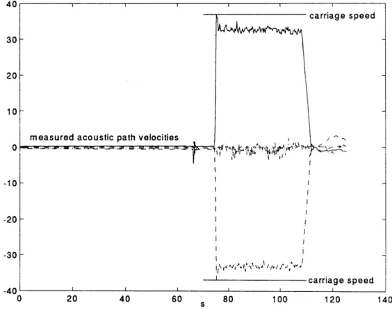
Fig. 2-2. Results from a typical tow tank run showing measured velocity from each acoustic path around the square, circulation divided by path length, and vorticity. This sensor was at an angle to the flow.

of antiparallel velocities can be evaluated. The prototype lab vorticity meter, when oriented with two of the acoustic paths parallel to the flow, (the worst orientation for velocity measurement) measured ten percent less velocity than the undisturbed flow. Parallel paths, however, have the same decrement to within one percent, resulting in small vorticity error.

A three-axis vorticity sensor was designed to minimize wake-related errors when buoy deployed. For an instrument to be deployed on an ocean buoy, all three axes of

vorticity have to be measured because buoy attitude can change. Buoy motion can then be compensated for, in signal processing, if the buoy's motion is known. A prototype

vorticity meter with 15 centimeter acoustic paths was made and is shown in Fig. 2-3. The

Fig. 2-3. Photo of the prototype three-axis vorticity meter with 15 paths.

cm acoustic

15 centimeter path length was chosen for convenience in the lab and compatibility with

existing electronics. Twelve acoustic paths form the edges of a regular octahedron and

form three, orthogonal, circulation path squares. Each sphere contains four piezoelectric

transducers that form the corner of two circulation path squares. Because a flow sensor

mounted on a buoy may measure flow in any direction, but cannot be streamlined in all

directions, the design philosophy was to minimize wake asymmetries and errors in

circulation. This geometry maximized symmetry and minimized measured circulation flow

disturbance. If some of the parts are streamlined, such as the cylinders, they would

become lifting surfaces when the flow angle of attack changes and create lift-related

circulation, ie., error. Velocity defects symmetric with respect to acoustic circulation

paths, do not contribute significantly to error in measured circulation. This prototype

sensor was tested for bias in uniform flow in tow tanks and wave rejection in a wave tank

with the results of these tests justifying our building several larger versions.

The ratio of circulation signal to wake induced noise is expected to increase with

longer path length so the ocean deployed instruments were scaled up from the prototype.

Two vorticity sensors with

45

centimeter acoustic paths, were built into an inertially

instrumented buoy to measure shear Fig. 2-4. A vorticity sensor with a 1.5 meter acoustic

path length, was built as its own tripod for measuring the turbulent vorticity and shear in the bottom-boundary layer; this sensor will only be briefly commented on in the

performance section where it is used to show spectral rejection of waves during a coastal deployment (Williams, Terray, Thwaites, and Trowbridge, 1994).

The sensor geometry uses a center structural stalk to reduce circulation

disturbance as compared to using a braced frame. A braced frame such as one that BASS uses, has a much better strength and stiffness to weight ratio, and can utilize smaller structural members. Its members are then, however, at a radius from the measurement volume center, and any asymmetry between structural member wakes and acoustic paths would create large circulation disturbances. Tube bending strength is proportional to the tube diameter cubed and bending stiffness to the diameter to the fourth power, while drag and consequent wake size is linear to the tube diameter. If one is looking for strength to drag ratio, a nonbraced larger center tube is not at a disadvantage. An additional benefit of this design is that all the wires are strung inside the tubing and not exposed to

hydrostatic pressure. Hydrostatic pressure applied to cables squeeze the cables and change the cables' capacitance, which can cause instrument zero drift.

The sensor structure was kept smooth to avoid tripping its boundary layer. The Reynolds number for a two-centimeter tube or sphere at one meter per second velocity is about 2 * 10" which is below the laminar-to-turbulent, boundary-layer transition zone. For a sphere, this transition zone Reynolds number ranges from 7 * 104 to 5 * 105 depending on such variables as surface roughness, ambient turbulence, and structural vibration (Potter and Foss, 1982).

One drawback of this octahedron design is a lack of redundancy. If any of the twelve acoustic paths fails on a buoy deployment, there will be no earth-referenced vorticity without using the questionable assumption of zero correlation between buoy attitude and water motion. This lack of redundancy could only be solved with a substantial increase in flow disturbance.

VORTEX SHEDDING

Any bluff body (at these Reynolds numbers) moving with respect to a fluid has oscillatory forces exerted on it by the fluid which are associated with the body's von Karmon vortex street. Acoustic current meters are sensitive to instrument strumming. The largest oscillatory force on a tube is perpendicular to both the tube and the flow

direction, at a frequency given by equation (2-3) (Blevins, 1977). In this equationf, is the

SU

f D (2-3)

S

=

0.2

frequency of the periodic forcing, S is the Strouhal number, U is the relative velocity, and

D is the body diameter. Vibration can have a strong organizing effect on the von Karmon

wake, which increases the lateral force exciting the structure, and can cause lock-in of lightly-damped structures. In addition to the large lateral exciting force just described, there is a smaller oscillating force parallel to the flow at twice the frequency given above that can cause lightly damped structures to lock-in at this higher Strouhal number

(Crandall, Vigander, and March, 1975). The braised stainless steel structure of the vorticity meter has very little damping, so that strumming has to be considered.

The prototype with the 15-centimeter path, showed no problems with strumming. The first natural frequency of the pod arms was measured to be 123 Hz and that of the center stalk to be 28 Hz. The pod arms had polyurethane injected into the annulus

between the wires and the tube interiors. While this did not effectively add damping, it did keep the cables from rattling around and acted as a pressure block. Smaller structures naturally have higher natural frequencies than larger structures.

The vorticity sensors with the 45 centimeter acoustic paths, were designed with thin pod arms for minimum flow disturbance. The pod arms vibrate at 30 Hz with a damping ratio of only 0.00038, measured with the logarithmic decrement method over

1,800 cycles (Meirovitch, 1975). In a constant flow, the first strumming occurs at 70 cm/s

and is in the double frequency parallel mode. As mentioned previously, the buoy that

these sensors form, was designed to ride with ocean swell. In the open ocean

deployments the relative velocity between the sensors and water has never been this large

so strumming has not been a problem.

As an additional project, two more 45-centimeter path, vorticity sensors were built

to measure bottom-boundary-layer turbulence in high tidal currents. The design changes

for these sensors will be discussed as well. The solution we chose was to raise the pod

arms' natural frequency and damping by adding pipes that were half as long as the pod

arms, screwing them into the center stalk, and filling the annulus between the pod arms

and pipe with polyurethane resin. Polyurethanes have high damping and are often used to

absorb vibration energy. The resulting natural frequency of the pod arms was doubled and

had high damping. These sensors were tested and observed in Vineyard Sound, MA. in a

two knot tidal current and showed no signs of strumming. In designing this modification,

physical dynamic models were made and tested with polyurethane by itself, fiberglass in

epoxy, carbon in epoxy, and fiberglass in polyurethane, in addition to the double tube filled

with resin. None of the other damping designs were effective at the lower structural

modes of vibration.

MATERIAL SELECTION

The sensor frames are silver-braised, 316 stainless steel while the instrument case

is anodized 6061 aluminum. The silver braise did not corrode in fresh water, but did have

to be protected (in this case by polyurethane) in seawater. Other materials considered but

not chosen included 316L stainless steel, titanium, and carbon fiber. Titanium and 316L

stainless steel were not available in the shapes needed, and titanium cannot be braised

satisfactorily. Gun-barrel drilling all the tubes in this structure would have been too

expensive. The instrument, in general, was designed for "one off' manufacturability with

all shapes machinable using standard cutters, and all material available from stock sizes.

Carbon fiber was not used because of its cost and in this application provided marginal advantages. Carbon fiber structures, when at least vacuum bagged during curing, have better strength-to-weight ratios and much better stiffness-to-weight ratios than metal; however, to achieve this level of performance requires all the excess resin to be squeezed out. This necessitates the molds to be "two and a half' dimensional in that they must have one surface that moves as the excess resin is removed. This reduces design flexibility. High-strength carbon structures have to be carefully designed and laid up because of carbon's brittleness. The primary motive in considering the use of carbon was to increase structural natural frequencies, to push up the minimum velocity of strumming. In air wherein added mass is negligible, carbon fiber structures can be very competitive; but in water the large added mass lowers the natural frequencies to where they would be if the structure was made of metal. The one structural quality of composite structures that is still desirable is their larger structural damping than metal. However, as the strength of a composite material improves, its damping is reduced. Carbon's small additional structural damping did not justify its significantly higher cost.

TRANSDUCERS AND THEIR MOUNTING

The vorticity meter uses piezoceramic transducers to transmit and receive sound waves at 1.75 MHZ. The piezoceramic used was Transducer Products LTZ-2.

Specifications for alignment accuracy can be derived from modeling the transducer as a vibrating piston in an infinite plane wall (Dowling and Ffowcs Williams, 1983). This model gives a pressure at a point given by equation (2-4) where p' is the acoustic pressure,

i2 a sin 0

p ihZ 2Uo io(t- ) 2J c

P '(It) =- e _(2-4)

2R wa sin 0

C

po is the density, o _{is the frequency, a is the transducer radius,} Uo is the velocity of transducer surface, R is the distance to point where the pressure is calculated, J, is the Bessel function of the order one, and c is the speed of sound. The relative beam patterns

for 0.25 inch (0.63 cm) and 0.375 inch (0.953 cm) diameter transducers are shown in Fig.

2-5. The half-power beam width for the 0.375 inch transducers is 2.7 degrees and for the

0.25 inch transducers is 4.1 degrees. These angles correspond to mounting the transducers to the same tolerance of 0.018 inch (0.46 mm). Because of concern for ganging of errors, the final mounting accuracy specification was 0.01 inches (0.25 mm). Alignment of the frame was achieved during braising by attaching a jig consisting of steel rods that were screwed in each acoustic path and fitting all the joints loosely. This technique avoided ganging of errors from all the joints.

The transducers were mounted in polyurethane resin on a stainless steel backbone as shown in Fig. 2-6. The polyurethane used was Conap brand EN-4; we chose it because it is acoustically transparent in water. Insulating the transducers from the steel is a spacer

0 5 10 15 20 25

degrees off center

Fig. 2-5. Relative beam patterns for 0.25 inch (0.635 cm) and 0.375 inch (0.953 cm) transducers at 1.75 MHZ calculated from eqn (2-4).

of Dacron in polyurethane, which was found to meet the alignment accuracy needed. The thin Dacron cloth was never fully saturated by the resin, leaving microscopic air bubbles behind the transducers, but this did not cause any measurable problems. The only stainless

steel-to-urethane primer found to be effective in seawater was Conap brand AD-6, which has an acid base. If water diffuses through the polyurethane jacket, dissolves the acid residue, and migrates to the transducers; the frit adhering the silver electrodes to the ceramic could be attacked by the acid causing transducer failure. The sensors have been left in freshwater for several months at a time with no degradation, but this potential problem should be monitored on long-term deployments. The entire pod is encapsulated in one-sixteenth of an inch of polyurethane.

etec t rode

transducer

spacer of dacron saturated with polyurethane

molded polyurethane stainless steel backbone

Fig. 2-6. Transducer mounting on stainless steel backbone

Piezoceramic transducers have a high acoustic impedance relative to water,

causing a low acoustic transmission coefficient of about 0.04. Quarter wave plates with

an acoustic impedance equal to the geometric mean between that of water and ceramic

were considered to improve the transducer effectiveness, but their additional cost of over

this option unattractive. Instead, the BASS electronics take advantage of the high

transducer

Q

and transmit fifteen cycles of the carrier wave at the transducer natural

frequency. The BASS circuit times off the fifteenth cycle of the receiver transducer,

whose energy is coherently summed from the fifteen cycles. This technique largely

overcomes the low transducer acoustic match with water.

The minimum pod size was set by transducer considerations. Transducers smaller

than 0.25 inch in diameter (0.64 cm) lose much of their effectiveness due to the solder

mass connecting the electrode, thereby detuning that area of the transducer and the

depolarized zone underneath the solder. BASS electronics use a low-input-impedance

cascode receiver to reduce zero drift from cable capacitance change, but this low-input

impedance coupled with the high transducer output impedance requires a strong output

signal from the receiving transducer.

The 15 centimeter path prototype vorticity meter used 0.25 inch (0.64 cm)

diameter transducers; these are the smallest available with both wires attached to one side

of the transducer. The transducer output gain scales as the diameter to the fourth power,

requiring that its transmitter voltage be raised relative to a regular BASS. The prototype

also used EN-4 polyurethane as a pressure block. This is not a hard polyurethane and

could cold flow on a long, deep deployment. These pods ended up having a 1.0 inch (2.54

cm) outer diameter.

The 45 centimeter path vorticity sensors used 0.375 inch (0.953 cm) diameter

transducers to avoid excessive transmitter voltages. The acoustic energy from the receiver

transducer scales as one over the path length squared. The electronics of this instrument

used a three-to-one turns ratio in the toroidal core transformers that power the transducers

(Williams et al, 1987). In these sensors, thermistors (Yellow Springs Instrument Co.

44030) were mounted inside the pod arm tubes at a distance of 2 inches (5 cm) from the

pods on each side of each sensor. The thermistors measure temperature and temperature

stratification. For greater depth capability, the transducer pods use glass-filled epoxy

pressure blocks. These pods have a 1.25 inch (3.17 cm) outer diameter.

The 1.5 meter path vorticity meter briefly mentioned uses 0.75 inch (1.9 cm) diameter transducers and operates at the lower frequency of 875 KHz to keep transducer alignment from becoming too difficult; it is difficult to align objects to less than one degree.

BUOY DESIGN

A shear measuring buoy was built of two 45-centimeter path, vorticity sensors, their electronics, an inertial measurement unit, and a float with recovery gear, Fig. 2-4. The buoy was designed to minimize flow disturbance in the measurement volumes by moving with ocean swell, minimize surface expression (the float), minimize sensor cylinder size, and locating the electronics package well below the measurement volumes.

Measurement volumes are centered at 0.83 meters and 2.45 meters below the water surface, and the total buoy height is 5.06 meters. The buoy has a strapdown, inertial measurement unit to measure buoy motion and remove it from relative flow, and to rotate the measurements into an Earth reference system. The inertial measurement unit is described in the electrical design section and the inertial processing is described in the signal processing section.

The buoy is modular and is bolted together with interchangeable sensors. A bumper of rolled, welded stainless steel tubing is mounted on the instrument case so that the buoy can be laid on its side on a flat surface between this bumper and the top spherical float, and not bend the pod arms. The top float is made of expanded PVC foam with a fiberglass skin. This system is light, relatively incompressible, failsafe, shapable, and corrosion free.

The buoy is deployed freely, drifting with the currents, requiring reliable recovery aids. The recovery systems include an ARGOS transmitter that transmits to a satellite which measures and relays buoy location, a strobe light, a VHF radio transmitter, and

when deployed below the ocean surface, an acoustic transponder that is compatible with a diver-operable, subsea direction finder.

To measure internal wave shear in the thermocline, the buoy can be deployed using an elastic tether between the top float and the rest of the instrument, Fig. 2-7. The drifter uses a bungy cord strung inside a hollow sleeve rope that is slack, to isolate float heave from the instrument. The chain on the float bottom and poly fishnet floats at the

instrument's top keep tension on the elastic tether below two kilograms, allowing a low-spring-rate soft bungy to be used. Observations of the instrument during dives showed very effective heave suppression.

eIastic tether

trawl floats

-- 10 meter depth

Fig. 2-7. Acoustic vorticity meter configured as a thermocline shear measuring drifter.

2.B. ELECTRICAL DESIGN

ELECTRICAL OVERVIEW

Modified BASS electronics (Williams et al, 1987) form the heart of the vorticity meter. The physical electronics, inertial measurement unit and data logger are shown in Fig. 2-8. A block diagram of the electrical system is shown in Fig. 2-9. The BASS

Fig. 2-8. Photo of electronics on right, inertial measurement unit in middle, battery, and data logger at left with the instrument case above.

electronics are controlled by a Tattletale 5 computer made by Onset computers, Pocasset, MA.. The Tattletale 5 computer directs each pair of acoustic transducers to measure water velocity along their acoustic path, polls all the analog inputs from the: thermistors,

accelerometers, rate gyros, and magnetometers; and sends this data serially to a data logger. The data logger is a Tattletale 6 computer that records the data on a hard disk drive after buffering the data in semiconductor memory. This "buffering to memory" is done to save power; the hard disk is only spun up and written to when the memory is fiull. The analog signal conditioning done to the inertial sensors' signals is scaling voltages and

BASS --- - ~ -- -, .1---Piezoceramic Transducers Thermistors Accelerometi Rate Gyros --A/D ' Logger Hard Disk ~~1

Fig. 2-9. Block diagram of electrical system

low-pass, anti-alias filtering. Each of the recovery devices: the ARGOS transmitter, VHF transmitter, and strobe, has its own battery for redundancy. The recovery devices are not shown in this diagram.

One problem with the data logger system is the high current required to spin up the hard disk before a software timeout is reached. The main batteries of this instrument are alkaline which have a high output impedance when cold, and are unable to start the hard disk below a certain temperature. To resolve this problem, a lead acid gel cell with lower output impedance at low temperature, is used as a capacitor to start the disk. This gel cell is then recharged by the alkaline main batteries between disk writes.

The longer acoustic path length required modifying the transmit voltage and timing of the BASS electronics. To increase the transmit voltage, the transformer cores that drive the acoustic transducers were wound with a three-to-one ratio instead of the

one-to-one ratio in a regular BASS. The fast timing to control the acoustic velocity measurement is done in analog on the timing and burst generator card to save power. The instrument transmits fifteen cycles at 1.75 MHz. for 8.57 ps. The receiver is turned on 282.5 pts after the start of the transmit; this corresponds to the fastest measurable sound speed of 1590 m/s. The receiver effectively turns off 344.5 Cps after the transmit start; this corresponds to the slowest measurable sound speed of 1370 m/s. The acoustic path velocity is then remeasured 383.5 gs later with the electronics reversed to cancel out electronic drift. The measurement cycle consists of a time stamp of four bytes, 24 forward and reverse velocity measurements that take 18.4 ms, 13 analog measurements of the thermistors and inertial sensors, and then sending the eighty byte measurement sequence at 9600 baud to the logger, taking 83 ms. The whole measurement sequence is repeated every 150 ms.

The data format is shown in Table 2-1. All the data is transmitted and stored in unsigned binary integers except the velocity measurements which are in two's complement.

EE DD % hexadecimal record header

{ 1 } { 1 } { 1 } { 1 } time % time stamp hr:min:s:counter

{2 } {2 } (2) {2 } podl % four acoustically measured velocities making {2} {2} {2} {2} pod2 % up a circulation square

{2} {2) {2} {2) pod3 %

{2} {2} {2} {2} pod4 %

{2} {2} {2} {2} pod5 %

{2} {2} {2} {2} pod6 %

{2} {2} (2} {2} temp % thermistor output

{2) {2} {2} imul 1% accelerometer

{2} {2} {2) imu2 % rate gyro

{2} {2} {2} imu3 % magnetometer

Table 2-1. Vorticity meter data format. The numbers in brackets indicate the length of each variable in bytes

INERTIAL MEASUREMENT UNIT

A strapdown inertial measurement unit was built into the shear measuring buoy to measure buoy motion allowing the motion to be removed, in processing, from flow measurements. The Inertial Processing Background section shows that it is necessary to measure and compensate for buoy motion even if only time average measurements from a buoy are desired. A strapdown inertial measurement unit was chosen over a gimballed inertial measurement unit to save power and size. A gimballed inertial measurement unit, consisting of accelerometers on a gyro-stabilized platform that does not rotate with respect to inertial space, is more accurate than a strapdown system consisting of the accelerometers, rate gyros and magnetometers mounted "strapped down" to the buoy (VanBronkhorst, 1978). Gimballed systems are expensive, delicate, and consume much power; whereas strapdown systems are inexpensive, more robust mechanically, and consume less power. Strapdown systems do, however, require more computation. Gimballed systems use rate gyros as nulling sensors, do not expose the rate gyros to the angular rates of the buoy, and therefore can measure angular rates more accurately. Strapdown systems, on the other hand, expose their rate gyros to the full angular rates of the buoy, requiring rate gyro accuracy and linearity over a wide range. Gimballed systems are able to cancel out some error terms, such as some small accelerometer misalignment, that strapdown systems can not cancel out (Schmidt, 1978). Some wavebuoys use a low-power version of a gimballed system by floating a large sphere with accelerometers, in oil, and limiting the system's righting response to frequencies lower than the wind-wave spectrum. These wavebuoy systems are however, large and heavy. The shear measuring buoy uses a strapdown inertial measurement unit to save power (battery weight, size, and flow disturbance), to avoid the bulk and weight of some of the wavebuoy inertial

measurement platforms, and to save money.

The strapdown inertial measurement unit consists of a three-axis accelerometer, three single-axis rate gyros, and a three-axis magnetometer. These sensors and some of their specifications are listed in Table 2-2. It is worthwhile to note that these are not inertial-navigation-grade sensors. For example, good inertial grade rate gyros are 10'

Three-axis accelerometer Columbia Triaxial Accelerometer model SA-307 HPTV X -1 to +1 G Y -1 to +1 G Z 0 to +2 G case alignment +/- 0.50

Three single-axis rate gyros Systron Donner Gyrochip Angular Rate Sensor X, Y, and Z -50 to +50 deg/s

bandwidth > 60 Hz. scale calibration 1 %

linearity <0.05% of full scale

input power noise requirement < 0.01 v rms and < 0.001 v rms at 8.7 Khz. +/- 500 Hz. Three-axis magnetometer Develco model 9200 fluxgate magnetometer

X, Y, and Z -600 to +600 mGauss alignment +/- 1l

output ripple 0.4% of full scale

temp stability <3 % from 0°C to 600C sensitivity <1% zero

linearity +/- 0.5% of full scale

Table 2-2. Description of the inertial measurement unit sensors

times more accurate than the low-power rate gyros used in the vorticity meter. The alignment of the sensors used, inside their sensor cages, is only good to about one degree. Techniques such as Schuler tuning are not useful when the rate gyro noise, even when averaged over ten minutes, and drift are ten times the earth's rotation rate. However, with appropriate processing, as is shown in the Inertial Processing section, these sensors are adequate for this application.

The inertial measurement system requirements will now be specified. Errors in estimated buoy attitude and motion should not cause more than five percent error in flow measurements. This translates to an angle error specification of three degrees. Angle rates in sensor coordinates should be better than one percent to compensate for buoy motion. The Inertial Processing Background section shows that the heading specification