Applications of game theory in microgrids

Applications of Game Theory in Microgrids

by

Jie Mei

B.S. in Electrical Engineering

Georgia Institute of Technology, 2015

Submitted to the Department of Electrical Engineering and Computer

Science

in partial fulfillment of the requirements for the degree of

Master of Science in Electrical Engineering and Computer Science

at the

MASSACHUSETTS INSTITUTE OF TECHNOLOGY

June 2018

Massachusetts Institute of Technology. All rights reserved

Auhr..Signature

redacted

A uthor ... ...

Department of Electrical Engineering and Computer Science

May 11, 2018

Certified by..

Signature

redacted...

James L. Kirtley

Professor of Electrical Engineering and Computer Science

Thesis Supervisor

Accepted by...Signature

redacted...

/

J/

(I

Leslie A. Kolodziej ski

Professor of Electrical Engineering and Computer Science

Chair, Department Committee on Graduate Students

OF TECHNOLOGY

Applications of Game Theory in Microgrids

by

Jie Mei

Submitted to the Department of Electrical Engineering and Computer Science on May 15, 2018, in partial fulfillment of the

requirements for the degree of

Master of Science in Electrical Engineering and Computer Science

Abstract

A microgrid, which can be defined as a group of interconnected loads and

distributed energy resources within clearly defined electrical boundaries that acts as a single controllable entity with respect to the grid, has been studied extensively in recent years. This paper will explore the application of non-cooperative game and non-cooperative game in microgrids. For an individual microgrid that is connected with renewable energy sources through DC-DC converters, a non-cooperative game theory based PI controller tuning method is proposed to help make more stable output voltage. For microgrids that are connected in network, a cooperative game theory based local energy exchange scheme is proposed to help them meet their energy requirements while achieving higher individual utility.

Thesis Supervisor: James L. Kirtley

Acknowledgments

First of all, I would like to thank my advisor, Prof.James L. Kirtley. It was him who brought me into the door of scientific research. There is an old Chinese saying called one day a teacher, always a father. I think that what I have learned from him is not limited to scientific research but to all aspects of life, including the harmony with other people, the broad mind like the sea, the love of work, and the love of family members.

Secondly, I would like to thank my parents and my grandmother. Thank you for giving me life so that I can feel the beauty of the world. You are just like the lighthouse on the coast for me. With your light guidelines, I think I will never go the wrong way.

Finally, I want to thank my girlfriend, Xinran Zang. Because of you, I have never thought of giving up even with many difficulties. Because of you, even if I am depressed, as long as I think about the fragments of our stories that are in my mind, I would be happy again. Because of you, I am willing to change myself and become the best of me. May you always be as beautiful as when we first met.

Contents

2. Non-Cooperative Game Theory Based Controller Tuning Method for Microgrid DC-DC Converters... 21

2.1. B ackground ... 2 1 2.2. Multi-objective Optimization of Controller Tuning... 23

2.3. Calculation of Objective Functions... 25

2.4. Game Theory of Controller Tuning... 28

2.5. Sim ulation... 29

3. Cooperative Game Theory Based Local Power Exchange Algorithm for Networked Microgrids ... 35

3.1. B ackground ... 35

3.2. Networked microgrids Model... 37

3.3. Coalition Utility Calculation... 40

3.4. Coalition Utility Allocation and Optimal Coalition Structure ... 45

3.5. Simulation Results and Analysis ... 48

List of Figures

Figure 1. Circuit schematic of a buck converter... 30

Figure 2. Comparison of game theory based tuning method with MATLAB optimal tuning and ziegler-nichols method... 30

Figure 3. Plot of the Pareto Front and Nash Equilibrium point... 33

Figure 4. Traditional m icrogrid system . ... 386

Figure 5. Illustration of networked microgrids system with virtual operator... 408

Figure 6. Stable coalitions of the 13-microgrid network. ... 508

Figure 7. Ratio of average individual incremental utility of moving from non-cooperative to non-cooperative operation and the proportion of power traded between microgrids, for varying numbers of microgrids... 50

Figure 8. Average number of merging-splitting operations and running time of the proposed algorithm with different numbers of microgrids... 51

List of Tables

Table 1. Buck converter parameters ... 31

Table 2. Auction Based Coalition Utility Calculation Algorithm ... 42 Table 3. Parameter selection for simulation ... 46 Table 4. Individual incremental utility and line loss saving for network with 13 m icro g rid s ... 4 9

NOMENCLATURE

Subscript

k Index for member in coalition S

bi Buyer microgrid with microgrid index i

gj Seller microgrid with microgrid indexj

bis, Buyer microgrid with highest bid price

(P k Distributed coalition utility for k

Variables

di Demand power of buyer microgrid b,

ej Excess power of seller microgrid qj

Pio, s Supplied power from transmission substation to meet the power requirement of buyer microgrid b,

Poj, R Received power for transmission substation if seller microgrid qj sells

ej

Pij. s Supplied power from seller microgrid qj to meet the power requirement

of buyer microgrid b,

Pij, snax Maximum amount of supplied power from seller microgrid q1 to buyer

microgrid bi

Py, Rnax Received power for buyer microgrid bi if Pj, smax

are supplied from seller microgrid qj

Pi,, snax Power supplied from transmission substation to make buyer microgrid bi receive Py. Rmax

Poj, Rax Received power for transmission substation if seller microgrid qj sells

Pij, Smax

Pio, L Line losses for buyer microgrid bi to get P,,,s from transmission

P1, L Line losses for seller microgrid qj to sell ej to transmission substation /0] Lowest acceptable bidding price for seller microgrid qj

4

hi The highest price per unit power that buyer microgrid bi is willing to bid in trading with seller microgrid qj

hist Highest bid price in H

h2nd Second highest bid price in H

dis, Demand of buyer microgrid b₁₅,

Parameters

RU; Resistance between seller microgrid qj and buyer microgrid bi

Ro; Resistance between seller microgrid aj and transmission substation

Rio Resistance between buyer microgrid b, and transmission substation

18 Fraction of loss in transformer at transmission substation

Uo Voltage level at transmission substation

U Voltage level at microgrid

0)g Unit electricity price at transmission substation

|SI Number of microgrids in coalition S

jSbj Number of microgrids in coalition Sb

N Number of microgrids in the network

Sets

Gb Buyer microgrids group in a coalition Gs Seller microgrids group in a coalition

D Demand power of microgrids in Gb

E Excess power of microgrids in Gs

N Set of microgrids with N players

S Coalition in cooperative game

1. Introduction

1.1.Motivation

Renewable energy applications will be a feasible solution for energy scarcity and environmental problems as a result of the rapid advancement of global economic growth [1]. However, the distribution characteristics of renewable energy make it difficult to integrate effectively into the traditional power grid. As power networks increase in scale, the drawbacks of the conventional grid, such as high cost and difficult operation, will become more apparent, and it will no longer meet increasing safety, reliability, and diversity needs [2].

In order to integrate renewable energy sources effectively and improve the quality of electric power on the demand side, microgrid, which can be defined as a group of interconnected loads and distributed energy resources within clearly defined electrical boundaries that acts as a single controllable entity with respect to the grid, has been studied extensively. Generally, there are two operating modes for a microgrid: In grid-connected mode, the microgrid exchanges power with the main grid to reduce the variability of renewable energy. In isolated mode, the microgrid is disconnected from the main grid and works autonomously,

balancing its own generation and load [3], [4].

Game theory is derived from economics, but it has also been widely used in social, military, and engineering fields. For more than half a century since its birth, game theory has exerted an important influence on economics and even the entire social sciences, and has become an important decision analysis tool. With the development of microgrids, major changes have taken place in many forms of traditional power systems such as structure, operation, dispatch, and control. On the microgrid power generation side, small-scale wind and solar power generate uncertainties in power supply output. On the demand side, small-scale loads

increase the operational complexity while increasing flexibility. The increasing popularity of electric vehicles and smart homes has made the load more proactive.

If the various types of microgrid energy storage systems are further considered,

the decision-making agents of the system will be more diversified. In this context, how to determine the best strategy for each decision-making agent to optimize and balance the interest conflicts within a microgrid and among neighbor microgrids is a challenging task. However, the traditional theory of deterministic optimization based on single subject decision-making is difficult to overcome this difficulty. Under this background, game theory for multi-objective optimization of complex subjects can be expected to be a powerful tool to overcome many key decision problems in microgrid.

The so-called game is a process in which multiple decision-making agents face certain environmental conditions, and under certain static or dynamic constraints, rely on the information that the decision-makers possess, and obtain the maximum utility by choosing optimal strategies from their feasible strategy sets. Game theory can be broadly divided into non-cooperative games and cooperative games. The non-cooperative game is represented by the work of John Nash. Nash proved the existence of non-cooperative game solutions under certain conditions, namely the existence of the well-known Nash equilibrium, thus establishing the theoretical foundation for modern non-cooperative games. The cooperative game created by von Neumann mainly has two aspects of research: first, how each agent achieves cooperation; second, how each agent allocates additional income due to mutual cooperation. Whether to choose cooperation game or non-cooperation game depends on the characteristics of the problem itself. Human-controlled economic situations generally apply cooperative games to achieve greater benefits. The related problems determined by the characteristics of the system or nature, such as the PI controllers tuning problem which will be mentioned later, generally apply non-cooperative games.

1.2. Contribution

This research will explore the application of non-cooperative game and cooperative game in microgrids. For an individual microgrid that is connected with renewable energy source through DC-DC converters, a non-cooperative game theory based PI controller tuning method is proposed to help get more stable output voltage. For microgrids that are connected in network, a cooperative game theory based local energy exchange scheme is proposed to help them meet their energy requirements while achieve higher individual utility.

1.3.Thesis Structure

The remaining thesis is organized as follows. The non-cooperative game theory based PI controller tuning method will be introduced in Chapter 2. In Chapter 3, the cooperative game-theory-based local power exchange algorithm for networked microgrids will be explained. Finally, Chapter 4 will give the conclusion and future work.

2. Non-Cooperative Game Theory Based

Controller Tuning Method for Microgrid

DC-DC Converters

2.1. Background

As more and more renewable energy sources, such as wind and solar power, are integrated to Micro-grids, fully controllable synchronous generators, which are normally responsible for voltage and frequency control in traditional power systems, become less common in Micro-grids. Those installed micro-sources, including Energy Storage, are not suitable for direct connection to Micro-grids due to their voltage level and other electricity characteristics. Thus power electronics interfaces (DC-DC or DC-AC) are essential in Micro-grid design. Control methods for these power electronic devices are important, as inevitable disturbances include variations and uncertainties from source, load, and circuit parameters can cause circuit operation to deviate from nominal. One fairly satisfactory and widely used control solution in Micro-grids to counteract departures from nominal is based on proportional-integral (PI) controller. The technical community shows continued interest in new tuning methods for finding optimal control parameters for the proportion and integration parts [5].

PI controller tuning can be viewed as the search for the best compromise between all the specifications and thereby many researchers applied the idea of multi-objective optimization as an alternative to resolve this problem [6]. Solving the multi-objective optimization can yield a set of solutions in which no objective can be improved without sacrificing at least one other objective. Graphically, this

is often expressed as the 'Pareto Frontier'. The problem is how to choose the final solution among the Pareto set, since no solution is better according to multi-objective optimization definition. In another words, much decision choices in turn makes it difficult to make a decision. In reality, many of the objectives in the multi-objective optimization are conflicting. Thus how to meet all the objectives and show the importance of every objective, in another words, make final decision among elements of the Pareto set, is the core part of the multi-objective optimization, which has been studied for many years. Traditionally, there are generally two groups of methods to solve the problems. The first method is to set a single-objective evaluation function and using weighting factors to show the importance of every objective thus transferring multi-objective optimization to a single-objective optimization. The other group of methods uses the techniques of layering, grouping, and classifying methods to change multi-objective optimization to single-objective optimization. For those methods, the optimum of the weighted single objective depends on the preference of the designer a lot and thus lacks objectivity [7]. In fact, when a designer is making decision among conflicting objectives, the ultimate goal is to reconcile the conflict. Thus, a theory to reconcile the conflict between objectives is needed to avoid subjective arbitrariness. In this context, using Game Theory to solve multi-objective optimization seems rational and suitable as it is a theory for solving and reconciling conflict. In fact, game theory has been applied to solve power system decision-making problems in various research fields, mainly including power system planning and power markets [8]. Dating back to 1944, von Neumann and Morgenstern first put forward the problem of multi-objective optimization with conflicting objectives in the perspective of non-cooperative Game Theory [9]. For a multi-objective optimization problem, if the players, strategies set, utilities, and game rules can be defined, then the multi-objective optimization can be transferred to a game problem, and further the final solution for multi-objective

Equilibrium.

This chapter will study the tuning methods for the PI controller in Micro-grid converters based on multi-objective optimization and Game Theory. So far the most popular tuning method in use was proposed by Ziegler and Nichols as in

[10]. However, further tuning is always required because the controller settings

derived are rather aggressive and thus result in excessive overshoot and oscillatory response. And another problem is the parameters are difficult to estimate in noisy environment. Cohen and Coon design a tuning method in [11]. The main design objective is to reject load disturbances. One of the disadvantages of this method is that it can only be used for first-order models including large process delays. Followed the above two methods, more improved tuning methods were proposed [12]-[15]. However, all those tuning methods are based on the global optimal. In this research, how to set non-cooperative game based on multi-objective optimization will be explained in detail, and the controller parameters will be selected based on the solved Nash Equilibrium of the non-cooperative game. To authors' knowledge, this is the first time that non-cooperative game theory has been applied in DC-DC converter tuning problem of Micro-grid.

The remaining chapter is organized as follows. A multi-objective optimization model based on conflicting control specifications for the controller tuning problem will be introduced in section 2.2. In section 2.3, a method to get the exact expressions for the design objective functions will be explained in detail. Then in section 2.4, method to transfer multi-objective optimization to a game will be introduced. Simulation results will be discussed in section 2.5.

2.2. Multi-objective Optimization of Controller Tuning

The general model of multi-objective optimization can be described as follows:

min[f;(x), f2(x),.---, (x)] (1)

XER'

Subject to

h, (x) = 0, i =1, 2,..., P (3)

where x = [xi, ... , ] is the vector of decision variables, f,(x) (i = 1, 2,..., n) are

the objective functions, g, (x) (i = 1, 2,..., m) and h, (x) (i = 1, 2,..., p) are the corresponding inequality and equality constraints. The solution set of a multi-objective optimization is called the Pareto Frontier, in which no multi-objective can be improved without sacrificing at least one other objective. All solutions in Pareto Frontier are acceptable according to multi-objective optimization definition and no solution can be seen to be better than any other. In recent years, controller tuning has been described as a multi-objective optimization problem. As stated in the background, designing and tuning a PI controller appears to be conceptually intuitive, but can be hard in practice, especially when multiple and conflicting objectives such as short transient and high stability are to be achieved at same time. There are usually four typical specifications in controller tuning [16]: rise time, peak overshoot, settling time, and steady-state error.

As it is difficult to write expressions for all the specifications above, especially for complicated plant to be controlled, two measure functions [17] are often applied to show the performance of the above four time domain specifications, which will here be treated as the objective functions in a multi-objective optimization model for the controller tuning problem. The first measure function is Integral of Time-weighted Square Error (ITSE).

ITSE = te2 _{(t)dt (4)}

The second one is Integral of Square Time-weighted Square Error (ISTSE) which can be express as

ISTSE = J et2e2(t)dt (5)

One characteristic of the ITSE criteria is that it may result in a response with quick rise time and relatively small overshoot but a long settling time because it integrates time linearly. With time weights squared, ISTSE will emphasis more on

ITSE and ISTSE are corresponding to our knowledge of controller tuning that

transient stability and static stability are difficult to optimize at the same time as described in background, thus can be used to described the conflicting objectives. Besides the four performance design specifications, nominal stability should also be considered in controller designing. A necessary and sufficient condition for BIBO stability is that the poles of the transfer function are strictly in the left half plane. For the nominal closed-loop system, this is equivalent to say that the sensitivity function is stable. The nominal stability requirement can be treated as a constraint on the decision variables. With the objectives and constraint specified, the model of multi-objective optimization for controller tuning problem can be formulated as:

inin[ ITSE, ISTSE] ₍₆₎

subject to nominal stability requirement, where Kp and K are PI controller tuning parameters to be determined.

2.3. Calculation of Objective Functions

In this section, method to express ITSE and ISTSE with K and Kp will be explained, starting with the introduction of the Astr6m-Jury-Agniel algorithm.

2.3.1. Astrom-Jury-Agniel Algorithm

According to [18]-[20], the Astr6m-Jury-Agniel algorithm can be used to evaluate the loss functions given in formula (7) below for continuous time systems.

1 I B(s) C(-s) ds

2rri -Li A(s) A(-s)

where the polynomials A(s), B(s), C(s) have the forms of:

A(s)=as"+as"-' +...+anIs+an (8)

B(s) = b1s + b,,- s + bn ₍₉₎

C(S)= CaIso- +...o+ cpris + c (10)

k = +2a(11)

10 = 0 (12)

I 1 -Bk(s) Ck(-s)ds (13)

21ri - Ak(s) Ak (-S)

where the kh order polynomials Ak(s), Bk(s) and Ck(s) are:

A(saks a sk- ... + als+a k (14)

Bk(s)=bsk- +.. +bkls+bk (15)

Ck(s)= c ksk- +.+ Ck_ s +Ck (16)

Starting from k = n, An(s)= A(s), Bn(s) = B(s), and Cn(s) = C(s), and calculate to k = 0 according to the formulas (17)-(19) below, all values of a>, b, c , k, ak, and yk can be yielded. Then inserting the results in (1l)-(13) one can get the final

value of L

f

The next step is to rewrite the objectives ITSE and ISTSE with the same structure of (7) and apply the algorithm, which is described in the next two subsections.

2.3.2. ITSE in Frequency Domain

Assume the discrepancy of output voltage with reference in frequency domain has the form of

e(s) = N(s) (20)

D(s)

where N(s) and D(s) are polynomials. Then according to general Parseval formula

[21], it shows

I = f (t)g(t )dt =

J

S21ri o

where

f(t) = e(t) g(t) = te(t) (22)

and corresponding Laplace transforms are

N(s) F(s) = D(s) (23) D(s) dD(s) dN(s) N(s) -D __s) G(s)= ds ds (24) D2(s)

In order to match the objective ITSE with equation (7), defining the following relationships:

A(s)= D2_{(s) (25)}

B(s) = D(s)N(s) (26)

C(s) = N(s) - D(s) dN(s) (27)

ds ds

Then apply the Astr6m-Jury-Agniel algorithm introduced earlier, an expression of the objective ITSE with only K, and Kp as its variables is generated.

2.3.3. ISTSE in Frequency Domian

Similarly, ISTSE can be generated by the same steps. In this case, defining

f(t) = g(t) = te(t) (28)

N(s) dD(s)D() dN(s)

F(s) = G(s) = ds ds (29)

D2_(s)

In order to match the objective ISTSE with equation (7), defining the following relationships:

A(s)= D2_{(s) (30)}

B(s) = C(s) = N(s) - D(s) dN(s) (31)

ds ds

Applying the Astrdm-Jury-Agniel algorithm, the expression of ISTSE with only Ki and Kp as its variables is generated.

2.4. Game Theory of Controller Tuning

This section will explain the method to transfer multi-objective optimization to a non-cooperative game. For general multi-objective optimization model (1)-(3), Assume m > n, n objective functions fi(x) (i = 1, 2,..., n) can be treated as the

objective function for each participant in a n-participant non-cooperative game. Further, variable vector x can be divided to n sub-vectors as following

x = [xJ, x2,---,XJ], x,-e R'"n,(32)

in which Imi = m and treat variable vector xi as the decision variables for th

participant with

fi

x_j =[xi, 9x2, ---,In] (33)

Then the following non-cooperative game is yielded from the original multi-objective optimization.

Participants:

i=1 n. (34)

x =[xi, x2---. !'X,, , E R"e , = ,. n. (35)

Strategy Space:

X=XI xX2 x .-- XXX, e R"'',i=1,..., n. (36)

Penalty Functions:

f. (X), f2W,---, fn (X) (37)

In this non-cooperative game, participant i always seeking to minimize its penalty function, thus the model can be expressed as

min f (x,, x_) ,Vi (38)

from which the Nash Equilibrium can be calculated according to the iterative method described in [23]. During iteration, each participant will adopt a strategy according to its best response function and strategies taken by other participants. In the DC-DC buck converter case, the ISTSE and ISTE in would be the two objectives function and nominal stability will be the constraint. After it transferred to a two-player game, player one will treat ISTE as its objective function and can only change Kp to get lower ISTE value given whatever value of Ki, and player two will treat ISTSE as its objective function and can only change K to get lower

ISTSE value given whatever value of Kp.

2.5. Simulation

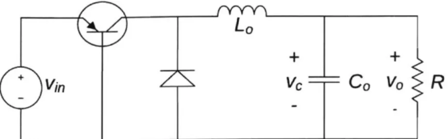
In this section, the PI controller parameters of DC-DC Buck converter, as shown in Fig.1 [24], is determined by the proposed game theory based method. Other types of DC-DC converters can also apply the proposed method to get optimal controller parameters. The input voltage of the Buck converter is 36 V initially and drops to 24 V at 0.015s, and the output voltage is expected to be maintained at 15V.

VC CO vo R

Figure 1. Circuit schematic of a buck converter. The state space model of the Buck converter above is

di q(t)v, (t) ₍₃₉₎

dt Lo Lo

dv, _ t(t) v" (40)

dt Co CORo

where q(t) is 1 when switch is on and 0 when off. Then following transfer function can be derived for the corresponding averaged model:

H(= D (s) (s2LoCo+s +1)

(41)

where D is the duration for switch is on. Assume the input to Hi(s) is I/s, a step response, which means a sudden change in the input voltage, the error of output voltage in frequency domain can be expressed as

e(s) = H(s)(43)

s[1 - _{(K, + K,)H}

2(s)]

To make the system stable, K, and Kp should be picked up within the range of (44) below.

K,, <-, K, <0 (44)

_J'Y-Y-Y-'

-- I I-- Lo

Applying the method described in 1II, ITSE and ISTSE expressions made up by K and Kp can be generated. After 6 iterations of gaming, the tuning parameters can be determined to be Kp = -0.0 16 and Ki= -93.

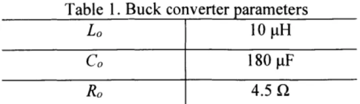
Fig.2 plots the output voltage responses of the system in Fig.4 by using the proposed game theory based tuning method, compared with MATLAB Simulink optimal tuning function (which is based on minimum integral of time-weighted error) and traditional Ziegler-Nichols tuning method, when input voltage drops to 24 V from 36 at 0.015s. The parameters of the circuit can be seen in Table 1. As can be seen from Fig.2, by using the game theory based controller tuning method, the output voltage recovers much faster after the input voltage drops than using the MATLAB Simulink optimal tuning function and the traditional Ziegler-Nichols tuning method. Besides, the maximum output voltage drop is also the

smallest among three tuning methods.

15 14 :913 012 _{- Game Tuning} -- Matlab Tuning 11 . - ziegler-nichols 0.016 0.018 0.02 0.022 Time (s)

Figure 2. Comparison of game theory based tuning method with MATLAB optimal tuning and ziegler-nichols method.

Table 1. Buck converter parameters

Lo 10p H

Co 180pF

Ro 4.5 Q

In order to plot the Pareto Frontier of the multi-objective optimization model (6) of the DC-DC controller tuning problem, 6000 random combinations of Ki and Kp within the nominal stability range are generated by sweep over the two dimensional space to get 6000 values of corresponding ISTE and ISTSE. For better visualization, all the data are normalized such that minimum ISTSE happens at normalized ISTE equals 1 and minimum ISTE happens at normalized ISTSE equals 1. Only the points that can form Pareto Front are kept and are plotted in Fig.3, along with the Nash Equilibrium point generated from the proposed game theory based tuning method.

As can be seen in Fig.3, for the DC-DC buck converter controller tuning problem, the Nash Equilibrium locates at the Pareto front of the corresponding Multi-objective optimization. For other Multi-objective optimization problems with conflicting objectives and more variables, the Nash Equilibrium point might not be located on the corresponding Pareto front. In those cases, the final solution can be chosen from the Pareto front by finding the solution that is closest to the Nash Equilibrium. By doing this, the Nash Equilibrium is treated as a reference to help the selection of final solution, in which case, both global and individual optimal is considered.

0.9 0.8 0.7 0.6 0.5 0.4 0.3 0 0.2 0.4 0.6 0.8 1 Normalized IS TE

Figure 3. Plot of the Pareto Front and Nash Equilibrium point.

U.' I,

3. Cooperative Game Theory Based Local

Power Exchange Algorithm for Networked

Microgrids

3.1. Background

In a traditional power system, loads are serviced by the distribution grid: The required power is delivered from the main grid through transmission lines. The addition of microgrids helps relieve the burden on the main grid and improves reliability in certain areas. Even though large-scale renewable energy can be integrated into electric power systems, the intermittent nature of wind and solar power poses new challenges to the operation and control of autonomous microgrids, especially with high penetration levels [25].

Another challenge is that the relatively small power scale of microgrids makes it difficult to accurately forecast future net power output. These two problems mean that at times microgrids will need extra power from the main grid in grid-connected mode and establish a need for certain reserves on the main grid side to guarantee reliability. To address these problems, researchers have proposed many ideas to improve reliability of operation and achieve more accurate renewable energy and load forecasting for microgrids in traditional operation situations

[26]-[32].

Given the fact that future distribution networks may encompass a large number of local microgrids, instead of trying to solve the above mentioned problems from the perspective of a single microgrid in traditional operation situations, authors in

[33] and [34] proposed cooperative game-based networked microgrid local power

flow exchange scheduling, which facilitates microgrids' cooperation from a new perspective. It is beneficial for the microgrids with a power deficit to exchange

power locally with microgrids with an excess of power, instead of getting the power from the main electricity grid [33].

The advantages of such a local exchange for line losses and reserve saving are fourfold: 1) Because the distance between neighboring microgrids is usually much shorter than between microgrids and the specific transmission substation, line losses for local power exchange between microgrids are usually much smaller. 2) Power losses on main grid transmission lines are also reduced because cooperating microgrids need less power from the main grid. 3) Power losses at the transmission substation transformer level can be reduced. Finally, 4) cooperative microgrids can behave as an entity, thus increasing the power scale and achieving larger geographical coverage, which in turn helps improve the forecasting accuracy of integrated renewable energy and the serviced load of those microgrids. As a result, the reserve needed from the main grid to ensure reliability can be reduced, which can in turn reduce costs. Given these benefits, an algorithm that can model and promote local power exchanges between buyer microgrids (those in need of power) and seller microgrids (those with surplus power) is worth studying.

Based on [34], more and more researchers have proposed algorithms using cooperative games to model cooperative power exchange mechanisms for this local power exchange [35]-[42]. However, there are two principal problems with those proposed mechanisms. The first is that geographically closer microgrids are usually designed to exchange power first. But in many real cases, this may not yield optimal utility, since trading with more distant microgrids may save even more power, thus increasing utility.

In addition, different seller microgrid and buyer microgrid trading pairs will, in real life, have different trading prices. In other words, an energy exchange between a seller microgrid group and a buyer microgrid group should be modeled using game theory rather than an optimization scenario that assumes the same price for all trading, because all the units in those local microgrids are owned by

different entities. Since every entity pursues maximum utility, optimization may result in lower utility for some entities, which would then lose their incentive for cooperation.

Three sub-problems need to be addressed in designing such a cooperative game-based local power exchange algorithm for networked microgrids. The first is to match seller microgrids and buyer microgrids in every possible coalition so as to achieve maximum coalition utility. After the coalition's total utility is calculated, a fair utility allocation should be made according to each microgrid's contribution. And finally, an optimal coalition partition among all possible coalition combinations must be chosen.

This chapter proposes a cooperative game-theory-based local power exchange algorithm for networked microgrids, created in three steps: 1) An auction-theory-based matching method is proposed for calculating the maximum utility of every possible coalition. 2) The Shapley value method is applied to fairly distribute the utility of every coalition among its members. 3) Coalition merging and splitting techniques are introduced to find the optimal partition among all possible coalition combinations.

The rest of this chapter is organized as follows. Section 3.2 describes the structure of networked microgrids and the traditional non-cooperative operation situation. Section 3.3 introduces the auction-theory-based method for calculating the utility of every valid coalition. Section 3.4 focuses on the Shapley value method for distributing total coalition utility among its members and the method for selecting the optimal partition of coalitions. The results of the simulation test are presented in section 3.5.

3.2. Networked microgrids Model

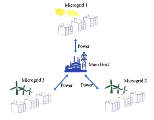
This section explains the structure of networked microgrids and traditional non-cooperative operations. Consider the scenario of a distribution network in which

N microgrids are connected to a transmission substation that is connected to the

main power sources (e.g., solar farms and wind farms) in different power scales, as shown in Fig. 4 below.

Microgrid 1 Power

4a

Figure 4. Traditional microgrid system.

In any given period of time, every microgrid in the local network can generate a certain amount of power by its micro-sources and needs a certain amount of power to meet its demand side power consumption. If the net output power of a microgrid is greater than zero, the microgrid is defined as a seller microgrid with e; > 0. Similarly, if its net output power is less than zero, the microgrid is defined as a buyer microgrid with di < 0. Traditionally, unbalanced power in microgrids is

evened out by the main grid in grid-connected mode, given the fact that not enough energy storage is available [43]. In other words, seller microgrids will sell their excess power to the main grid through a transmission substation, and buyer microgrids will buy the needed power from the main grid, also through the transmission substation. In this traditional non-cooperative and individual

for seller and buyer microgrids, respectively [44]: e 2 R ),L = 2" + fpe (45) 0 J s R,₀ O2S = (46)

where Pios is the power supplied from the transmission substation so that buyer microgrid b, can get the power required to fulfill di. This can be solved with the equation below:

p2R

S=" + P S -d, (47)

0

For a power exchange between microgrids to fulfill the power requirement of di, the losses can be calculated as shown in (48) and (49):

P2 R

Ys- d, (48)

L - 'j- s R, (49)

From the formulas above, it can be inferred that networked microgrids have an incentive to cooperate in local power exchanges with neighboring microgrids. This is because in a local power exchange, , will be zero, as there is no loss in the transformer in the transmission substation, and the transmission distance is shorter.

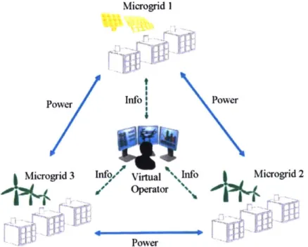
When microgrids in a network choose to cooperate in order to get higher individual utility, they can coordinate their strategies to behave as a coalition

-as if there is a network virtual operator where they can share current power state information, as in Fig. 5. A cooperative game with transferable utility can be defined as (N, v), where the utility function v(S) describes how much total utility the coalition S can achieve if some players in N decide to cooperate and form coalition S. To calculate the individual utility and facilitate this cooperation, a three-step algorithm needs to be executed for the virtual network operator: 1)

calculated coalition utility among coalition members. And 3), according to the utility allocation, determine the optimal coalition partition for the network. These

steps will be explained in the following sections. Microgrid 1

Power

Microgrid 3 In

~zizp

Info Power

foo/ Virtual Info Microgrid 2

Operator \

Power

Figure 5. Illustration of networked microgrids system with virtual operator.

3.3. Coalition Utility Calculation

This section introduces the auction-theory-based coalition utility calculation method: Given any valid coalition S that says there is at least one buyer microgrid and one seller microgrid in S, divide the coalition members into buyer microgrid group Gb and seller microgrid group G. In any period of time, any microgrid bi E Gb is in need of power and is willing to buy power from another source. Similarly,

any microgrid q; E G, has excess power to sell. Given the fact that each different power trading pair {bi, qj} has a different trading cost depending on distance, for every possible coalition a fair and efficient method is needed to match the members in Gs and Gb so as to achieve efficient local power exchange with high coalition utility.

The matching problem was first introduced by Gale and Shapley [45] in 1962. After them, different matching models have been proposed and applied in many areas, such as biological computation [46], pattern recognition [47], operation research [48], and computer vision [49]. However, to authors' knowledge, none of the famous existing matching models [50]-[53] are suitable for this networked microgrid cooperative local power exchange situation. The reasons are twofold: 1) Most existing models assume the traded goods are indivisible, which is not the case for electric power, and 2) as shown in formulas (1)-(3), there would be power losses in the process of trading that depend on the amount of traded power, thus the unit price of electric power will change for each different traded quantity. Actually, power trading among those microgrids in the situation described is quite different from the power market of the transmission grid. In the transmission grid, line loss is not a key factor when calculating the clearing price in the market pool after power sellers and buyers submit their bids [54]. However, for networked microgrids at the distribution level, line loss should be considered for cost calculation as line impedance is higher.

The typical matching method for this local power exchange setting is proposed in [33]: For every possible order of the buyer microgrids in Gb in any given valid coalition, starting from the first buyer microgrid, the method ranks seller microgrids in Gs based on the distance to the buyer microgrid, and trades according to this order. If any buyer microgrid (or seller microgrid) buys (or sells) all of its demand (or excess), it will be deleted from Gb (or Gs) and the next one in

line will have the opportunity to trade, in order, based on the new distance. Every trade in this method is designed to have the same unit power price. The buyer order and corresponding trading process that can yield maximum coalition utility will be selected. Other cooperative operation methods mentioned in Section II also assume the rules that the closest buyer and seller microgrids should trade first, and the trading price should be the same within the network.

microgrids farther from other microgrids usually will not have opportunity to trade. This may not be the case in reality, as those buyer (or seller) microgrids far from other seller (or buyer) microgrids may prefer to pay more as compared with closer buyer (or seller) microgrids in order to avoid trading with the main grid through a transmission substation, simply because trading with the main grid might generate higher costs. Closer microgrids might not lose too much utility while trading with the main grid. It is also unrealistic to assume that every microgrid in the network will have the same unit price for trading power, as all the units in those local microgrids in the network are owned by different entities, and every entity pursues maximum utility. Thus game theory is more suitable for this multi-agent problem than optimization.

Another problem with these existing algorithms is that in any coalition, buyer

(or seller) microgrids are restricted to avoid trading with the main grid until no seller (or buyer) microgrids are available. This may not be a good way to

calculate coalition utility, because in some cases, trading with the main grid can save more losses if the microgrid is close enough. Considering all these facts, a second-price sealed bid auction-based algorithm for matching seller microgrids and buyer microgrids in a given coalition is proposed below. The trading pairs will be determined according to the bids that members in Gb are willing to provide to members in Gs.

Assume there are m microgrids in Gb and n microgrids in G, in a coalition, and

Gb {bi, b2,..., bm} has demanded power D = {dl, d2,..., dm,} and Gs {qi, q2,..., qn} has excess power E = {ej, e2,..., en} to sell. Given any seller microgrid q and

buyer microgrid bi, the corresponding power Pij.s supplied from qj so that bi can

receive di to meet its power requirement can be calculated according to (48) above. The maximum amount of power P,, s, that qj can supply to bi is min{Pijs, ej1}.

Substituting Py, smax in equation (49), the maximum received power Pij, ma for bi

corresponding P1, Rp can be calculated as shown in (50) below.

hi = '% go's'ax i sax (50)

In general, for any qj, every bi can have a price-quantity bid {hi, PY. smax}. Similarly, the lowest price l0 that qj is willing to accept from b, is calculated as

follows:

o, =oj,R cog /e₁ (51)

In this case, the transmission substation acts as a buyer microgrid with the price-quantity bid {loj, ej}. Then Gb = {b1, b2,..., b, substation} with

corresponding demanded power D = {dj, d2,..., d, e1} and bid prices H = {hi,

h2,..., hm, loj}.

Define ly as the income per unit power if PU1 smax is traded between seller

microgrid qj and a transmission substation instead of with buyer microgrid bi. It is calculated as follows:

l = P, -nax 'g / Pisnax (52)

In order to get trading pairs within the members of Gb and Gs, a many-to-many

matching situation is simplified to this many-to-one second-price sealed-bid auction scenario, given Gb and a seller microgrid qi from Gs. In this scenario, the

buyer microgrid with the highest bid price hs,5 will have the opportunity to trade qi

at the second highest bid price h2nd if there are at least two bid prices higher than the corresponding lowest acceptable price loj. If only one buyer has a bid higher than the lowest acceptable price, the clearing price would be the average of them. When lj is the highest bid, no trading occurs between microgrids, because the

seller microgrid will sell all its excess power to the transmission substation [55],

[56]. It is proven that every bidder in this second-price sealed-bid auction

situation has the incentive to submit a real price-quantity bid [57]. Given the random order of the members in Gs, the many-to-one auction will be repeated according to the order until no sellers or buyers are available to trade or no bid is higher than lj. Then the coalition utility for this given order of the members in Gs

can be calculated as shown in (53) below, which sums up all the coalition incremental utility in every trading pair for trading the same amount of power, from non-cooperative to cooperative situations.

v(S) =(- (lPs -C ij (ljSniar Wg to,Smax)(3P0 s (53)

leGh,EG,

Every possible member order in Gs will be tried and the corresponding utility calculated. The order that can generate the maximum coalition utility will be selected as the final order for Gs and the corresponding utility will be treated as the coalition utility. By applying this repeated second-price sealed-bid auction rather than the double auction methods in the traditional many-to-many matching problem, trading pairs between buyer and seller microgrids can be determined, and all the generated coalition utility values for different member orders in G, will be used in calculating utility allocation by Shapley value (covered in the next section). Table 2 below gives a detailed procedure for this coalition utility calculation method, to be executed by the virtual operator.

Table 2. Auction Based Coalition Utility Calculation Algorithm

repeat

Given a random member order in Gs for coalition S.

repeat

(a) Denote the first member in current Gs as qj.

(b) Calculate the price-quantity bid (hi, Py,s1 ax) for every member in Gb and

lowest acceptable price 101 and li

case 1: At least two buyer microgrids have a bid price higher than l. Then

bis trades with qj at h2nd. if Pq.sax = ej

Gs = Gs\ qj, E = E \ ej and dis ₁= dis, - Py,Rmax else

Gb = Gb \ bis,, D = D \ dist and ej = ej -Pj.smax

with qj at (hist -loj)/2. if Pi.smax = ej

Gs = Gs \ qj, E = E \ e, and dis, = dis, -Pj,Rmax

else

Gb = G\ bis, D = D \ dis, and ej = ej - P4,smax

case 3: No buyer microgrids have a bid price higher than lo for qj, Gs = Gs \

qj.

until Gs or Gb is empty or no more trades can be made, calculate the coalition

utility by (9)

until all possible member orders in Gs have been tried output the member order in G, with max coalition utility

3.4. Coalition Utility Allocation and Optimal Coalition Structure

In this section, we will first apply the Shapley value method to distribute the coalition utility generated in section 3.3 for all valid coalitions. In the second part, a method for selecting optimal partition among all possible coalition combinations will be introduced.

3.4.1. Coalition Utility Allocation Based on Shapley Value

After the coalition utility is calculated, a way to distribute the utility among its members is needed. Shapley value is a useful solution in cooperative game theory because it emphasizes fairness. For each cooperative game, the Shapley value allocates the total utility generated by the coalition among the members of the coalition based on each member's contribution to the total. The payoff of every member is calculated when it is the first to enter the game, the second, and the third. The average value of coalition incremental payoffs in every permutation order determines the payoff to each member [58]. Therefore, influence from entry order is eliminated in calculating the individual payoff. The Shapley Value is characterized by a collection of desirable properties as follows.

Axiom 1 (Efficiency): Total utility is distributed:

E = v(S) (54)

kES

Axiom 2 (Symmetry): If {i} and {j} are two members that are equivalent such

that

v(S u{i})= v(S u{j}) (55)

for every S which contains neither {i} nor

{/},

= (56)

Axiom 3 (Linearity): If two coalitions with utilities u and w are combined,

then

"k=(P"+" (Pk(57)

Axiom 4 (Null Player): Player {k} is null if for every coalition it makes no

contribution:

v(Su{k})= v(S) (58)

The distributed utility for the null player is zero.

Given a coalition S, it is proven that the Shapley value, as calculated below in (59), is the only map from the set of all games to payoff vectors that satisfies all four axioms above [59].

Sbk k= SI [v(S u{k})-v(S,)] (59)

Note that in this networked-microgrids cooperative game, utility is divided among the members in any formed coalition S, and a merge and split technique will be used later to find a stable coalition partition in the network. Therefore, equation (59), which is usually used to find the utility division for the grand coalition by Shapley value, would be used on every valid coalition S in the game.

3.4.2. Optimal Coalition Partition of Network

After utility and the corresponding allocation are calculated for every possible valid coalition, given any initial partition of the network, some microgrids may

want to join other coalitions for greater individual utility; in other words, the current network partition is not stable. A method is needed to find the stable coalition partition of the network among all possible coalition combinations, and using Pareto order as this method is defined in [33] and [60].

Definition 1: Given two collections of disjoint coalitions R {ri,..., r} and Z

= {zj, ... , zn} formed from the same players in a grand coalition, collection R is

preferred over Z by Pareto order if and only if

R > Z c {f~ > (pVk e R, Z} (60)

with at least one strict inequality (>) for a player k.

According to the definition of Pareto order, a group of microgrids in the cooperative game prefers to become part of collection R instead of Z if at least one member is able to improve its individual utility, without sacrificing the utility of any other members, if the partition of the network is changed from Z to R. Then the following two rules of merging and splitting for coalition formation can be applied to find the stable partition of the network [60].

Definition 2 (Merging Rule): Merge any set of coalitions {S,,...,S,} where

{u'I S} c> {S,..S,} ; therefore, {S1,...,S,} - {u'jS}

Definition 3 (Splitting Rule): Split any set of coalitions u', S, where

{S₁,..., SI} > {u's S1 } ; therefore, {=' Sj,,} -+ S

The merging process can help small microgrid coalitions form bigger coalitions if greater utility can be achieved for some microgrids among them and no microgrids are sacrificed. Similarly, the splitting process can also help large coalitions divide into small coalitions if no microgrids are sacrificing their utility after the splitting process, and some microgrids achieve higher individual utility. Iteratively applying the rules of merging and splitting, Dc-stable state, which is defined as a state in which no players have incentives to leave their current coalition and form a new partition for the network, can be achieved given any

3.5. Simulation Results and Analysis

In this simulation, the proposed cooperative game-theory-based algorithm is first compared with the traditional non-cooperative operation situation to show individual utility improvement and loss reduction. In the second and third part of this simulation, performance and efficiency of the proposed algorithm, respectively, will be shown.

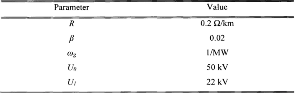
Throughout this simulation, microgrids are randomly generated in an area of 12 km x 12 km with the transmission substation located at the center of the area. Corresponding selected parameter selection can be found in Table 3.

Table 3. Parameter selection for simulation

Parameter Value R 0.2 Q/km p8 0.02 WOg 1/MW UO 50 kV U 22 kV

In order to emphasize the utility improvement, all microgrids are assumed to have lines connected with other microgrids in the network. The proposed algorithm will be applied in this setting to find out how the microgrids will operate cooperatively so as to improve their individual utility. In reality, it is unrealistic to have connection lines between all microgrids in a local area. In these cases, the proposed algorithm can be applied to the connected local microgrids, or can be used to provide line construction suggestions for unconnected local microgrids, if there are potential coalitions that can make enough profit if all lines are connected.

3.5.1. Example of 13-Microgrid Network

Fig. 6 below shows a local distribution network with 13 randomly generated microgrids. There are, in total, four seller microgrids and nine buyer microgrids. Given any period of time, every microgrid in the network has a certain amount of power to sell or to buy randomly, in the range of 0 MW to 100 MW. After the proposed algorithm is applied, a total of four coalitions are finalized, shown by the red dashed circles. In this scenario, no microgrid wants to leave its current coalition and join another coalition. In coalition I, seller microgrid 11 will first meet the extra power requirements of buyer microgrids 12 and 10 and then meet part of the power requirement of buyer microgrid 7, which later buys the remaining 10 MW required power from the transmission substation. Note that

seller microgrid 11 will trade with buyer microgrid 12 first, even though buyer

microgrid 12 is approximately the same distance from microgrid 11 as from microgrid 10 and is farther from the transmission substation. Similarly, in coalitions III and IV, seller microgrid 4 will fulfill the need of buyer microgrids

13 and 9 first, and then provide part of the power requirement of buyer microgrid

5. Seller microgrid 6 will fulfill the need of buyer microgrids 8 and 3 first, then

sell its remaining excess power to the transmission substation. Note that even though microgrid 9 has the longest distance to the transmission substation, it will still trade with microgrid 4 before microgrid 5, because it has a higher bid and can thus create more coalition utility. Similarly, microgrid 8 will trade with microgrid

Coalition I J MG + -'33 MW 9% to MG 12 5 76% tD MG 10 1 15% to MG 1 MG 12 4MW4 100% frof MG 11 6 4 2 0 -2 -4 -2 10 MW \ from MG 11' Sb 0 Position X (Km) -G 1 MW from MG 4 MG 4 42 MW 57% to 13 38% to MT 9 5% to Mq5 MG 9 -16 MW 00% from MG 4 MG 5 jMW 29%rom PG 4 71% frdms bstation Coalition III (camftion IV, MG 6 MG 3 20%to MG 8 100% from G 64 3 % tO su J -1 MW 100% fron"lG 6 2 4 6

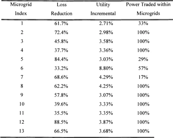
Figure 6. Stable coalitions of the 13-microgrid network.

As shown in Table 4 below, in this local distribution network with 13 randomly generated microgrids, nine microgrids sell or buy all their excess or required power with other microgrids instead of with the transmission substation. For power traded between microgrids instead of with the transmission substation, individual incremental utility and loss reduction are also shown in the table. On average, there is a 3.87% individual utility increment and 52.87% line loss reduction. Mp I -15 MW 33% from MG 11 #7 frtm sub-saton MG 7 -48 MW 17% from MG 2 83% from sub-stat4 MG 2 BMW -4 Caio 1b1,~ 0 0L -4 -6 '--6 I I