Applications of time series analysis to geophysical data

APPLICATIONS OF TIME SERIES ANALYSIS to

GEOPHYSICAL DATA

by

ALAN DANA CHAVE

B. S., Harvey Mudd College (1975)

SUBMITTED IN PARTIAL FULFILLMENT OF THE REQUIREMENTS FOR THE

DEGREE OF

DOCTOR OF PHILOSOPHY

at the

MASSACHUSETTS INSTITUTE OF TECHNOLOGY and the

WOODS HOLE OCEANOGRAPHIC INSTITUTION June, 1980

Signature of Author

-Joint Program in Oceanography, Massachusetts Institute of Technology-Woods Hole Oceanographic Institution, and the Department of Earth and Planetary Sciences, Massachusetts Institute of Tchnology, May, 1980,

Certified by___

Thesis Co-supervisor Certified by

Thesis Co-supervisor Accepted by

Chairman, Joint Oceanography Committee in the Earth Sciences, Massachusetts Institute of Technology-Woods Hole Oceanographic Institution

MASSACHUSE _jO]1, OF TECHNOL _1

MjTl

RIES

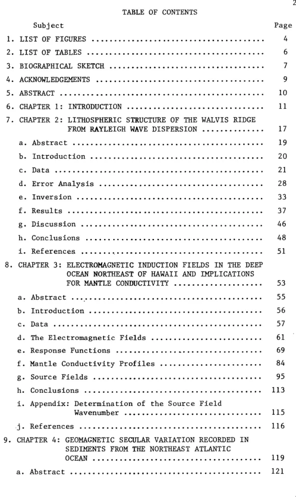
TABLE OF CONTENTS Subject LIST OF FIGURES .... LIST OF TABLES BIOGRAPHICAL SKETCH ... ACKNOWLEDGEMENTS ... ABSTRACT ... ... CHAPTER 1: INTRODUCTION ... CHAPTER 2: LITHOSPHERIC STRUCTURE OF THE WALVIS RIDGE

FROM RAYLEIGH WAVE DISPERSION ... a. Abstract ... b. Introduction ... c. Data ... d. Error Analysis ... e. Inversion ... f. Results ... g. Discussion ... h. Conclusions ... i. References ...

8. CHAPTER 3: ELECTROMAGNETIC INDUCTION FIELDS IN THE DEEP

OCEAN NORTHEAST OF HAWAII AND IMPLICATIONS FOR MANTLE CONDUCTIVITY ... a. Abstract ... b. Introduction ... c. Data ... d. The Electromagnetic Fields ... e. Response Functions ... f. Mantle Conductivity Profiles ... g. Source Fields ... h. Conclusions ...

i. Appendix: Determination of the Source Field

Wavenumber ...

j. References .. ...

9. CHAPTER 4: GEOMAGNETIC SECULAR VARIATION RECORDED IN SEDIMENTS FROM THE NORTHEAST ATLANTIC

OCEAN ... a. Abstract ... .... . . ... . ... . ... ... .. ... Page 4 6 7 9 10 11 17 19 20 21 28 33 37 46 48 51 53 55 56 57 61 69 84 95 113 115 116 119 121

3

b. Introduction...122

c. Regional Sedimentary Environment ... 123

d. Stratigraphy ... 126

e. Paleomagnetic Data ... 141

f. Spectral Analysis ... 156

g. Discussion ... 165

h. Conclusions ... 174

i. Appendix: Quantitative Assessment of Stratigraphic Correlation ... 175

LIST OF FIGURES

Page CHAPTER 2

1. Location map showing the surface wave paths to stations

SDB and WIN ... 22

2. Airy phases for the two events at SDB and WIN ... 26

3. Group velocity dispersion curves for the on-ridge and off-ridge paths ... 30

4. Partial derivatives of group velocity at three periods for the final ridge model ... ... 35

5. Shear velocity structure from inversion of the dispersion curves for the on-ridge and off-ridge paths ... 38

6. Group velocity residuals from both inversions ... 41

7. Resolving kernels for the velocity models ... 43

CHAPTER 3 1. Location map for electromagnetic instrumentation ... 58

2. Time series for the electric and magnetic field data .. 62

3. Separation of 5 tidal lines from the east magnetic field component ... ... 67

4. Smoothed power spectrum for the electric field data ... 70

5. Smoothed power spectrum for the magnetic field data ... 72

6. Composite signal to noise variance ratio as a function of the data matrix rank ... 77

7. Signal to noise variance ratio by data component for a rank 2 signal matrix ... ... 80

8. Signal to noise variance ratio by data component for a rank 3 signal matrix ... 82

9. Response functions from the SVD and least squares a analyses ... . ... ... 85

10. Conductivity structure from inversion of the response functions ... 92

11. Conductivity structure of this study compared to other results ... 96

12. Tipper coherence ... 99

13. Tipper function ... 101

14. Polarization diagrams for quiet time variations ... 106

15. Polarization diagrams for storm time variations ... 108

16. Model response curves for induction by moving source fields ... .. ... ... 111

CHAPTER 4

1. Index map showing physiography of the North Atlantic

Ocean and the detailed study area ... 124

2. Sediment isopachs and bathymetry for detailed study area ... 127

3. Raw stratigraphy for five piston cores ... 132

4. Signal and residual EOF's for two and three age picks . 137 5. Stratigraphy plotted against age for five cores ... 139

6. Age against depth for five cores ... 142

7. Pilot sample demagnetization curves ... 146

8. pNRM/pARM behavior of a typical pilot sample ... 149

9. Paleomagnetic time series of directions ... 152

10. Paleomagnetic time series of relative paleointensities 154 11. Normalized length criteria for PEF calculation ... 160

12. Unit circle distance for PEF length calculation ... 162

13. Maximum entropy power spectra of complex equivalent directions ... ... ... 167

LIST OF TABLES

Page

CHAPTER 2

1. Epicenter information ... 2. Group velocity data ...

3. Final model parameters ... CHAPTER 3

1. Tidal amplitudes and phases ... 2a. SVD response functions ... b. ZB response functions ...

E

c. Z response functions ... 3. Electrical conductivity structure ... CHAPTER 4

1. Planktonic foraminiferal assemblages .. 2. Chronostratigraphic horizons ... 3. Pilot sample data ...

4. Principal spectral bands ...

66 87 88 89 94 131 135 145 166 ... ... ... . . . .. .. . . O0 0 0... 0 0 00

BIOGRAPHICAL SKETCH

I was born in Whittier, California on 12 May 1953. I attended Harvey Mudd College, Claremont, California from 1971 to 1975 and was graduated in June, 1975 with a Bachelor of Science degree in physics, awarded with distinction and departmental honors. My introduction to oceanography came during the summers of 1972-1974, when I worked for the late Dr. Wilton Hardy at the University of Hawaii. In June, 1975, I enrolld in the Woods Hole Oceanographic Institution-Massachusetts Institute of Technology Joint Program in Oceanography. My work has

covered portions of the fields of earthquake seismology, magnetotellurics, and paleomagnetism with an emphasis on quantitative analysis of

geophysical data. After participating in Leg 74 of the Deep Sea Drilling Project, I will be a postdoctoral investigator in the Geological Research Division of the Scripps Institution of Oceanography.

My publications include:

1. Chave, A.D., R.P. Von Herzen, K.A. Poehls, T.H. Daniel, and C.S. Cox, 1978. Deep ocean magnetotelluric sounding in the northeast Pacific, EOS 59, 269 (abstract).

2. Chave, A.D., 1978.Lithospheric structure of the Walvis Ridge from Rayleigh wave dispersion, EOS 59, 1199 (abstract).

3. Chave, A.D., J.D. Phillips, and D.W. McCowan, 1978. Lithospheric structure of the Walvis Ridge from Rayleigh wave dispersion,

Semi-annual Technical Summary, Lincoln Laboratories Report 78-259, pp. 49-50.

4. Chave, A.D. and C.R. Denham, 1979. Climatic change, magnetic intensity variations,and fluctuations of the eccentricity of the earth's

orbit during the past 2,000,000 years and a mechanism which may be responsible for the relationship--a discussion, Earth Pl. Sci. Lett. 44, 150-152.

5. Chave, A.D. and R.P. Von Herzen, 1979. Electrical conductivity structure at a deep ocean site northeast of Hawaii, EOS 60, 243

(abstract).

Electrical conductivity structure at a deep ocean site northeast of Hawaii, in Proceedings of Workshop on Ocean Floor

Electromagnetics, Naval Postgraduate School, Monterey Ca., 20-22 August 1979 (abstract)

7. Chave, A.D., 1979. Lithospheric structure of the Walvis Ridge from Rayleigh wave dispersion, J. geophys. Res. 84, 6840-6848.

8. Chave, A.D., G.P. Lohmann, and C.R. Denham, 1979. Quantitative

evaluation of biostratigraphic correlation, EOS 60, 854 (abstract). 9. Denham, C.R. and A.D. Chave, 1979. Late Pleistocene paleosecular

variation in marine sediments from the Gardar Drift, NE Atlantic Ocean, EOS 60, 818 (abstract).

10. Chave, A.D., R.P. Von Herzen, K.A. Poehls, and C.S. Cox, 1980. Electromagnetic induction fields in the deep ocean northeast of Hawaii and implications for mantle conductivity, submitted to Geophys. J. Roy. astr. Soc.

11. Chave, A.D. and C.R. Denham, 1980. Geomagnetic secular variation recorded in sediments from the northeast Atlantic Ocean,

ACKNOWLEDGEMENTS

The three papers that comprise this thesis represent the products of interaction with many people. I would particularly like to

acknowledge the support and encouragement of Dick Von Herzen, whose example as a scientist will always mean a great deal to me. Among the other people at Woods Hole, Chuck Denham and Pat Lohmann provided many useful discussions on data analysis and other topics.

The Walvis Ridge study was originally suggested by Tom Crough while he was a postdoctoral scholar at WHOI. Joe Phillips and Doug McCowan of the Applied Seismology Group at MIT's Lincoln Laboratory gave me access to their computer facilities and programs for surface wave inversion.

The magnetotellurics study is the result of a multi-institutional program with Scripps and the University of Hawaii. Tom Daniel (U. of Hawaii), Jean Filloux (Scripps), and Ken Poehls (UCLA) were present on

the instrument deployment cruise. Chip Cox (Scripps) provided the electric field data for this study. Jack Hermance (Brown University) and Jim Larsen (PMEL, Seattle) improved my understanding of induction processes immensely.

The paleomagnetic study is the result of a great deal of work with Chuck Denham and Pat Lohmann. Bill Ruddiman (Lamont) gave me a

great deal of useful information on North Atlantic stratigraphy. Most of the results of this thesis would not be possible without the breakthrough in computing power represented by the VAX line made by the Digital Computer Corporation. Finally, I would like to thank

the breweries of the world whose product contributed materially to many discussions.

I was supported for the early parts of this work by a NSF Graduate Fellowship. The Walvis Ridge study was supported by the WHOI Education Office and the Defense Advanced Research Projects Agency. The induction study was funded by the NSF under grants

0CE74-12730 and 0CE77-8633, and by the WHOI Ocean Industries Program. The paleomagnetic study was supported by NSF contracts 0CE77-82255 and 0CE79-19258.

THE APPLICATION OF TIME SERIES ANALYSIS to

GEOPHYSICAL DATA by

Alan Dana Chave

Submitted to the Woods Hole Oceanographic Institution-Massachusetts Institute of Technology Joint Program in Oceanography on May 2, 1980 in partial fulfillment of the requirements for the degree of Doctor of Philosophy.

ABSTRACT

This thesis consists of three papers applying the techniques of time series analysis to geophysical data. Surface wave dispersion along the Walvis Ridge, South Atlantic Ocean, is obtained by bandpass filtering the recorded seismogram in the frequency domain. The group velocity is anomalously low in the period range of 15-50 s, and formal inversion of the data indicates both crustal thickening to 12.5 km and low shear velocity (4.25-4.35 km/s) to depths of 40-50 km. The electromagnetic induction fields at a deep ocean site northeast of Hawaii were used to determine the electrical conductivity of the earth

to 400 km depth. Singular value decomposition of the data matrix

indicates three degrees of freedom, suggesting source field complications and a two dimensional conductive structure. Inversion of one of the principal terms in the response function shows an abrupt rise in

electrical conductivity to 0.05 mho/m near 160 km with no resolvable decrease below this. A model study suggests that moving source fields

influence the induction appreciably in the other principal response function. A set of piston cores from the northeast Atlantic Ocean are used to construct paleomagnetic time series covering the interval

25-127 kybp. Stratigraphic control is provided by counts of planktonic foraminifera, and empirical orthogonal function analysis shows a

significant decrease in sedimentation rate at the interglacial/glacial

transition. The sediments are magnetically stable and reliable relative

paleointensity measurements could be obtained. Spectral analysis of

the directions reveals a predominant 10 ky periodicity and no dominant

looping direction.

Thesis Co-supervisor: Charles R. Denham Title: Associate Scientist

Thesis Co-supervisor: Richard P. Von Herzen Title: Senior Scientist

11

CHAPTER ONE

The quantitative treatment of sequences of data constitutes the field of time series analysis. A single data variable or a field of variables, measured as a function of a well determined dependent

quantity like time, is a time series or sequence. The techniques of time series analysis are commonly used in disciplines from economics and engineering to oceanography and geophysics as a means of extracting information from long, complex data sets. Applications include

the detection of hidden periodicities, the analysis of variance or power, and the quantitative estimation of statistical correlation.

Time series analysis has been an important tool of the geophysicist since the advent of the physical study of the earth. Early

seismologists were limited by the lack of computing machines and developed manual techniques to analyze time series. The first applications to seismograms were limited to the picking of arrival times and amplitudes. The analysis of periodic data, especially earth tides, was also accomplished by hand fitting. Much of this early work is described by Jeffreys (1959) and Bullen (1963).

The introduction of inexpensive and efficient digital computers has resulted in increasingly more elegant and complex analyses of

time series. Extensive use is made of the Fourier transform, especially since the rediscovery of the fast Fourier transform algorithm. The equivalence of the time-space and frequency-wavenumber domains is well established. Theoretical expressions in geophysics are often more easily derived in the frequency domain, and it is not uncommon to examine only the frequency domain behavior of a data set. Other geophysical techniques, notably interpolation, least squares fitting, and inverse problems, have been applied to data as computer technology has improved. Bath (1974), Kanasewich (1975), and Claerbout (1976) discuss many uses of these methods,, with an emphasis on seismology. The techniques are also employed in the modelling of marine magnetic anomalies (Schouten and McCamy, 1972) and in the analysis of gravity lines (McKenzie and Bowin, 1976; Detrick, 1978).

Theoretical advances in time series analysis have followed a parallel course to its applications. Much of the early work in the field is based on classical statistics, especially the auto and

as the Fourier transform of the autocorrelation function. Many computational problems exist with this approach due to inherent and incorrect assumptions about long term time series behavior.

Additional treatment of the correlation function is necessary to

minimise bias and leakage (Blackman and Tukey, 1958; Jenkins and Watts, 1968). The increasing use of the discrete Fourier transform

minimized some of these problems and introduced some new ones. The techniques and pitfalls of this approach are discussed in Bendat and Piersol (1966) and Otnes and Enochson (1972). More recently, advances

in time series modelling and control systems engineering have led to radically new, nonlinear approaches to spectral analysis. This field

is reviewed in Haykin (1979). The choice of spectral technique is data dependent and requires both insight and experimentation by the user. What is appropriate for a short and nonstationary data section is probably not applicable to a long and stationary time series.

This thesis is a collection of three papers applying time series analysis to geophysical data. The emphasis is on applications and no claim for advances in the theory of time series is made. The three studies cover the fields of earthquake seismology, magnetotellurics, and paleomagnetism, and the approaches to time series analysis are

nearly as diverse. Other data handling techniques are applied as needed, especially the formalism for geophysical inverse problems (Backus and Gilbert, 1967, 1968, 1970).

In Chapter 2, I have investigated the shear velocity structure of the Walvis Ridge using Rayleigh wave dispersion from natural

earthquake sources. The Walvis Ridge is an aseismic feature of large bathymetric relief in the South Atlantic Ocean. Previous work

suggests anomalously thick crust for aseismic ridges, but the nature of their deep structure remained largely unknown. Group velocity is easily determined by passing the Fourier transformed seismogram through a bandpass filter and determining the arrival time of the different

frequency components. A Gaussian shaped filter was used since it optimizes the trade-off between resolution of arrival time and

frequency. The filtering procedure yields a group velocity-period relation, or dispersion curve. A shear velocity-depth relation is

obtained by inverting the dispersion curve. The results show a well-resolved low velocity (4.25-4.35 km/s) region in the top 40-50 km under the ridge. Crustal thickening to 12.5 km is also observed.

In Chapter 3, more sophisticated techniques have been applied to a 36 day long record of the electromagnetic induction fields in the deep ocean. Measurements of the electric and magnetic fields are related by a frequency-wavenumber dependent tensor response function derived from the data. Noise is a serious problem in transfer function analysis, and several methods including a new approach called singular value decomposition, are applied and examined critically. This

procedure reveals some possible complications in the source fields which are shown to influence the induction fields. Finally, the

electrical conductivity structure to a depth of 400 km is derived by inverting the response functions. A sharp increase in conductivity at 160 km depth is seen, with no resolvable decrease below this.

In Chapter 4, a study of the paleomagnetic field directions and relative paleointensities in a replicate set of piston cores are used

to construct a set of time series covering the interval 25-127 kybp. These data are extremely noisy,and the directions are usable only over short (20 ky) sections due to sampling and coring problems. Conventional Fourier techniques were not usable for these short, noisy data sets, and the directional data were mapped onto the complex plane and the power spectrum was computed using the maximum entropy method of Burg

(1975). This approach offers the advantage of inherent smoothing and greatly improved resolution. A dominant period for the directional motion near 10 ky was found with no predominance of a single drift direction for the geomagnetic features.

REFERENCES

Backus, G. and F. Gilbert, 1967. Numerical applications of a formalism for geophysical inverse problems, Geophys. J. Roy. astr. Soc. 13, 247-276.

Backus, G. and F. Gilbert, 1968. The resolving power of gross earth data, Geophys. J. Roy. astr. Soc. 16, 169-205.

Backus, G. and F. Gilbert, 1970. Uniqueness in the inversion of inacc inaccurate gross earth data, Phil. Trans. Roy. Soc., Lon. A266, 123-192.

Bath, M., 1974. Spectral Analysis in Geophysics, New York: Elsevier. Bendat, J.S. and A.G. Piersol, 1966. Measurement and Analysis of Random

Data, New York: John Wiley.

Blackman, R.B. and J.W. Tukey, 1959. The Measurement of Power Spectra,

New York: Dover, 190 pp.

Bullen, K., 1963. An Introduction to the Theory of Seismology, 3rd ed., Cambridge: Cambridge University Press.

Burg, J.P., 1975. Maximum entropy spectral analysis, Ph.D. thesis, Stanford University, 123 pp.

Claerbout, J.F., 1976. Fundamentals of Geophysical Data Processing, New York: McGraw Hill.

Detrick, R.S., Jr., 1978. The crustal structure and subsidence history of aseismic ridges and mid-plate island chains, Ph.D. thesis, Woods Hole Oceanogr. Inst. and Mass. Inst. of Tech., 182 pp. Haykin, S. (ed.), 1979. Nonlinear Methods of Spectral Analysis,

New York: Springer Verlag.

Jeffreys, Sir H., 1959. The Earth, 4th ed., Cambridge: Cambridge Univ University Press.

Jenkins, G.M. and D.G. Watts, 1968. Spectral Analysis and its Applications, San Francisco: Holden-Day.

Kanasewich, E.R., 1975. Time Sequence Analysis in Geophysics, 2nd ed., Alberta: University of Alberta Press.

McKenzie, D. and C. Bowin, 1976. The relationship between bathymetry and gravity in the Atlantic Ocean, J. geophys. Res. 81, 1903-1915. Otnes, R.K. and L. Enochson, 1972. Digital Time Series Analysis,

16

Schouten, H. and K. McCamy, 1972. Filtering marine magnetic anomalies, J. geophys. Res. 77, 7089-7099.

Wiener, N., 1949. Extrapolation, Interpolation, and Smoothing of Stationary Time Series, Cambridge: MIT Press.

CHAPTER TWO

LITHOSPHERIC STRUCTURE OF THE WALVIS RIDGE

LITHOSPHERIC STRUCTURE OF THE WALVIS RIDGE FROM RAYLEIGH WAVE DISPERSION

Alan D. Chave

Department of Geology and Geophysics Woods Hole Oceanographic Institution

Woods Hole, MA 02543 and

Department of Earth and Planetary Sciences Massachusetts Institute of Technology

Cambridge, MA 02139

ABSTRACT

Rayleigh wave group velocity dispersion has been used to study the lithospheric structure along the Walvis Ridge and for a nearby South Atlantic path. Group velocity is anomalously low in the period range of 15-50 s for both surface wave paths. Results of a formal

inversion for the ridge suggest crustal thickening to 12.5 km and anomalously low mantle shear velocity of 4.25-4.35 km/s to depths of 45 km. Lowering the density in this region during inversion does not raise the shear velocity to the oceanic norm. A nearby off-ridge path that covers the Cape Basin and part of the western Walvis Ridge shows no sign of thickened crust. No significant differences from normal oceanic lithosphere exist below 50 km, and no signs of thinning of the lithosphere under the Walvis Ridge are apparent.

Other geophysical data rule out a thermal cause for the low mantle

shear velocity, and it is likely that unusual mantle composition is responsible.

1. INTRODUCTION

The Walvis Ridge is a long linear feature of high bathymetric

relief stretching from the Mid-Atlantic Ridge to the African continental margin in the South Atlantic Ocean (Figure 1). Morphologically, it is divided into two provinces, the continuous blocky ridge section east of 20E and the irregular seamount-guyot section at the younger

western end. Structures like the Walvis Ridge are found throughout the world oceans and are called aseismic ridges since they do not

exhibit the narrow band of seismic activity that characterizes mid-ocean spreading centers. Deep sea drilling evidence indicates that aseismic ridges have undergone subsidence since formation at rates similar to that of normal oceanic lithosphere and were formed contemporaneously with the surrounding ocean basins (Detrick et al., 1977). Many models for the formation of aseismic ridges have been proposed (Dingle and Simpson, 1976), but the 'hot spot' plume hypothesis has received increasing support (Wilson, 1963; Morgan, 1971, 1972; Goslin and Sibuet, 1975; Detrick and Watts, 1979). While this mode of creation fits well into the kinematic framework of plate tectonics, the impact on the deep structure is less clear.

Detrick and Watts (1979) summarized the available seismic refraction data for aseismic ridges. At least nine lines have been shot, but

only one reversed line reaching mantle-like velocities exists,

indicating a 16 km thick oceanic crust overlying a low velocity (V =

7.93 km/s) mantle on the Nazca Ridge (Cutler, 1977). Crustal thickness

of at least 25 km has been inferred for the Iceland-Faeroes Ridge

(Bott et al., 1971). Low velocity mantle under a thickened oceanic crust also exists on the Concepcion Bank near the Canary Islands

(Weigel et al., 1978). The refraction lines shot on the Walvis

Ridge display layer 2 like velocities of 5.45 km/s at depths of 10 km

(Goslin and Sibuet, 1975).

The free air gravity anomaly across aseismic ridges is typically less than 75 mGal, indicating some degree of isostatic compensation. Most investigators have inferred Airy-type compensation by crustal thickening. Goslin and Sibuet (1975) modeled the eastern Walvis Ridge with an Airy crustal thickness of 25 km, but Kogan (1976) preferred a flexural model with a 10 to 15 km crust. Detrick and Watts (1979) used

Fourier techniques to show that the ridge could be fit with an Airy model at the blocky eastern end, but that a flexural model was best for the western seamount province with a much thinner crust. While gravity data can be used to infer shallow structure, the result depends on initial assumptions and is nonunique. In particular, mantle density changes as large as 0.2 g/cm3 will result in Airy

crustal thickness changes of only a few kilometers.

Owing to the paucity of information on the deep structure of

aseismic ridges, the present work was undertaken to determine their lithospheric structure from surface wave dispersion. Surface waves are sensitive to averages of the velocity structure in the vertical direction, with the longer period waves sampling the deeper layers.

By measuring the phase or group velocity of Rayleigh waves as a

function of period an estimate of the average mantle velocity structure

can be made. It will be shown that for the Walvis Ridge a combination

of crustal thickening and anomalously low velocity upper mantle material, extending to depths of at least 30-40 km, is required to fit the

dispersion data. Crustal thickening is consistent with both seismic refraction and gravity data, while low velocity mantle is suggested for several other supposed hot spot regions (Cutler, 1977; Weigel et al., 1978; Stewart and Keen, 1978).

2. DATA

Because of the narrow, linear shape of aseismic ridges, only

limited combinations of source and observation points will produce great circle surface wave paths along the strike of the structure. The geographic distribution of World-Wide Standard Seismographic Network

(WWSSN) stations severely limits the number of aseismic ridges that can be studied in this way. In the 15 year period since the advent of

WWSSN stations only two suitable events were found. Figure 1 shows

their great circle paths to the instruments at Sa da Bandeira, Angola

(SDB) and Windhoek, Southwest Africa (WIN). Table I summarizes the

epicenter information from the International Seismological Center (ISC) Bulletin. Both events are well located owing to the large number

of travel time observations with residuals of less than 2 s.

22

FIGURE 1

Bathymetric map showing the great circle paths to stations SDB and WIN. Depths are in thousands of meters, and the stippled area is shallower than 3000 m. Contours are from E. Uchupi and H.Hays (unpublished data, 1978).

a

2

5

_m

TABLE 1

EARTHQUAKE EPICENTERS FROM ISC BULLETIN

Date Origin Time, UT Latitude, OS Longitude, oW Depth, km Standard Deviation, s Mb Observations April 19, 1968 0808:21.0 + 0.23 42.70 + 0.054 16.06 + 0.056 19 + 0.7 1.12 5.0 April 19, 1968 0904:28.2 + 0.27 42.69 + 0.061 16.05 + 0.070 33 1.56 5.5

for these surface wave paths. Group velocity is more sensitive to structural details, particularly above the low velocity zone (Der et al., 1970), but phase velocity produces a more linear forward problem. It is possible to match group velocity dispersion data to widely

disparate velocity models, and phase velocity information serves to discriminate between these. There is a trade-off between shallow and deep structure with group velocity due to a zero crossing in the partial derivatives with respect to velocity and density. Computation of

group velocity is easy for a single observing station, while computation of phase velocity requires either two stations or

assumptions about the source initial phase and one station. A fault plane solution is required to estimate the initial phase using standard earthquake models. The station azimuthal distribution in the South Atlantic is very poor, and no fault plane solutions could be obtained

for these events. This study will use only group velocity measurements. The long period vertical seismograms for each event and station were obtained, digitized at closely spaced (about 0.5 s) intervals, and linearly interpolated to 2 s samples. Figure 2 shows the Airy phases for each event. The wave trains are remarkably clean and free

from the beating that would indicate extensive multiple path interference.

Group velocity was determined by the multiple filter technique of Dziewonski et.al. (1969). The group delay time is measured by

multiplying the Fourier transformed data by a Gaussian filter centered on the period of interest and searching for the energy peak. The group velocity is the path length, assumed to be least distance or great circle, divided by the group delay time. The great circle distances were calculated using first order corrections for the

ellipticity of the earth (Thomas, 1965). In all cases the instrument response was removed using the equations of Hagiwara (1958) as

corrected by Brune (1962), and the instrument resonance and damping parameters from Mitchell and Landisman (1969). The choice of filter bandwidths is important, since too narrow a filter will ring and produce false peaks while too wide a filter yields data which are statistically dependent owing to overlap between adjacent filters. The filters were spaced on equal logarithmic period increments, and

26

FIGURE 2

Airy phases for, from top to bottom, event 1 at SDB and WIN and event 2 at SDB and WIN. The different appearance of the records at the two stations is due to the different speeds of the recording drum.

I

minute

SDB

EVENT

N

SDB

EVENT

WV\..-2

WIN

the bandwidths were selected by requiring that the uncertainty principal of Der et al. (1970) be met or exceeded. The computed group velocity for each event was averaged for each path, and the result appears in Table 2 and Figure 3. The high precision of the measurements is reflected in the repeatability to within 0.01 km/s of the two

independent determinations for each path.

3. ERROR ANALYSIS

An estimate of the probable errors and sources of error was made

to see if the difference between the SDB and WIN dispersion was real.

Errors in data and analysis techniques can be classified as random or systematic. For digital seismic data, random error includes digitization inaccuaracy, quantization noise, and uncertainty in the computation of spectral peaks due to the short data sections that must be used. Digitization errors were checked by multiple analyses on the seismograms and proved to be insignificant. The normal branch of the computed dispersion curves compares favorably to peak and trough measurements for the SDB seismograms. Quantization noise is

minimized by using high-amplitude seismic data and a fine digitization

increment. The effect of short data sections can be minimized by using wide enough bandpass filters to provide some smoothing. An uncertainty was assigned to each velocity on the basis of the width of

the spectral peak and is believed to represent the random error

adequately.

Systematic errors will affect only the absolute level of the

dispersion curve and cannot explain the shape difference between the

South Atlantic and Pacific results in Figure 3. Sources of systematic error include epicenter mislocation and origin time computation,

source rise time and finiteness, lithospheric anisotropy, path error,

and station timing error. Each of these will be discussed in turn

to yield an estimate of the actual uncertainty in the data. Epicenter mislocation is probably the largest source of

systematic error. For these events the path length is near 4200 km, and a radial error of 10 km at this range results in a group velocity error of 0.01 km/s. An error of 40-50 km is required to explain the difference between the dispersion seen at SDB and WIN, and mislocation

TABLE 2

GROUP VELOCITY DATA

Uncertainty 0.060 0.030 0.025 0.015 0.025 0.025 0.025 0.025 0.030 0.020 0.040 0.040 0.030 WIN Group Velocity 3.195 3.470 3.635 3.795 3.875 3.935 3.970 4.000 4.005 4.000 3.970 3.950 3.860 Uncertainty 0.080 0.020 0.020 0.025 0.025 0.025 0.020 0.030 0.025 0.020 0.030 0.035 0.020 Period 13.6 15.9 18.5 21.6 25.2 29.4 34.2 39.9 46.5 54.3 63.3 73.8 86.0 SDB Group Velocity 3.220 3.535 3.610 3.710 3.785 3.845 3.885 3.905 3.920 3.925 3.895 3.865 3.850

30

FIGURE 3

Group velocity dispersion curves for the two events at SDB (squares) and WIN (triangles) and for the 20 to 50 m.y. pure path result of Forsyth (1973) (circles). Errors are discussed in the text.

GROUP

3-2

'

I

VELOCITY

3.4

'

I

-I

(km

sec

)

3-6

'

I

3-8

-E

*-

_•-

U*

--a

-*W-

3-0

'

I

4-0

I

"o m

P1

0

C,.

C)

O

0

0

0

C)

0

0

1

I

I

I

I

'

I

by this amount must be considered unlikely.

Origin time computation errors can occur owing to inhomogeneity in the velocity structure of the earth. The large lateral velocity changes associated with the thermal structure of mid-ocean ridges can lead to origin time errors as large as 1 s (Forsyth and Press, 1971).

Rise time and source finiteness errors arise because no real earthquake is a point source in either time or space. Data on source rise time for small earthquakes are lacking, and it is assumed to be smaller than 1 s. Source finiteness error is of the order of L/V, where L is the fault length and V is the rupture velocity. For small earthquakes (Mb = 5-6) L is near 10 km (Hanks and Thatcher, 1972) and V is in the range of 2-4 km/s (Kanamori, 1970), leading to an uncertainty of about 3 seconds.

Azimuthal anisotropy that is depth and therefore frequency

dependent exists in the the oceanic lithosphere. Forsyth (1975) reports a maximum anisotropy of 2% in the east Pacific, while Yu and Mitchell

(1979) found no more than 0.8% in the central Pacific. No

anisotropy determinations have been made for the Atlantic Ocean basins. The azimuthal difference between the two paths in Figure 1 is only 200, and an anisotropy of at least 8% is required to explain the interstation variation.

Surface waves travel a least time rather than a least distance path, and in the presence of lateral velocity changes the true path may deviate from a great circle. The clean appearance of the

seismograms in Figure 2, especially at SDB, argues against significant multipath transmission. Station timing errors were checked by

measuring the P arrival times on the short period vertical seismograms. Residuals are smaller than 1 s using the travel time tables of

Herrin (1968).

The uncertainties given in Table 2 are the root-mean-square sum of the standard errors from the group velocity measurement, the epicenter mislocation error, the origin time error, and the source finiteness error. This is the best estimate available and probably overestimates the true uncertainty.

The differences observed between the on-ridge and off-ridge dispersion are real and cannot be eliminated even by consideration of

cumulative small errors. This implies that there is unusual velocity structure associated with the Walvis Ridge rather than an anomaly of more regional extent.

4. INVERSION

In Figure 3 the group velocities for both South Atlantic paths are compared to the 20 to 50 m.y. curve from Forsyth (1973) for the Pacific. For both measurements the group velocity at periods out to 30-40 s is significantly lower, indicating a deficiency of high velocity material in the upper layers. Marked differences between the shapes of the two South Atlantic curves and between them and the Pacific curve are seen and cannot be eliminated by the errors discussed in the last section. Since dispersion curve shape reflects the

velocity distribution with depth more than its acual magnitude, some variation on the usual monotonic decrease in shear velocity with depth down to the low velocity zone is expected along both paths. The

difference is more marked for the on-ridge (SDB) path. Long period discrepancies are apparent but involve only a few data points at periods where spectral resolution is not high and should not be emphasized.

Most velocity models derived from surface wave dipsersion are fit to the data without indicating which features of the model are

actually required by the data. Modern inverse theory gives a way to determine both the necessary model parameters and the resolution of

the individual layers. The details of this technique can be found in the literature (Jackson, 1972; Wiggins, 1972) and will only be outlined here. A starting model is proposed, used to compute the partial derivatives of the data with respect to the unknowns, and compared to the data. First order corrections to the model are derived and applied to it, and the process is repeated iteratively until changes to the model are small. The layer structure remains unchanged during the inversion so that the result is influenced by the choice of a starting model. Owing to nonlinearity, the trade-off

between shallow and deep structural changes, and the lack of other data to constrain the inversion, the smallest difference from a standard earth model, used as a starting model, was searched for by trial and

error modification of the layer thicknesses. The partial derivatives are recomputed for each iteration, significantly increasing the

parameter range for convergence with a given starting model. Rayleigh waves are sensitive to a combination of shear and compressional velocity, and density. Most inversions have focussed on shear velocity since its effect is large at all depths, but

compressional velocity and density may exert a significant influence near the surface. Figure 4 shows the partial derivatives of group velocity with respect to all three parameters for the final on-ridge model. It is clear that compressional velocity is not a major factor

except in the water and upper crustal layers to depths of 5 km and can safely be neglected unless details of the crustal structure are desired and can be resolved. Density can affect the results into the upper mantle and in the low velocity zone. Since no good independent way to

estimate mantle density exists, the data were inverted for shear

velocity alone. The effect of density changes in the final model were then evaluated by perturbing the layer densities at different depths. It should be noted that the shear velocity and density partial

derivatives have different signs near the surface at all periods; hence a decrease in near surface density implies an increase in shear velocity, and vice versa.

The starting model was similar to that of Forsyth (1973, 1975) and to simple oceanic models from Knopoff (1972). It consists of a water layer, a single crustal layer, a high-velocity upper mantle lid, a low-velocity channel, a subchannel, and a half space. The water depth was measured on the bathymetric charts of E. Uchupi and H. Hays

(unpublished data, 1978), and an average for the great circle path was taken. Sediment cover on the Walvis Ridge is patchy, reaching 1 km only in isolated places (Dingle and Simpson, 1976) and is no more than 400 m thick in the Cape Basin (Ewing et al., 1966), so no sediment layer was included. The crustal velocity was an average for layer 3 from

Christensen and Salisbury (1975). The upper mantle velocities and densities are from Forsyth (1973). The compressional velocity was fixed at 8.0 km/s except in the low velocity zone, where 7.8 km/s was used. Mantle density was set at 3.4 and crustal density at 3.0 g/cm3

35

FIGURE 4

Partial derivatives of group velocity at 16, 40, and 63 s periods with respect to compressional velocity (dotted line), shear velocity (solid line), and density (dashed line) for the final ridge model.

0-0

0-2

0

.0

16 secs

-0-4

r

LO

0

0_

secs

63

40

HI

Ul

0~

secs

0

0

0

i1

cJ

0-4

0-4

0.0

inversion. The final models were then checked and found to be insensitive to the starting shear velocities.

5. RESULTS

Figure 5 shows the best models for both the on-ridge (SDB) and off-ridge (WIN) paths compared to the velocity structure for 20 to 50 m.y. lithosphere in the east Pacific (Forsyth, 1973). Table 3 lists the final model parameters and standard deviations for the shear velocities in each layer. Since the paths in this study are orthogonal

to the isochrons, the dispersion should reflect a velocity structure that is an average for lithosphere of zero age to the early opening of the South Atlantic at about 130 Ma (Ma = m.y.b.p.). The velocity structure of the oceanic upper mantle evolves rapidly for the first 50 m.y. Changes in the velocity structure for older lithosphere are small, amounting to no more than 0.1 km/s (Forsyth, 1977), and the 20 to 50 m.y. structure is a representative average for normal oceanic

lithosphere. Studies in the Atlantic indicate somewhat higher upper mantle shear velocity than in the Pacific structure (Weidner, 1973). Figures 6 and 7 are the residuals and resolving kernels for the respective models. The fit to the data is good at all except the shortest periods, where water depth variations, sediment thickness and velocity variations, and crustal inhomogeneity along the path will cause significant lateral refraction and increase the scatter in the data. In the off-ridge model the longest and shortest period data

seriously degraded the results and were not used in the final inversion. The resolving kernels of Figure 7 can be thought of as windows through which the velocity structure is viewed. If the individual layers are perfectly resolved, then only the velocity of one layer will be seen for each kernel. The widths of the kernels determine the depth resolution at each layer. A trade-off between layer thickness and

shear velocity is possible, and well resolved layers can mean poorly known velocities. It is clear that the good depth resolution implied by Figure 7 is matched by good resolution of the velocities within

each layer. The resolving kernels are compact, with little trade-off possible between different parts of the model. Attempts to increase the number of layers resulted in solutions that were oscillatory and

38

FIGURE 5

Models of the shear velocity structure resulting from the inversion of the two dispersion curves compared to the 20 to 50 m.y. structure of Forsyth (1973). The solid line is for the on-ridge (SDB) path, the long-dashed line is for the off-ridge (WIN) path, and the short-dashed line is for Forsyth's result.

3.2

3.6

4.0

4.4

SV

4.8

(km sec

-

_I

20

60

IE

"r

I-w

0

100

140

180

220

260

300

TABLE 3

FINAL MODEL PARAMETERS

Layer Thickness On-Ridge (SDB) 3.5 12.5 30.0 40.0 70.0 125,0 Half Space 1.52 7.00 8.00 8.00 7.80 7.80 8.00 Off-Ridge (WIN) 4.5 5.0 40.0 50.0 70.0 125.0 Half Space 1.52 6.70 8.00 8.00 7.80 7.80 8.00 Density 0.00 3.90 4.26 4.40 4.21 4.37 4.65 0.000 0.076 0.023 0.023 0.039 0.026 0.000 1.03 3.00 3.40 3.40 3.40 3.40 3.40 0.00 3.65 4.40 4.44 4.20 4.41 4.65 0.000 0.000 0.010 0.017 0.048 0.012 0.000 1.03 2.90 3.40 3.40 3.40 3.40 3.40

41

FIGURE 6

GROUP

VELOCITY

RESIDUALS

-0-08

0.08

-0-08

0"08

u

P0

43

FIGURE 7

Resolving kernels for the (top) on-ridge and (bottom) off-ridge models for, from left to right, the second through sixth layers of Table 3. The arrows point to the layer on which the parameter us centered. See text for discussion.

in noncompact resolving kernels, probably owing to the lack of phase velocity measurements and errors in the data. Features of both

solutions include well resolved upper mantle lids and only limited interaction of near surface layers with the low velocity zone. Resolution is poor below 150 km, reflecting the lack of data beyond 90 s in period.

While surface wave dispersion data cannot locate sharp

discontinuities in velocity very precisely due to inherent smoothing of the structure, some estimate of their position can be obtained by studying the effect of layer thickness on layer velocity. The

choice of mantle lid thickness is bounded by the inability to resolve channel from subchannel for too thin a layer and unreasonably low subchannel velocities as the thickness increases. Sudden changes in the layer velocities indicate the approximate locations of major boundaries, especially the lid-channel transition. The resulting mantle lid is 70 km thick for the on-ridge model and 90 km thick for

the off-ridge model, with uncertainties of 10-20 km. This gives a total lithospheric thickness, assuming the low velocity zone to mark the lithosphere-asthenosphere boundary, of 80-100 km for both cases. Given the possible resolution in the upper 100 km no significant thinning of the lithosphere is seen under the Walvis Ridge. No major differences from normal oceanic lithosphere existsbelow 50 km for either path.

The on-ridge structure requires both crustal thickening to 12.5 ± 3 km and low velocity (VT = 4.26 km/s) upper mantle. The uncertainty in crustal thickness was measured by varying the crustal thickness and requiring the velocity to be within the layer 3 range determined by

bristensen and Salisbury (1975). Splitting the crust into layers 2 and 3 results in slight crustal thinning, but the data cannot resolve such detail. Lowereing the integrated crustal velocity raises the mantle velocity by 0.06 km/s, meaning that a finer crustal structure would increase it. Changes in mantle lid velocity do not significantly affect the crustal velocities. The low mantle lid velocity is significant when compared to an average of 4.50 km/s for the Pacific model. Since half of the path traverses lithosphere older than 50 m.y., the normal mantle shear velocity should be at least this high.

No crustal thickening is seen for the off-ridge path. Attempts to increase the thickness of the crust results in interaction with the deep layers and unreasonably high velocities. The upper mantle lid velocity is 4.40 km/s, which is intermediate between the off-ridge and normal results.

The partial derivatives of Figure 4 indicate that lowered density in the near surface layers can increase the apparent shear velocity in nearby layers. If the top 30 km of the on-ridge mantle has a density of 3.2 instead of 3.4, then the upper lid shear velocity rises to 4.30 km/s and the lower lid velocity falls to 4.33 km/s. Crustal density decreases do not appreciably influence mantle velocities but do change the crustal velocities and reduce the apparent crustal thickness. It is unlikely that the mantle density is higher than 3.4; hence the structure of Figure 5 should be regarded as a lower limit rather than an average. Rayleigh wave dispersion data alone cannot differentiate the effects of low density and low velocity.

6. DISCUSSION

The models presented in the last section are averages for the great circle paths of Figure 1. Lateral differences can be resolved only if many different size samples of the different regions can be measured over multiple paths. Such a procedure has been used in 'pure path'

studies (Dziewonski, 1971; Forsyth, 1973, 1975), but is not applicable to the limited data of this work. Gravity data suggest different crustal thicknesses and isostatic compensation mechanisms for the eastern and western parts of the Walvis Ridge. The former is not

incompatible with the surface wave determined structure, since the 12.5 km crust inferred in this work is intermediate between a 5 to 8 km thickness for the seamount province and a 15 to 30 km thickness for the block ridge province given by Detrick and Watts (1979). The inability to fit a thick crust to the WIN data also suggests that differences along the strike of the ridge are present.

The off-ridge path samples the western seamount-guyot region as well as a section of the Cape Basin (Figure 1). If the dispersion curve for the on-ridge path is taken to represent the western Walvis Ridge, then the off-ridge path can be separated into two regions by

subtraction of the group slownesses for the two paths after choosing appropriate regional boundaries. The result for the Cape Basin is not significantly different from the 100 to 135 m.y. curve of Forsyth (1977) except at short periods where crustal differences control the dipsersion. Such a crude calculation is heavily influenced by the

assumed regionalization and is not statistically rigorous. Nevertheless, it suggests that the anomalous mantle region may not extend beyond

a few hundred kilometers from the ridge axis.

Poisson's ratio (a) is an elastic parameter that can be calculated if both compressional and shear velocity are known. Most peridotitic mantle materials are characterized by a values of 0.27-0.28 (Ringwood,

1975). If the mantle shear velocity is in the range of 4.25-4.35 km/s and a is 0.28 the compressional velocity must be 7.7-7.9 km/s. This is slightly lower than that reported from seismic refraction on the Nazca Ridge (Cutler, 1977). It must be emphasized that seismic refraction measures the velocity below an interface, while surface wave dispersion yields an average over a depth interval. Direct comparisons of them are difficult.

Low shear velocity in mantle rock can be caused by elevated temperature and partial melting. The temperature partial derivatives for many mantle materials have been measured in the laboratory. Using a value given by Chung (1976) for an artificial peridotite, a normal mantle velocity of 4.60 km/s, and a decrease of 0.30 km/s for the Walvis Ridge yields a temperature anomaly of 8000 C. Superimposed on

a normal sub-Moho temperature of 3000C, this gives an upper mantle at temperatures of at least 11000C at a depth near 15 km. The solidus temperature of a pyrolite mantle, while strongly influenced by water content, is not over 12000C (Ringwood, 1975), and incipient partial melting at shallow depths will result. A very small partial melt fraction, no more than a few percent, can easily produce the velocity anomaly that is seen (Anderson and Sammis, 1970).

Neither high temperature nor partial melting is consistent with other geophysical evidence. Hot material at shallow depths must

produce surface heat flow effects. If the upper mantle temperature is 10000C at a depth of IS km and the thermal conductivity is 0.006

-2 -1

1 cal cm s ). The observed heat flow is only 2 HFU, or 0.7 HFU above that in the surrounding ocean basins, probably a result of a larger reservoir of radioactive material (Lee and Von Herzen, 1977). High temperature in the mantle will lead to thermal expansion and density changes which will produce large regional elevation anomalies.

Uplift of several kilometers must result from the effective

lithospheric thinning due to the high temperature, as may occur under mid-ocean island swells (Detrick and Crough, 1978; Crough, 1978). No noticeable long wavelength bathymetric features are apparent on either bathymetric charts or profiles crossing the Walvis Ridge. For these reasons an alternate hypothesis must be sought.

Compositional zoning in the mantle, especially that associated with supposed mantle plumes, has received increasing geochemical

support (Schilling, 1973, 1975). Trace element data, particularly strontium and lead isotopic data, indicate marked differences of the mantle sources for Walvis Ridge volcanics from those in other oceanic provinces (Gast et al., 1964; Oversby and Gast, 1970). It is likely

that the low mantle velocity under the Walvis Ridge is due to unusual mantle composition associated with the surface geochemical anomalies. Quantitative correlation of the geophysical and geochemical evidence requires more complete petrological and laboratory data.

7. CONCLUSIONS

From the Rayleigh wave dispersion study of the Walvis Ridge the following conclusions can be drawn:

1. The Walvis Ridge exhibits an average crustal thickness that is 1.5-2 times the oceanic norm. This is consistent with the limited seismic refraction data for aseismic ridges and a gravity study on the Walvis Ridge by Detrick and Watts (1979).

2. The top 30 km of upper mantle under the Walvis Ridge is composed of low shear velocity material (V = 4.25-4.35 km/s). Even if the

S ₃

mantle density is as low as 3.2 g/cm to depths of 40-50 km, the shear velocity in the mantle is far below the normal value for oceanic

lithosphere of moderate age.

3. The low velocity cannot be explained by partial melting or high temperature at the base of the crust, since the observed heat flow and

49

regional elevation is not radically different from that in the surrounding ocean basins. The low shear velocity may be due to compositional zoning of the mantle.

REFERENCES

Anderson, D., and C. Sammis, 1970. Partial melting in the upper mantle, Phys. E. Pl. Int. 3, 41-50.

Bott, M.H.P., C.W.A. Browitt, and A.P. Stacey, 1971. The deep,structure of the Iceland-Faeroes Ridge, Mar. Geophys. Res. 1, 328-357.

Brune, J.N., 1962. Correction of initial phase measurements for the southeast Alaska earthquake of July 10, 1958, and for certain nuclear explosions, J. geophys. Res. 67, 3643-3644.

Christensen, N.I., and M.H. Salisbury, 1975. Structure and constitution of the lower oceanic crust, Rev. Geophys. 13, 57-86.

Chung, D.H., 1976. On the composition of the oceanic lithosphere, J. geophys. Res. 81, 4129-4134.

Crough, S.T., 1978. Thermal origin of mid-plate hot-spot swells, Geophys. J. Roy. astr. Soc. 55, 451-469.

Cutler, S.T., 1977. Geophysical investigation of the Nazca Ridge, M.S. Thesis, Univ. of Hawaii, Honolulu.

Der, Z., R. Masse, and M. Landisman, 1970. Effects of observational errors on the resolution of surface waves at intermediate distances, J. geophys. Res. 75, 3399-3409.

Detrick, R.S. and S.T. Crough, 1978. Island,subsidence, hot spots, and

lithospheric thinning, J. geophys. Res. 83, 1236-1244.

Detrick, R.S., and A.B. Watts, 1979. An analysis of isostasy in the

world's oceans: Part 3- aseismic ridges, J. geophys. Res. 84,

3637-3653.

Detrick, R.S., J.G. Sclater, and J. Thiede, 1977. The subsidence of a aseismic ridges, E. Pl. Sci. Lett. 34, 185-196.

Dingle, R.V., and E.S.W. Simpson, 1976. The Walvis Ridge: a review, in C.L. Drake (ed.), Geodynamics: Progress and Prospects, Washington D.C.: AGU, pp. 160-176.

Dziewonski, A., 1971. Upper mantle models from 'pure path' dispersion data, J. geophys. Res. 76, 2587-2601.

Dziewonski, A., S. Block, and M. Landisman, 1969. A technique for the analysis of transient seismic signals, Bull. Seism. Soc. Am. 59, 427-444.

Ewing, M., X. Le Pichon, and J. Ewing, 1966. Crustal structure of the mid-ocean ridges, 4. sediment distribution in the South Atlantic Ocean and the Cenozoic history of the Mid-Atlantic Ridge,

Forsyth, D.W., 1973. Anisotropy and the early structural evolution of the oceanic upper mantle, Ph.D. thesis, Mass. Inst. of Tech. and Woods Hole Oceanogr. Inst., 255 pp.

Forsyth, D.W., 1975. Anisotropy and the early structural evolution of the oceanic upper mantle, Geophys. J. Roy. astr. Soc. 43, 103-162.

Forsyth, D.W., 1977. The evolution of the upper mantle beneath mid-ocean ridges, Tectonophysics 38, 89-118.

Forsyth, D.W., and F. Press, 1971. Geophysical tests of petrological models of the spreading lithosphere, J. geophys. Res. 76,

7963-7979.

Gast, P.W., G.R. Tilton, and C. Hedge, 1964. Isotopic composition of lead and strontium from Ascension and Gough Islands, Science 145,

1181-1185.

Goslin, J., and J.-C. Sibuet, 1975. Geophysical study of the easternmost Walvis Ridge, South Atlantic: deep structure, Geol. Soc. Am. Bull.

86, 1713-1724.

Hagiwara, T., 1958. A note on the theory of the electromagnetic seismograph, Bull Earth. Res. Inst., Tokyo 36, 139-164.

Hanks, T.C.,aand W. Thatcher, 1972. A graphical representation of seismic source parameters, J. geophys. Res. 77, 4393-4405.

Herrin, E. (chairman), 1968. 1968 seismological tables for P phases, Bull. Seism. Soc. Am. 58, 1193.

Jackson, D.D., 1972. Interpretation of inaccurate, insufficient, and inconsistent data, Geophys. J. Roy. astr. Soc. 28, 97-109.

Kanamori, H., 1970. The Alaska earthquake of 1964: radiation of long-period surface waves and source mechanism, J. geophys. Res. 75, 5029-5040.

Knopoff, L., 1972. Observation-and inversion of surface wave dispersion, Tectonophysics 13, 497-519.

Kogan, M.G., 1976. The gravity field of oceanic block ridges, Izv. Acad. Sci. USSR. Phys Solid Earth 12, 710-717.

Lee, T.-C., and R.P. Von Herzen, A composite trans-Atlantic heat flow profile between 200S and 350S, E. Pl. Sci. Lett. 35, 123-133.

Mitchell, B.J., and M. Landisman, 1969. Electromagnetic seismograph constants by least squares inversion, Bull. Seism. Soc. Am. 59, 1335-1348.

Morgan, J., 1972. Plate motions and deep mantle convection, Geol. Soc. Am. Mem. 132, 7.

Oversby, V., and P.M. Gast, 1970. Isotopic composition of lead from oceanic islands, J. geophys. Res..75, 2097-2114.

Ringwood, A.E., 1975. Composition and Petrology of the Earth's Mantle, New York: McGraw Hill, 618 pp.

Schilling, J.-G., 1973. Iceland mantle plume, Nature 246, 104.

Schilling, J.-G., 1975. Azores mantle blob: rare earth evidence, E. Pl. Sci. Lett. 25, 103-115.

Stewart, I.C.F., and C.E. Keen, 1978. Anomalous upper mantle structure beneath the Cretaceous Fogo seamounts indicated by P-wave

reflection delays, Nature 274, 788-791.

Thomas, P.D., 1973. Geodesic arc length on the reference ellipsoid to second order terms in the flattening, J. geophys. Res. 70,

3331-3340.

Weidner, D.J., 1973. Rayleigh wave phase velocities in the Atlantic Ocean, Geophys. J. Roy. astr. Soc. 36, 105-139.

Weigel, W., P. Goldflam, and K. Hinz, 1978. The crustal structure of Concepcion Bank, Mar. Geophys. Res. 3, 381-392.

Wiggins, R., 1972. The general linear inverse problem: implications of surface waves and free oscillations for earth structure,

Rev. Geophys. 10, 251-285.

Wilson, J.T., 1963. Evidence from islands on the spreading of ocean floors, Nature 197, 536-538.

Yu, G.-K., and B.J. Mitchell, 1979. Regionalized shear velocity models of the Pacific upper mantle from observed Love and Rayleigh

CHAPTER THREE

ELECTROMAGNETIC INDUCTION FIELDS IN THE DEEP OCEAN

ELECTROMAGNETIC INDUCTION FIELDS IN THE DEEP OCEAN NORTHEAST OF HAWAII AND IMPLICATIONS FOR MANTLE CONDUCTIVITY

Alan D. Chavel

Woods Hole Oceanographic Institution Woods Hole, MA 02543

and

Department of Earth and Planetary Sciences Massachusetts Institute of Technology

Cambridge, MA 02139 R. P. Von Herzen

Woods Hole Oceanographic Institution Woods Hole, MA 02543

K. A. Poehls2

Department of Earth and Space Science University of California

Los Angeles, CA 90024 C. S. Cox

Scripps Institution of Oceanography La Jolla, CA 92093

* submitted to Geophys. J. Roy. astr. Soc. 1 present address:

Geological Research Division A-015 Scripps Institution of Oceanography La Jolla, CA 92093

2 present address:

Dynamics Technology, Inc. Torrance, CA 90505

ABSTRACT

We have analyzed a thirty-six day recording of the natural electric and magnetic field variations obtained on the deep ocean floor

northeast of Hawaii. The electomagnetic fields are dominated by tides which have an appreciable oceanic component, especially in the east electric and north magnetic components. The techniques of data analysis included singular value decomposition (SVD) to remove

uncorrelated noise. There are three degrees of freedom in the data set for periods longer than five hours, indicating a correlation of the vertical magnetic field and the horizontal components, suggesting source field inhomogeneity. Tensor response functions were calculated using spectral band averaging with both SVD and least squares techniques and rotated to the principal direction. One diagonal component,

determined mainly by the north electric and east magnetic fields, is not interpretable as a one dimensional induction phenomenon. The other diagonal term of the response function indicates a rapid rise in conductivity to 0.05 mho/m near 160 km. No decrease in conductivity below this depth is resolvable. Polarization analysis of the magnetic

field indicates moving source fields with a wavelength near 5000 km. Model studies suggest that the two dimensionality in the response

1. INTRODUCTION

Natural electromagnetic fields in the deep ocean are induced by both ionospheric current systems and dynamo action in the moving sea water. Since the sediments, crust, and mantle are electrical conductors,

the electromagnetic signals are coupled to the underlying layers by mutual induction. Observations of electric and magnetic fields in the

ocean will contain information on both the electrical conductivity structure of the earth and oceanic circulation patterns.

We report here on a magnetotelluric sounding performed using simultaneous recordings of the electric and magnetic fields at two deep ocean sites northeast of Hawaii. The response functions

calculated from the data and neglecting oceanic terms are used to find a conductivity-depth function for the top 400 km of the earth. We also critically examine the data for departures from ideality in the source fields and the consequences of this for the response functions

themselves.

1.1 PREVIOUS INVESTIGATIONS

The electrical conductivity structure of the earth has been estimated by performing spherical harmonic analyses on global

geomagnetic observatory data over periods of days to months (Banks, 1969; Parker, 1970). An explicit separation of the fields into

internal and external parts is made and the resulting transfer function is converted to a radially symmetric, global model of the electrical conductivity. While problems exist due to large scale inhomogeneities in the earth, especially the highly conductive oceans, the deep

sounding studies do indicate rapidly rising conductivity below 400 km with poor resolution of near surface structure.

In contrast, surveys on a smaller, regional scale have been

carried out on continents and used to estimate near surface electrical conductivity. Experiments using arrays of magnetometers have been performed throughout North America and other continental regions

(Gough, 1973). Similar techniques have been applied to understanding the coast-continent transition zone and associated anomalies (Schmucker, 1970a).