Azimuthal anisotropy in the wider Vienna basin region: a proxy for the present-day stress field and deformation
Texte intégral
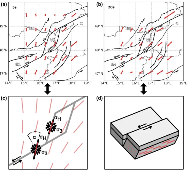
Figure

Documents relatifs
northern Zagros (3-5 mm/yr), and the Mosha fault in southern Alborz (4 mm/yr). iii) The northeastern and eastern extremities of Iran seem to belong to Eurasia. iv) The Central
The progressive counterclockwise rotation of the fast-polarization axis from eastern Anatolia to the northern Aegean might result from the addition of the
[ 7 ] The purpose of the GPS campaign was to obtain a first-order estimate of the present-day deformation in the Zagros, from stable Arabia to central Iran, across the Main
C’est ce que le Conseil d’état va conirmer expli- citement en séparant deux types de considérants : a) «considérant que l’égalité des cultes invoquées par la
The hadronic invariant mass scale uncertainty is dominated by the neutral energy and charged particle momentum scale.. Any serious discrepancy between simulation and data would
The Barlow-Proschan importance index of the system, another useful concept introduced first in 1975 by Barlow and Proschan [2] for systems whose components have continuous
Tension produces bar domains of width proportional to (lSc)-*. The initial permeability decreases and the eddy current loss increases with tension. Infinite permeability is not
u(r) is not restricted to the (( muffin-tin )> form, but obtaining solutions is difficult unless it is. The equation above is readily modified so as to describe the
