Evaluating Computational Models of Vision with Functional Magnetic Resonance Imaging

HAL Id: tel-01292787

https://tel.archives-ouvertes.fr/tel-01292787

Submitted on 23 Mar 2016

HAL is a multi-disciplinary open access

archive for the deposit and dissemination of

sci-entific research documents, whether they are

pub-lished or not. The documents may come from

teaching and research institutions in France or

abroad, or from public or private research centers.

L’archive ouverte pluridisciplinaire HAL, est

destinée au dépôt et à la diffusion de documents

scientifiques de niveau recherche, publiés ou non,

émanant des établissements d’enseignement et de

recherche français ou étrangers, des laboratoires

publics ou privés.

Functional Magnetic Resonance Imaging

Michael Eickenberg

To cite this version:

Michael Eickenberg. Evaluating Computational Models of Vision with Functional Magnetic Resonance

Imaging. Computer Vision and Pattern Recognition [cs.CV]. Université Paris Sud - Paris XI, 2015.

English. �NNT : 2015PA112206�. �tel-01292787�

ÉCOLE DOCTORALE 427 :

INFORMATIQUE PARIS SUD

Laboratoire : Equipe Parietal, Inria Saclay, CEA Saclay

THÈSE DE DOCTORAT

INFORMATIQUE

par

Michael EICKENBERG

Evaluation de modèles computationnels de la vision humaine

en imagérie par résonance magnétique fonctionnelle

Date de soutenance :

21/09/2015

Composition du jury :

Directeur de thèse : Bertrand THIRION DR, Inria Saclay, Palaiseau

Rapporteurs : Marcel VAN GERVEN DR, Donders Institute, Nijmegen, NL Nikolaus KRIEGESKORTE DR, Cambridge University, UK Examinateurs : Stéphane MALLAT Professeur, ENS, Paris

Yves FREGNAC DR, CRNS Gif-sur-Yvette, Gif-sur-Yvette Balazs KEGL DR, Université de Paris Sud, Orsay Alexandre GRAMFORT DR, CRNS, Télécom ParisTech, Paris

doctoral school of computer science

prepared at parietal team - inria saclay

Evaluating Computational Models of Vision with

Functional Magnetic Resonance Imaging

Michael Eickenberg

A dissertation submitted in partial fulfilment

of the requirements for the degree of doctor of science,

specialized in computer science.

Director: Bertrand Thirion

Co-Directors: Alexandre Gramfort, Gaël Varoquaux

Defended publicly the 21th of September 2015 in front of a jury consisting of

Advisor

Bertrand Thirion

INRIA / CEA, Saclay, France

Reviewers

Marcel Van Gerven

Donders Institute, Nijmegen, NL

Nikolaus Kriegeskorte

MRC-CBU, Cambridge University, UK

Examiners

Stéphane Mallat

ENS, Paris, France

Yves Frégnac

UNIC, CNRS, Gif-sur-Yvette, France

Balász Kégl

CNRS, Université de Paris Sud, France

Alexandre Gramfort

Telecom Paristech, Paris, France

école doctorale informatique

équipe parietal - inria saclay

Evaluation de modèles computationnels de la

vision en imagerie par résonance magnétique

fonctionnelle

Michael Eickenberg

Thèse de doctorat pour obtenir le grade de

DOCTEUR de l’UNIVERSITÉ de PARIS-SUD

Dirigée par Bertrand Thirion.

Co-dirigée par Alexandre Gramfort et Gaël Varoquaux

Présentée et soutenue publiquement le 21 Septembre 2015 devant

un jury composé de :

Directeur

Bertrand Thirion

INRIA / CEA, Saclay, France

Rapporteurs

Marcel Van Gerven

Donders Institute, Nijmegen, NL

Nikolaus Kriegeskorte

MRC-CBU, Cambridge University, UK

Examinateurs

Stéphane Mallat

ENS, Paris, France

Yves Frégnac

UNIC, CNRS, Gif-sur-Yvette, France

Balász Kégl

CNRS, Université de Paris Sud, France

Alexandre Gramfort

Telecom Paristech, Paris, France

Abstract

Computer vision studies and biological vision studies have evolved in parallel over the last century with mostly unilateral inspiration taken from biological vision and going into the engineering of computer vision systems. From the utility of edge and blob detection to the realization that a layered or hierarchical approach to abstraction can be very powerful, most of these phenomena are to be found in natural visual systems in some way or another. With the successes in computer vision brought about during the last one and a half decades, which can be subdivided into different sub-eras (see chap-ter 4), it has become a highly intriguing question to assess whether these methods can help study brain function.

The main goal of this thesis is to confront a few more or less biologically inspired computational models of vision with actual brain data. The chosen brain data acquisition modality is fMRI, since it gives a good global overview of activity at a reasonable spatial resolution.

In recovering brain activity maps for the presentation of a preferably high number of visual stimuli, we shall attempt to relate the measured activity with the vectorial representations of the stimuli generated by the computa-tional models.

Since these representations are typically very high in dimension, we need to resort to non classical statistical methods to establish a relationship be-tween the model representations and the brain data. The method for func-tional translation from the computafunc-tional model coefficients to brain activity data is kept linear. This is essential for evaluation, in order to keep most nonlinear complexity in the computational model under scrutiny, instead of adjusting for the lack of it through nonlinear estimators. However, due to the abundance of coefficients in typical computational models, the forward problem is ill-posed and calls for regularization as well as an evaluation on held-out data typical of the field of machine learning.

In chapter 2 of this thesis we will familiarize ourselves with the nature of the fMRI BOLD response by evaluating the utility of estimating the hemo-dynamic impulse response function (HRF) due to experimental stimulation. The evaluation is specifically geared towards assessing whether attention to estimating the shape of the HRF is merited in the context of machine learning forward and reverse models.

A focus on specific convex regularization techniques will be explored in chapter 3. We introduce a convex region-selecting penalty which segments smooth active sets from a uniform zero background. This spatial regularizer is applicable to the space of brain images. We will evaluate it in a reverse mod-elling setting - predicting an external variable from brain activity patterns. Here again, the number of voxels typically largely exceeds the number of ob-servations, leading to an ill-posed problem necessitating regularization. We choose to regularize by taking into account the spatial neighborhood struc-ture of brain images, because neighboring voxels tend to correlate in activity. In chapter 5 we evaluate a first forward (“encoding”) model with specific attention to the benefits of adding a layer to a convolutional filter model of vision. Indeed, one-layer filter models such as Gabor or Morlet filtering fol-lowed by rectification have been tried and tested successfully in numerous

experiments, including the notable application to fMRI by [Kay et al., 2008]. Since first layer filters represent an adequate model for lower-level brain ac-tivity such as center-surround calculations in LGN or edge detection in V1, the question is whether adding a second layer to the analysis could be bene-ficial to model fitting. Experiments were performed on two datasets: 1) Data acquired in the Parietal lab prior to this thesis - BOLD fMRI responses to the presentation of natural visual textures. 2) The dataset of [Kay et al., 2008] for a parallel analysis on natural images. We evaluated the second layer of the scattering transform [Mallat, 2012] against the first layer, which is a wavelet transform modulus (e.g. Gabor or Morlet modulus). In addition, the texture experiment also yielded itself to classical statistics: brain activation due to texture stimulation and differential brain activation between different texture classes are explored..

Recent breakthroughs in the field of convolutional networks have led to breathtaking progress in their capacity to perform tasks that were previously believed to be strongholds of human superiority over machines. Deep lay-ered convolutional architectures create progressively abstract representations of the data they analyze with increasing layer number. The first layer of a convolutional network geared towards object recognition typically learns to detect edges, other first-order texture boundaries, color boundaries and blobs - similar in essence to the functionality one may find in earliest vision. At the end of the convolutional network there are indicator channels outputting probability estimates for a certain number of object categories. These are based on linear transformations of the penultimate layer, which can thus be declared to linearize object category. In [Cadieu et al., 2014] it is shown that populations of inferotemporal neurons behave similarly. Having pinpointed similarities to biological signal processing at the beginning and at the end of the convolutional net processing hierarchy, we proceed to investigate simi-larities of the representations along the layers of the network.

Chapter 1 introduces the reader to fMRI and standard analysis methods. Chapter 4 gives an overview of computer-vision models.

Acknowledgements

At some point during the meanderings around and into the adjacent pos-sible, guided less and less by external force fields giving drift direction, the question becomes whether the movement reduces to isotropically random or picks up its own intrinsic momentum that can compensate dwindling gradi-ent information. In this situation, at one and the same momgradi-ent one can feel perfectly isolated and fully woven into the surrounding social fabric. Scaling a mountain alone through a thick layer of fog, in the hope that the peak is either attainable and high enough to be above the clouds or the clouds low enough to see from somewhere off the slope can be quite a solitary experience. On the other hand, flowing in the school-of-fish-like dynamics of the scien-tific community is a collective and immersive action. We also flow along with society at large, which acknowledges an essential part of the human condition - curiosity - and accommodates a formalized version of it, i.e. letting us do our work, not of course without expecting and reaping its own benefits. We are pretty lucky to be able to do research - to stand with one leg on the shoul-der of the scientific giants that preceded us and with the other on those many other shoulders of giants that give us the space to do what we do right now. At that level of generality there would be millions of people to thank. Here I will restrict myself to people I know, who helped me along these last years and without who I would not have come this far. My first word of thanks goes out to my thesis director, Bertrand Thirion, who guided me through one year of internship and three years of PhD, without wavering, especially through the inevitable sticky moments this first true journey into research can have. The same can be said of my co-supervisors Alexandre Gramfort and Gaël Varoquaux. All three never failed to push me forward when it was necessary and always had the right words at the right moment. The reviewers of my thesis manuscript were Marcel van Gerven and Nikolaus Kriegeskorte, whom I thank for accepting to review and for the feedback they gave me. Naturally I would also like to thank the rest of my thesis committee, which consisted of Yves Frégnac, who acted as president, Bertrand Thirion, Alexandre Gram-fort, Balazs Kégl, and Stéphane Mallat. I would like to address special thanks to Stéphane Mallat for having accompanied my work over all these years through our common ANR project and always giving very helpful feedback. This also goes for all his team members, past and present, who in addition to being extremely competent, are also the friendliest of people: Joan Bruna, Joakim Andén, Laurent Sifre, Edouard Oyallon. I’m glad to be able to con-tinue my work in this lab alongside Edouard, Mathieu Andreux, Irène Wald-spurger, Vincent Lostanlen, Sira Ferradans, Grégoire Sergeant-Perthuis and Carmine Cella. Towards the end of my internship year preceding my PhD, I was also lucky enough to be able to work on the signal processing topic of super-resolution for MEG with Alexandre Gramfort and Gabriel Peyré, who I thank for the time he took and the impressive supervision and

feed-back he gave at every discussion. I also greatly enjoyed interacting with

Samuel Vaiter, Mohammed Golbabaee, Charles Deledalle, Hugo Raguet, both at the lab and at spars2013. Next, in a brief stint of 11 days in Berkeley, I was able to meet and work with Jack Gallant’s lab, the team that made my PhD results possible by kindly providing the data of their immensely

suc-cessful encoding experiments to the public for download. I met the brightest and friendliest people ever and am very thankful to have been able to col-laborate with Alex Huth and Natalia Bilenko and to have met Jack himself, Mike Oliver, Anwar Nuñez, James Gao, Fatma Imamoglu and the rest of the team during my stay. I would like to thank my collaborators for engaging and fruitful interactions: Fabian Pedregosa, Mehdi Senoussi, Philippe Ciuciu, Danilo Bzdok, Elvis Dohmatob, Olivier Grisel, Thomas Hannagan, Kyle Kast-ner, Konstantin Shmelkov. Further shout-outs have to go to all current and former lab mates who I enjoyed all those coffee breaks with: Benoît Da Mota for all the petaflops, Yannick Schwartz for the trolling, all the driving, the drive-trolling and the troll-driving as well as some good conversations that bridged any traffic jam, Virgile Fritsch who I congratulate for his part-time 32 hour week, Viviana Siless who I congratulate for absolutely making it and for some awesome food samples. Sergio Medina, Bernard Ng, Clément Moutard, Martin Perez Guevara, Esther Lin, Salma Bougacha, Laetitia Grabot, Arthur Mensch, Kamalakar Dadi, Philippe Gervais, Solveig Badillo. Les manip’ ra-dio and nurses and the whole Neurospin subject recruitment and scanning team for making that part easy for many of us. Jaques Grobler for throw-ing discs and all the latest memes and Jaques Grobler and Svenja Lach for the SA vibes and fun at parties, Alexandre Abraham for being the essence of kindness and taking care of everything, Valentina Borghesani for also be-ing the essence of kindness and takbe-ing care of everythbe-ing, Mehdi Rahim for the same - all three incarnations of incredible real-world efficiency. Régine Bricquet for being the real-life incarnation of at least nine people in parallel with incredible real-world efficiency. Alexandre Abraham, Nicolas Chauffert, Murielle Fabre, Sandrine Lefranc, Remi Magnin, Guillaume Radecki for Por-querolles at which what happens stays. Andrés Hoyos-Idrobo, Léonard Blier, Elvis Dohmatob, Pedro Pinheiro Chagas, Loïc Esteve and Aina Frau Pascual for being awesome at ping pong. Christophe Pallier, Thomas Hannagan, Eve-lyn Eger, Alexandre Vignaud, Alexis Amadon and Aaron Schurger for very useful insights along all these years. Valentina, Laetitia and Aaron for helping me organize the Unsupervised Decoding Club for a year. Baptiste Gauthier, Yannick Schwartz, Alexandre Abraham, Marie Amalric, Murielle Fabre and actually everybody else for awesome coffee break discussions. Pedro Pinheiro Chagas for beer and Pedro and Aina for breakfast coffees. Kyle Kastner for getting me motivated to look at neural networks and Theano and Olivier and Kyle for great discussions about these topics. Charles Ollion for deep learning meetups and workshops and Charles, Kyle, Olivier, Mike, Anwar, Gaël and Danilo for good company at NIPS. Denis Engemann and Danilo for convinc-ing me that the future is well taken care of. Aina as well as Valentina and Fabian for being there in the right moments and Murielle, Aina, Valentina, Mehdi and Alex for making the thesis defense go smoothly. Of course Mar-ian, Trevor, Dana and so many others that I never lost contact with through these last four years. And of course my parents and my sister. And Kaja, for sticking through this with me until the end.

1 Introduction to functional MRI

1.1

Imaging modalities

1.2

MRI

1.3

Functional MRI

2 Data-driven HRF estimation for encoding and

de-coding in fMRI

2.1

Motivating Example

2.2

Data-driven HRF estimation for encoding and decoding models

2.3

Methods

2.4

Data description

2.5

Results

2.6

Discussion

2.7

Conclusion

2.8

Outlook

3 Combining Total Variation and Sparsity in a new

way

3.1

Introduction

3.2

Sparse Variation: A new spatially regularizing penalty

3.3

Optimization strategy

3.4

Empirical Results

3.6

Segmenting regions from MRI data

3.7

Convergence of the method

3.8

Discussion

3.9

Screening rules?

3.10 Variation Lasso

4 Computer-Vision models

4.1

Classical Computer-Vision Pipelines for Object Recognition

4.2

Artificial Neural Networks

4.3

Biologically Inspired Models

4.4

Scattering Transform

5 Analyzing human visual responses to textures

5.1

Introduction

5.2

Experimental Setup

5.3

Data analysis methods

5.4

Results

5.5

Discussion

6 Mapping the visual hierarchy with convolutional

nets

6.1

Introduction

6.2

Methods

6.3

Experimental results

6.4

Discussion

7 Conclusion

7.1

Summary

7.2

Outlook

8 Appendix

8.1

Dataset descriptions

8.2

Analytical leave-k-out ridge regression

1.1

Imaging modalities

There exist a number of techniques for the acquisition of brain activity which rely on a very diverse set of possible observable signals. In general, any signal that is sufficiently immediately generated and modulated by brain activity can serve as a tap for a brain activity acquisition method. Useful dimensions by which to taxonomize a large number of these methods are the following:

• invasiveness, i.e. to what extent the body containing the brain of interest is manipulated during the acquisition,

• spatial resolution, characterized by a minimal characteristic spatial scale below which no details can be measured,

• temporal resolution, characterized by a time scale below which no details can be measured.

It is important to note that depending on the process by which brain signal is obtained, loss of resolution can be incurred at intermediate steps. Ideally, the final measurement should reflect the intrinsic resolution of the signal due to this process, but in principle, these can be uncoupled: For example, an inher-ently slow signal can be sampled at many time points, which can potentially reduce noise, but it cannot recover any high temporal frequencies previously lost. We present an incomplete overview of methods in order to be able to situate fMRI, which this thesis makes use of, better with respect to the others.

1.1.1

Highly invasive methods

Highly invasive methods are characterized by requiring surgical intervention to enable acquisition.

Recently, several methods acquiring light images have had success. These methods include voltage sensitive die (VSD) [Tasaki et al., 1968, Orbach et al., 1985] methods, where a substance which changes color as a function of local potential electric energy is applied to the cortex, making electric brain activity visible to a camera.

Figure 1.1: VSD setup. Taken from [Grinvald, 2004]

Figure 1.2: Typical general optical

imaging setup. If there exist

con-trast agents (natural or not) that modulate light according to bio-logical function, this setup can be used to acquire images. Taken from [Hillman, 2007]

While VSDs modulate with voltage change, calcium imaging [Smetters et al., 1999] is a technique by which so-called calcium indicators, molecules that become fluorescent on calcium binding, are used to assess the calcium content of neurons, which is directly related to their activity because it con-tributes to the polarization of the cell.

In general, any contrast agent creating modulation of fluorescence or re-flectivity properties as a function of biological processes can be amenable to optical imaging methods [Hillman, 2008].

More traditionally, there is electrophysiology, for which a variety of tech-niques has been developed. The general setup requires the placement of an electrical conductor into or into the vicinity of neurons in order to measure the local voltage. Intracellular recordings are obtained when an electrode is placed inside a neuron. Local field potentials are obtained by placing an elec-trode at a sufficient and sufficiently similar distance from several neurons. The electrodes measure voltage fluctuations from neurons within a certain radius.

Figure 1.3: Schematic visualization of an intracellular recording. It is possible to place arrays of many electrodes arranged in a grid to

record from multiple locations at once. Intracranial EEG or Electrocorticog-raphy (ECOG) is a similar technique in which a plastic sheet containing more widely spaced electrodes is placed on the cortex.

Figure 1.4: Electrocorticography

electrode grid placed on the surface of the cortex of a human subject. The latter, along with depth electrodes, are also used in humans, for

ex-ample to determine the focus points of epilepsy attacks that a patient may suffer.

1.1.2

Less invasive methods

Comparing to the strongly invasive methods mentioned above, there are less invasive imaging modalities, whose degree of invasiveness owes to the use of radiation or radioactivity. Anatomical and functional brain imaging can be obtained by computed tomography (CT). Tomography is the measure-ment of projections of a 3-dimensional object with varying density onto a certain number of 2-dimensional planes. Reconstruction of the original 3-dimensional object can be done by solving an inverse problem, which is of-ten linear. In X-ray CT the measurement projections onto planes are obtained using X-ray light which is partially absorbed depending on the local prop-erties of the matter it traverses. Functional and other metabolic information can be imaged by injecting a contrast agent which the organism transports to specific sites and which change the way the X-rays are absorbed.

Figure 1.5: X-ray CT and PET scan-ner Siemens Biograph TruePoint Another form of computed tomography is Positron Emission Tomography

(PET), which is designed to track metabolic activity. A fast-decaying radio-active glucose is injected. At each radioradio-active decay, two gamma photons are emitted in opposite directions and captured outside the head. The emission of two photons is necessary to conserve momentum and makes it possible to localize brain activity.

1.1.3

Non-invasive methods

Non-invasive methods are techniques which measure brain signal and anatomy without any known potentially adverse side-effects. No surgery is required and no contrast agents are injected. Electromagnetic brain activity can be measured outside the head. Scalp electrodes can acquire an electroencephalo-gram (EEG), providing measurements at almost arbitrary temporal resolu-tion. By the non-relativistic Maxwell equations, the measurements are a lin-ear function of the total brain electric activity. Similarly, dynamic magnetic activity of the brain can be measured using superconducting SQUID sensors,

giving rise to a magnetoencephalogram (MEG). One can measure magnetic field intensity (using so-called magnetometers) as well as magnetic field gra-dient in two directions tangential to the surface (using so-called gradiome-ters). Both EEG and MEG acquisitions, by the simple fact that data acquisi-tion is performed at a distance from the signal source, act as a spatial low-pass filter, where the kernel has heavy tails and decreases as√_R2_+x2−3, where

R is a characteristic distance. 1 _{Due to the Maxwell equations this cannot}

1_{This kernel arises exactly in a}

styl-ized setting, where one studies the magnetic field evoked by sources on one straight line, measured on a parallel straight line. One observes a convolution of the source distri-bution with the kernel described here, which amounts to low-pass

filtering. See [Eickenberg, SPARS

2013, Poster 141] for details. be avoided. Even if measurements were taken continuously on a full sphere

around the head, the reconstruction problem remains ill-conditioned. Addi-tionally, for EEG, the scalp acts like a further spatial low-pass filter, aggra-vating the ill conditioning of the source reconstruction problem. In the MEG case the scalp does not act as an additional low-pass filter, making measure-ments more precise. Typically one has access to around 300 channels, all types taken together, which is more than using a normal EEG setup, which can use anywhere from very few to around 250 electrodes. The fact in both MEG and EEG that there can only be up to hundreds of electrodes due to space constraints on the scalp makes the source reconstruction problem ill-posed in addition to ill-conditioned (because there are many more candidate locations for sources than measurements). Both ill-conditioning and ill-posedness can be addressed by regularization.

Figure 1.6: Placement of EEG elec-trodes on the head.

Figure 1.7: MEG machine in a mag-netically shielded room (MSR). A further non-invasive method which relates back to the optical imaging

methods mentioned earlier is fNIRS (functional near-infrared spectroscopy). As many may have experienced, the light of a traditional flashlight, when covered by the hand, becomes a light red. This indicates permeability of tis-sue by light in the red spectrum. As it turns out, this permeability is most pronounced in the near infra-red spectrum (650nm to 1350nm). Skin, tissue and bone are almost transparent in the window of 700-900nm. However, oxy-hemoglobin and deoxy-oxy-hemoglobin have stronger absorption properties and can thus be identified. They can also be distinguished amongst each other because their absorption spectra differ. This phenomenon can be used for op-tical imaging. By using several light sources and several points of measure-ment, a forward model of light diffusion can be inverted, leading to spatial

localization at a∼1cm resolution.

Another method classified as non-invasive is Magnetic Resonance Imaging (MRI). Since this is the acquisition modality employed in this thesis, it will be described in a separate section.

1.2

MRI

Magnetic resonance imaging is based on Nuclear Magnetic Resonance (NMR). This non spatially specific effect is then exploited to obtain a spatial image.

1.2.1

Nuclear magnetic resonance

A proton2placed in a homogeneous magnetic field will align its spin with

2_{In general, an atom or molecule}

with non-zero net spin the magnetic field vector. Energy introduced in the form of a radio frequency

(RF) pulse can cause the proton to be excited into precession around its axis. The proton dissipates this energy by emitting radio waves at its precession frequency until it has returned into alignment with the magnetic field.

Cru-cially, the precession frequency, called the Larmor frequency, is proportional to the magnetic field to which the proton is exposed.

The above description relies on concepts from classical physics, but the quantum mechanical description is similar: The application of a magnetic field splits the ground energy state of a proton into two possible states. The energy gap between the states is proportional to the magnetic field and thus an RF pulse containing photons of the corresponding frequency can excite the protons into the antiparallel state. The proton decays back into its ground state with a probability following an exponential law with a certain half-life, emitting the acquired energy in a photon with the Larmor frequency. This effect was first described in 1938 by Isidor Rabi, based on the Stern-Gerlach experiment. In the late 40s this technique was extended to liquids and solids, independently by Felix Bloch and Edward Mills Purcell.

Figure 1.8: NMR spectrometer

for the study of the structure of molecules via quantum magnetic effects such as Zeeman energy level splitting.

1.2.2

Magnetic Resonance Imaging

Magnetic Resonance Imaging (MRI) exploits the fact that nuclear magnetic resonance frequency has such a simple dependence on the intensity of the magnetic field surrounding the nucleus. Producing a linear change in mag-netic field intensity (not orientation) along a given axis in 3D space makes all hyperplanes perpendicular to the change direction have the same magnetic field intensity, leading to the same Larmor frequency for protons lying upon it. This fact permits selective excitation of 2D slices in 3D space, since it is possible to send an RF pulse in a prescribed frequency range, using a cardinal sine (sinc) waveform_sin(πωt)/(πωt). In order to acquire an image of a 3D object, one may now consider the simpler problem of acquiring it slice by slice. However, the excitation of a full slice will lead to the simultaneous de-cay of excitation over all of the slice at the same Larmor frequency, rendering localization of activation impossible. To address this issue, spatial gradients along the slicing plane are put in place after the slice has been excited, leading to a variation of Larmor frequency across the slice. One can apply a linear gradient of different intensities in two directions along the slice. Measure-ment of the emitted RF signal for a given configuration of gradients yields a sum of signals over varying Larmor frequencies. When applying two linear gradients in perpendicular directions across the slice it is impossible to avoid identical Larmor frequencies on a set of parallel lines. These lines are in fact hyperplanes to the gradient intensity vector. Measuring the nuclear RF signal of a slice in many different constellations of linear gradient, usually on an equally spaced grid of gradient intensities, makes it possible to disambiguate the signal from specific spatial locations which all summed into these fac-tors. The space of possible gradient intensity vectors is called k-space, and by virtue of the fact that the measured RF signal is a linear superposition of sig-nal at different frequencies, the acquired k-space sigsig-nal conveniently is equal to the Fourier transform of the spatial signal. By applying a simple inverse Fourier transform, the spatial structure of the slice can be recovered.

Figure 1.9: Example of a k-space

trajectory for the measurement of an EPI image

• T1 is the characteristic time scale on which excited protons fall back into

the ground state, aligned with the homogeneous magnetic field. Also

called spin-lattice decay, it indicates the time by which the longitudinal

magnetization.

• After a so-called 90-degree-pulse, which excites around half the protons, leading to a net longitudinal magnetization of 0 and a synchronization in the xy-plane, due to material-intrinsic local field inhomogeneities the spins dephase, leading to an exponential decrease of the net xy-plane magneti-zation. T2 is the characteristic time of this decay type.

• T2* is similar to T2 decay but due to extrinsic magnetic field inhomo-geneities, for example blood flow. This relaxation type gives rise to the BOLD signal.

Depending on the timing of the measurements and the gradient pulses ap-plied, the measured image can be dominated by different types of signal decay. T1-weighted images are typically used for anatomical imaging and T2-weighted images are used to create the BOLD contrast.

Initially, typical acquisitions proceeded by exciting a slice via an RF pulse, placing a series of spatial gradients and possibly other RF pulses, followed by measurement of the emitted radio frequency signal after a certain time of evolution. Echo-planar imaging [Stehling et al., 1991] was introduced later and relies on the fact that several gradient positions can be measured with only one slice excitation, permitting a much faster sweep of k-space and an order of magnitude of acquisition speed improvement.

A typical MRI scanner consists of a superconducting hollow cylindrical magnetic coil carrying a magnetic field of between 1.5T and 7T parallel to the axis of the cylinder. For human MRI machines the cylinder is oriented horizontally. The axis of the cylinder is called the z-axis, elevation is the y axis and the remaining left-right axis is called x. The z-axis gradient is created by a pair of Helmholtz coils placed at either ends of the cylinder. The x- and y-gradients are created by pairs of half-cylinder coils acting in an opposing manner.

Figure 1.10: Clinical MRI machine

1.3

Functional MRI

Most modern functional MRI acquisitions rely upon the BOLD effect. It will be briefly introduced before a review of typical experimentation types done with this signal.

1.3.1

Blood Oxygen Level Dependent signal

In 1989, Ogawa and collaborators made a finding that should revolutionize the way brain function is measured [Ogawa and Lee, 1990]. They discov-ered hemoglobin as a natural contrast agent in T2*-weighted imaging. Since hemoglobin is directly involved in the oxygen supply within the body, this contrast can measure metabolic activity in the brain. Following neural activ-ity and depletion of energy, the active region is supplied with fresh blood in a localized manner. Immediately following neural stimulation, the concentra-tion of deoxyhemoglobin rises, followed by an onrush of more than necessary oxyhemoglobin. Deoxyhemoglobin is paramagnetic, whereas oxyhemoglobin is diamagnetic. These are different susceptibility properties which lead to

different behavior when these materials are placed in a magnetic field: dia-magnetic materials give rise to a dia-magnetic field which counteracts the one in which they are placed, leading to a local net-reduction of magnetic field. Paramagnets act the opposite way by contributing in the direction of an ex-ternally applied magnetic field.

Thus oxygen level as a metabolic indicator becomes visible to MRI. While the full mechanism of neuro-vascular coupling is still not fully understood, direct links to neural activity have been established [Logothetis et al., 2001].

Since however the BOLD response is a mixture of cerebral blood flow, cerebral blood volume and cerebral metabolic rate of oxygen changes, it is a relative measure without a baseline. In certain settings this necessitates the interpretation of a contrast of two images instead of the images themselves.

Apart from extreme cases, the BOLD response is approximately linear in the underlying neural activity. Given a train of stimulative or behavioral events it has also been put forward and tested that the BOLD response, within a certain range, acts like a linear time-invariant system (LTI) [Boynton et al., 1996]. As a consequence, the response of a given brain voxel to a function of neural activity and events is fully characterized by the convolution of the neural activity function with a causal finite impulse response function, gen-erally named the hemodynamic response function (HRF).

With MRI scanners available in many hospitals and research institutions, the discovery of the BOLD signal gave cognitive scientist a relatively cheap, reliable and spatially well-resolved tool to examine brain function. The ex-plosion in number of publications pertaining to fMRI studies confirms this [Poldrack et al., 2011a].

1.3.2

fMRI experiment types

Different ways of studying the brain with fMRI have been established and been given category names. A major difference in brain activity can be ob-served between the brain engaged in a specific task and the brain at rest. The latter type of experiment requires the subject to engage in nothing but pos-sibly mind-wandering. This can be done eyes open or eyes closed without visual stimulation. A rich body of literature exists around resting state fMRI. A notable discovery using fMRI has been the default mode brain network, which seems to be strongly active during rest periods [Raichle et al., 2001].

The other type of experiment is task-related. Given a cognitive task or ex-ternal stimulation, brain activity specific to it will be elicited and can be con-trasted against appropriately chosen control conditions in which the studied brain function is presumably inactive.

Different types of experiments include the presentation of visual, auditory or sensory stimulation either in passive perception or with active tasks such as memory, attention, discrimination or decision tasks. Underlying the design of high-level cognitive tasks there is often a mechanism of testing one theory against another, by choosing situations in which they would yield different predictions.

An fMRI experiment with stimulation and/or tasks is typically set up ei-ther as an event-related or a block design. In an event-related design, neural activity is elicited in brief singular events which can be visualized on a graph

as spikes. They lead to a hemodynamic response consisting of the superpo-sition of HRFs time-locked to the events (provided these are not spaced too closely, incurring a violation of the LTI model). In a block design, neural activity is elicited during extended periods of time, for example by showing different images of a same category. The stimulus may change in order to sustain neural activity, but the activation will be considered as one block and averaged. The neural activation functions can be visualized as boxcar func-tions (this is the case e.g. in [Haxby et al., 2001]). When convolved with the hemodynamic response function, they give rise to a shifted version of the boxcar with slightly smoothed edges.

1.3.3

Statistical methods for fMRI data analysis

Functional MRI is an imaging modality in which raw images are uninter-pretable or at least very difficult to interpret by the human eye. Effect sizes are small with respect to baseline signal: BOLD signal changes typically amount to 5% of the mean image and the signal to noise ratio is low - typically around 0.1. This situation makes statistical analysis indispensible even for qualitative analysis as activation is indistinguishable from non-activation by looking at the raw signal.

Preprocessing

Before any analysis can be done on fMRI data, a number of preprocessing steps needs to be taken. A typical experimental acquisition session involves an anatomical scan, using a T1-weighted image. This anatomical image per-mits a segmentation into different tissue types, such as white matter and gray matter. Cerebro-spinal fluid (CSF) and skull or the rest of the head are also

segmented. If coregistered with a functional acquisition, this permits the

identification of gray-matter voxels in the functional images.

During functional scanning over a length of time, head movement is al-most unavoidable. In motion correction or realignment, each acquired func-tional image is transformed to match a reference image (taken, e.g. from the middle of the acquisition), using strictly rigid body transforms, which can be parametrized by a translation and a 3D rotation. This assumption encodes the fact that we do not expect the brain to change shape or size during the ac-quisition. Since the alignment is done between images of the same type, one

can expect that a well-aligned image should incur minimal`2or correlation

error. This is the cost function that is usually optimized in the transformation parameters.

An optional preprocessing step is slice-timing correction. In effect, due to the fact that the 3D images are acquired by slices, one by one, the time of the acquisition of each slice is different. Further, adjacent slices may not be acquired at adjacent points in time. In interleaved acquisition and in multi-band acquisitions, this is not the case. It is straightforward to see that the slice timing delay relative to the neural event onset will cause a shift in the sampling of the hemodynamic response. If using methods that are rigid in their assumptions of the HRF, and brain volume acquisition takes more than TR=2s, then slice-timing correction may be a useful preprocessing step. It is done by temporal interpolation, where the type of interpolation needs to be

chosen. Temporal sinc interpolation yields the least biased results at the cost of needing more filter taps than e.g. a linear or quadratic interpolation.

It is also possible that fMRI acquisitions incur artefacts such as ghosting or spikes. Visual scrutiny or analysis using ICA or simple temporal differen-tial analysis summaries can give indications as to the locations of spikes and corresponding volumes.

After these steps, which are often referred to as minimal preprocessing, we are ready to perform fMRI statistics, basing ourselves on the hypothesis or fact that now a given voxel refers to the same part of the brain throughout the analysis.

FMRI signal has several properties that need to be taken into account in order for analysis not to fail. First and foremost there are the low-frequency drifts which dominate the norm of the signal and have been essentially char-acterized as nuisance variables. Importantly, the information recoverable by an fMRI analysis resides in the high frequencies or must reside in the high frequencies, because otherwise it is confoundable with drifts and discarded when drifts are discarded. As a consequence, when designing an experiment, one must be careful not to include effects that are too slow. A typical cutoff

for drift frequency is_{1/128Hz. Drifts can be removed by high-pass filtering}

through projecting onto high-frequency Fourier coefficients. One can also use global or local polynomials up to a certain degree, as they enforce slow vari-ation. For local polynomial smoothing the Savitzky-Golay filter has turned out helpful. Drifts can be removed either before statistics or accommodated for in statistical estimation.

Another issue that needs to be taken into account is noise. Noise is gen-erally so strong that it is impossible to see the BOLD-induced signal change in one image by eye. It must be included at least implicitly into any data analysis model put forward. One can choose a white Gaussian model, but an autoregressive model with a one-timepoint history has also been successfully employed.

GLM

In the General Linear Model (GLM), voxel activations due to experimental conditions are written as the noisy linear forward model

y=Xβ+ε,

where_{X represents in its columns the event or condition regressors, which,}

exploiting the LTI model, are indicators of neural activity convolved with the hemodynamic response. These different regressors are weighted by the en-tries of the β-vector and the noise vector is added. Assuming white Gaussian

noise ε with zero mean and variance σ2and full column rank of_{X, the best}

unbiased estimator for β is

ˆβ=X+y=β+X+ε.

The new noise term_X+_{ε is still Gaussian with zero mean.}

After performing the GLM, we are usually interested in establishing a rel-ative difference measure between two or more conditions, in the form of a statistical contrast. Let(ei)ibe unit vectors and suppose we are interested in

contrasting condition_{i with condition j. Then with c} = ei−ej, we would

like to infer whether the null-hypothesis that_cTβ =0 can be rejected. We

have

cTβ=cTˆβ−cTX+ε,

which is a Gaussian variableN (cTˆβ, σ√cT_X+_X+,T_{c) = N (c}T_{ˆβ, σpc}T_(XT_X)−1_c).

It is then straightforward to determine the probability of reaching the mean of this distribution with a distribution of the same variance centered at zero.

A succinct test statistic is _z = √ cTˆβ

cT_(XT_X)−1_cσ, which is the z-score of the

normal distribution.

It is to be noted that we normally do not have access to σ and have to estimate it in the model. This can be done by observing that an estimate can be obtained in the GLM residuals:

r=y−X ˆβ= (Id−XX+)ε,

which leads to krk2 ₌

ε(Id−XX+)ε = (n−p)ˆσ2, where X ∈ Rn×p

and the_n−p scaling due to the loss in degrees of freedom incurred by the

orthogonal projection. Using _{ˆσ in the above equation}

t= c

T_ˆβ

pcT_(XT_X)−1_{c ˆσ}

gives us a t-statistic on which we can perform the same inference.

Unsupervised methods

When there is no task, behavior or stimulation and the brain is scanned while resting or mind-wandering, there is still intriguing structure in the resulting signal. One method to obtain brain activation maps and their activations as time courses is Independent Components Analysis (ICA). This supposes that

the signal is a linear combination_{A of underlying sources s, which are}

max-imally statistically independent. In order to function, ICA requires at least as many samples as there are dimensions in the data. Since fMRI data are very high-dimensional and typically scarce in the sense that there are much more voxels per image than images, one resorts to discovering independent

timecourses instead of independent activation maps. The matrix of

time-courses has the correct shape proportions and the resulting ICA will show which latent timecourse components were active in which voxel. The map of each latent factor is usually spatially coherent even though by construction it contains no spatial information apart from a (crucial) smoothing before estimating the components. Another approach, this time with a focus on spa-tially contiguous and sparse activation maps is known as “TV-l1 multi-subject dictionary learning” (TV-MSDL), see [Abraham et al., 2013] for details. Both approaches give rise to clean maps than can be further segmented into re-gions if desired. A typical analysis performed on resting state data is the study of interactions between such regions. One can also obtain regions us-ing an anatomical atlas. One can for example tell apart disease condition from normal condition by classifying the covariance matrices, where disease condition can be e.g. autism or schizophrenia.

Encoding and Decoding

Encoding and Decoding, as introduced in [Naselaris et al., 2011] describe a direction in which modeling is performed. Encoding models, also known as forward models, are aligned with the direction of causality as far as possible. In an fMRI experiment, this means that the brain response is predicted from the stimulus. The way it is advocated in [Naselaris et al., 2011] is to make use of simple linear models on top of an arbitrarily complicated and nonlinear representation of the stimulus. If an encoding model of this type can explain brain activity well, it is an indication of the usefulness of the underlying non-linear representation. These models can advance the understanding of brain function. Decoding models, or inverse models, perform inference in the op-posite direction: E.g. given a brain image, a decoding model attempts to infer information about the stimulus. Often the output is chosen to be categorical, e.g. an object category seen on the screen, but can also be continuous and potentially multi-dimensional. Uses of this modeling direction arise e.g. in brain-computer interfaces, where brain state is used to control a machine, or potentially for medical diagnosis for the prediction of a disease phenotype.

Ringing implicitly within the mention of encoding and decoding models is method of evaluation. While one may reasonably argue that an encod-ing model is nothencod-ing other than a potentially ill-posed way of performencod-ing a GLM, usually the evaluation criteria are quite different. While the classical GLM is amenable to classical statistics, due to the full column rank of the

design matrix_{X, the evaluation of an encoding model is better seen as the}

evaluation of a modern machine learning method, which calculate predictive performance on unseen data. This way, even if the design matrix is singular due to an abundance of feature columns, modeling capacity can be quantified. Decoding models are evaluated analogously – also by an accuracy measure on held-out data.

encoding and decoding in fMRI

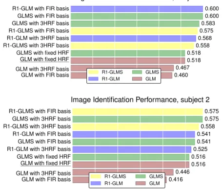
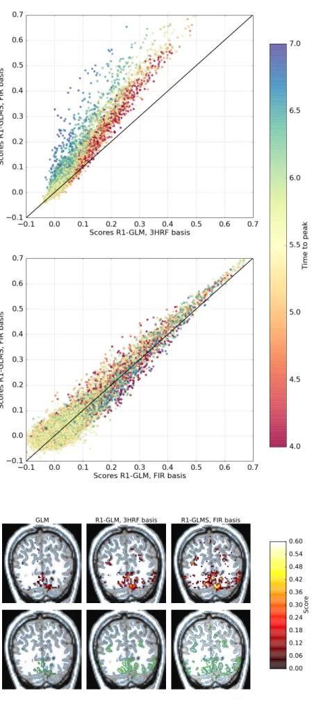
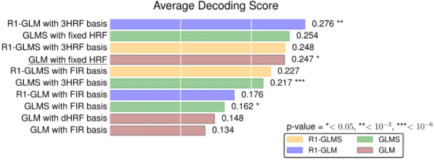
Despite the common usage of a canonical, data-independent, hemodynamic response function (HRF), it is known that the shape of the HRF varies across brain regions and subjects. This suggests that a data-driven estimation of this function could lead to more statistical power when modeling BOLD fMRI data. However, unconstrained estimation of the HRF can yield highly unsta-ble results when the number of free parameters is large. We develop a method for the joint estimation of activation and HRF by means of a rank constraint, forcing the estimated HRF to be equal across events or experimental condi-tions, yet permitting it to differ across voxels. Model estimation leads to an optimization problem that we propose to solve with an efficient quasi-Newton method, exploiting fast gradient computations. This model, called GLM with Rank-1 constraint (R1-GLM), can be extended to the setting of GLM with sep-arate designs which has been shown to improve decoding accuracy in brain activity decoding experiments. We compare 10 different HRF modeling meth-ods in terms of encoding and decoding score on two different datasets. Our results show that the R1-GLM model outperforms competing methods in both encoding and decoding settings, positioning it as an attractive method both from the points of view of accuracy and computational efficiency.

In the next section, we provide an example motivating the study of HRF estimation techniques. The subsequent sections have been published in the Neuroimage journal.

Sections 2.2 to 2.7 have been published in

• F. Pedregosa, M. Eickenberg, P. Ciuciu, B. Thirion, A. Gramfort “Data-driven HRF estimation for encoding and decoding models”, NeuroImage, Volume 104, 1 January 2015, Pages 209-220.

• F. Pedregosa, M. Eickenberg, B. Thirion, and A. Gramfort, “HRF estimation improves sensitivity of fMRI encoding and decoding models”, Proc. 3rd International Workshop Pattern Recognition in NeuroImaging, 2013

2.1

Motivating Example

The BOLD hemodynamic response to a stimulus is a complicated mecha-nism, dependent on the oxygen consumption following energy release due to neural activity, but also mechanical properties of blood flow and the blood vessels by which it is transported. It is thus somewhat surprising that linear time invariant systems modeling does capture the BOLD response quite well, provided that certain conditions on the inter-stimulus interval are met. This property is studied in [Boynton et al., 1996]. However, when consecutive stimuli are placed too close together temporally, at e.g less than 2 seconds, then the system does not satisfy the superposition property. This can be seen e.g. by considering a higher order Volterra expansion of the hemodynamic response: In the quadratic term one observes nontrivial binary interactions when stimuli are very close [Friston et al., 2000].

In this chapter we focus on the modeling of BOLD response in the frame-work of a linear time-invariant system only, e.g. sytems equal to their own Volterra expansion of first order, where we assume stimulation as impulse-like input and BOLD signal is the filtered response (the convolution with the hemodynamic impulse response function). In this context it is crucial to be able to characterize the impulse response of the system since otherwise the estimation of activity can be completely misguided.

In figure 2.1 we can see a depiction of two impulse sequences describing stimulus events for two experimental conditions. Both stimulus event trains yield a hemodynamic response whose superposition yields the full BOLD re-sponse. If this signal is analyzed with the “wrong” impulse response function (peak shifted from 6 seconds to 4 seconds), then the estimated activations can become very wrong. In this specific case they do not even preserve order.

Slightly more formally, we can write the event sequences as trains of Dirac deltas Em(t) = Nm

∑

where_{m represents different experimental conditions and the tm,n} indicate

the event times for condition_m.

Given an HRF h(t) which is assumed to have finite temporal support

[0, Lh], the regressors used in a GLM are then the convolution of the Em

event trains with the HRF:

Xm(t) =Em∗h(t) = Nm

∑

n=1

h(t−tm,n) (2.2)

The BOLD signal in one voxel is then modeled as a linear combination of these regressors: y(t) = M

∑

−_∞f(t)g(t)dt andkfk2= hf , fi(for finite numbers

of events these integrals clearly exist), given a BOLD signal _y(t)the least squares estimate is written

ˆβ=arg min_β1 2ky(t) − M

∑

0 10 20 30 40 condition 1 time/s 0 10 20 30 40 condition 2 time/s 0 10 20 30 40 condition 1 _time/s 0 10 20 30 40 condition 2 time/s 0 10 20 30 40 aggregate time/s 0 10 20 30 40 wrong HRF time/s 0 10 20 30 40 wrong HRF time/s peak at 6s peak at 4s

true activations estimated withcorrect HRF estimated withwrong HRF

Figure 2.1: Time series of events

convolved with an HRF. If a dif-ferent HRF is used for activation estimation, then activation

differ-ences can flip signs. At the top

we see event trains for two dif-ferent conditions, which are differ-ently activated (cond blue > cond red) for a chosen voxel. The second set of plots shows the event trains convolved with a hemodynamic re-sponse function peaking at 6s. Dot-ted lines show responses of individ-ual events. The third plot shows the total activity of the voxel due to the events (black line). The fourth plot shows the total activity and event responses using an HRF that peaks at 4s (“the wrong HRF”). The fifth plot shows in magenta the best fit obtainable with the HRF peaking at 4s. The last line shows that the es-timated activation maps for condi-tion blue<condition red, inverting the order of the two.

Letting _Gl,m = hXl, Xmi be the Gram matrix and cm = hXm, yi be

the inner product similarity between regressors and BOLD time course, the solution to the least squares problem can be written as

ˆβ=G−1c (2.5)

Assuming now that we have two conditions and that the BOLD activity

was generated using a “ground truth” HRF_h(t), we assess what happens if

the activity is estimated using a different underlying HRF_g(t). Let Xhm(t) = Em∗h(t)

Xgm(t) = Em∗g(t)

G_l,mg,g = hX_lg, Xgmi

G_l,mg,h = hX_lg, Xh_mi

and the BOLD signal generated as _y(t) = _∑mβmXmh(t). Then using the

HRF_g(t)leads to the following estimation of activity: ˆβg 1 ˆβg 2 ! = (Gg,g)−1Gg,hβ= hX g 1, X g 1i,hX g 1, X g 2i hX₂g, X₁gi,hX₂g, X₂gi !−1 hXg₁, X₁hi,hX₁g, X₂hi hXg₂, X₁hi,hX₂g, X₂hi ! β (2.6) In order to evaluate this estimation, we need to take a closer look at the scalar products involved. We exploit the fact that these can be written as a convolution evaluated at 0 and can then use associativity and commutativity

properties of the convolution. Using the notation ˇ_{f : x} 7→ f(−x) we can

write:

hXmg, Xhli =X g

m∗Xˇhl(0) = (Em∗g) ∗ (Eˇl∗ˇh)(0) = (Em∗Eˇl) ∗ (g∗ˇh)(0)

(2.7) The rule for the convolution of Diracs gives us(Em∗Eˇl)(t) =∑n,kδ(t−

(tm,n−tl,k)). Since the support ofg∗ˇh is[−Lh, Lg], if the events are spaced

at a larger inter-stimulus interval than_max(Lg, Lh), the scalar product

re-duces to hXgm, Xlhi = Nmδml(g∗ˇh)(0) = Nmδmlhg, hi. The estimated

activations then become

ˆβm =

hg, hi

hg, giβm, (2.8)

If the hemodynamic responses to events do not significantly overlap (i.e. the events are sufficiently tem-porally separated), then using the wrong HRF for estimation merely leads to the activation maps being scaled by a factor.

and we conclude that using the “wrong” hrf in the absence of response overlap merely results in a rescaling of activation maps. In the context of two different event types, let us assume that event 2 follows event 1 after half of the duration of the hemodynamic response and that event 1 occurs periodically with inter-stimulus interval equal to the length of the HRF. Then, with the shorthandhg, hit= (g∗ˇh)(t), we obtain

hX₁g, Xh₂i = hX₂g, Xh₁i = Nhg, hiL 2 hX₁g, Xh₁i = hX₂g, Xh₂i = Nhg, hi0 We thus obtain ˆβg 1 ˆβg 2 ! = hg, gi0,hg, giL2 hg, giL 2,hg, gi0 !−1 hg, hi0,hg, hiL 2 hg, hiL 2,hg, hi0 ! β

Assume for simplicity that the HRFs_{g, h are step functions, for example} g=q2_L1_[L 2,L] and_h=q_L21_[0,L 2] . In this casehg, gi = hh, hi = hg, hiL 2 =

1 and the other values are equal to 0, leading to If the HRF used for estimation is

radically different from the HRF

generating the signal, and the

events are unfortunately placed, then activation contrasts can flip

sign. In the constructed example

here, the two conditions exchange activation maps. ˆβg₁ ˆβg₂ ! = 1 0 0 1 !−1 0 1 1 0 ! β= β2 β1 ! ,

leading to an exact switching of activations. In practice the effect may not be as clear cut, but figure 2.1 shows an example with plausible HRFs, where the order of the strengths of the weights is inverted.

In the following, we will make the case for an HRF estimation per voxel in the context of encoding and decoding models. Indeed, most efforts of de-coding brain state from fMRI data use a deconvolution step in the form of an event related GLM in order to extract the activation coefficients β, instead of learning predictive models directly on BOLD signal (some exceptions exist and will be mentioned). We will show that the estimation of the hemody-namic response function per voxel aids both forward and reverse modeling techniques, from stimulus to brain activity and back.

2.2

Data-driven HRF estimation for encoding and

decod-ing models

The use of machine learning techniques to predict the cognitive state of a subject from their functional MRI (fMRI) data recorded during task perfor-mance has become a popular analysis approach for neuroimaging studies over the last decade [Cox and Savoy, 2003, Haynes and Rees, 2006]. It is now commonly referred to as brain reading or decoding. In this setting, the BOLD signal is used to predict the task or stimulus that the subject was per-forming. Although it is possible to perform decoding directly on raw BOLD signal [Mourão Miranda et al., 2007, Miyawaki et al., 2008], the common ap-proach in fast event-related designs consists in extracting the activation coef-ficients (beta-maps) from the BOLD signal to perform the decoding analysis on these estimates. Similarly, in the voxel-based encoding models [Kay et al., 2008, Naselaris et al., 2011], the activation coefficients are extracted from the BOLD signal, this time to learn a model to predict the BOLD response in a given voxel, based on a given representation of the stimuli. In addition, a third approach, known as representational similarity analysis or RSA [Kriegeskorte et al., 2008a] takes as input the activation coefficients. In this case a compar-ison is made between the similarity observed in the activation coefficients, quantified by a correlation measure, and the similarity between the stimuli, quantified by a similarity measure defined from the experimental setting.

These activation coefficients are computed by means of the General Linear Model (GLM) [Friston et al., 1995]. While this approach has been successfully used in a wide range of studies, it does suffer from limitations [Poline and Brett, 2012]. For instance, the GLM commonly relies on a data-independent canonical form of the hemodynamic response function (HRF) to estimate the activation coefficient. However it is known [Handwerker et al., 2004, Badillo et al., 2013b] that the shape of this response function can vary substantially

across subjects and brain regions. This suggests that an adaptive modeling of this response function should improve the accuracy of subsequent analysis.

To overcome the aforementioned limitation, Finite Impulse Response (FIR) models have been proposed within the GLM framework [Dale, 1999, Glover, 1999]. These models do not assume any particular shape for the HRF and amount to estimating a large number of parameters in order to identify it. While the FIR-based modeling makes it possible to estimate the activation coefficient and the HRF simultaneously, the increased flexibility has a cost. The estimator is less robust and prone to overfitting, i.e. it may generalize badly to unseen data. In general, FIR models are most appropriate for studies focused on the characterization of the shape of the hemodynamic response, and not for studies that are primarily focused on detecting activation [Pol-drack et al., 2011b]

Several strategies aiming at reducing the number of degrees of freedom of the FIR model - and thus at limiting the risk of overfitting - have been proposed. One possibility is to constrain the shape of the HRF to be a linear combination of a small number of basis functions. A common choice of basis is formed by three elements consisting of a reference HRF as well as its time and dispersion derivatives [Friston et al., 1998], although it is also possible to compute a basis set that spans a desired function space [Woolrich et al., 2004]. More generally, one can also define a parametric model of the HRF and estimate the parameters that best fit this function [Lindquist and Wager, 2007]. However, in this case the estimated HRF may no longer be a linear function of the input parameters.

Sensitivity to noise and overfitting can also be reduced through regular-ization. For example, temporal regularization has been used in the smooth FIR [Goutte et al., 2000, Ciuciu et al., 2003, Casanova et al., 2008] to favor solutions with small second order time derivative. These approaches require the setting of one or several hyperparameters, at the voxel or potentially at the parcel level (if several voxels in a pre-defined parcel are assumed to share some aspects of the HRF timecourse). Even if efficient techniques such as generalized cross-validation [Golub et al., 1979] can be used to choose the regularization parameters, these methods are inherently more costly than basis-constrained methods. Basis-constrained methods also require setting the number of basis elements; however, this parameter is not continuous (as in the case of regularized methods), and in practice only few values are ex-plored: for example the 3-element basis set formed by a reference HRF plus derivatives and the FIR model. This paper focuses on basis-constrained reg-ularization of the HRF to avoid dealing with hyperparameter selection with the goal of remaining computationally attractive. A different approach to increase robustness of the estimates consists in linking the estimated HRFs across a predefined brain parcel, taking advantage of the spatially dependent nature of fMRI [Wang et al., 2013]. However, hemodynamically-informed parcellations [Chaari et al., 2012, Badillo et al., 2013a] rely on the computa-tion of a large number of estimacomputa-tions at the voxel or sub-parcel level. In this chapter we focus on voxel-wise estimation methods.

We propose a method for the simultaneous estimation of HRF and ac-tivation coefficients based on low-rank modeling. Within this model, and as in [Makni et al., 2008, Kay et al., 2008, Vincent et al., 2010, Degras and

Lindquist, 2014], the HRF is constrained to be equal across the different con-ditions, yet permitting it to be different across voxels. Unlike previous works, we formulate this model as a constrained least squares problem, where the vector of coefficients is constrained to lie within the space of rank one matri-ces. We formulate the model within the framework of smooth optimization and use quasi-Newton methods to find the vector of estimates. This model was briefly presented in the conference paper [Pedregosa et al., 2013]. Here we provide more experimental validation and a more detailed presentation of the method. We also added results using a GLM with separate designs [Mum-ford et al., 2012]. Ten alternative approaches are now compared on two pub-licly available datasets. The solver has also been significantly improved to scale to full brain data.

The contributions of this chapter are two-fold. First, we quantify the im-portance of HRF estimation in encoding and decoding models. While the ben-efit of data-driven estimates of the HRF have already been reported in the case of decoding [Turner et al., 2012] and encoding approaches [Vu et al., 2011], we here provide a comprehensive comparison of models. Second, we eval-uate a method called GLM with Rank-1 constraint (R1-GLM) that improves encoding and decoding scores over state-of-the-art methods while remaining computationally tractable on a full brain volume. We propose an efficient algorithm for this method and discuss practical issues such as initialization. Finally, we provide access to an open source software implementation of the methods discussed in this chapter.

Notation: _{k · k}and _{k · k∞} denote the Euclidean and infinity norm for

vectors. We use lowercase boldface letter to denote vectors and uppercase boldface letter to denote matrices. _{I denotes the identity matrix, 1n}denotes

the vector of ones of size _n,⊗denotes the Kronecker product and_vec(A)

denotes the concatenation of the columns of a matrix_{A into a single column}

vector. _A† denotes the Moore-Penrose pseudoinverse. Given the vectors

{a1, . . . , ak}with ai ∈ Rn for each1 ≤ i ≤ k, we will use the notation

[a1, . . . , ak] ∈ Rn×k to represent the columnwise concatenation of the k

vectors into a matrix of size_n×k. We will use Matlab-style colon notation

to denote slices of an array, that is_x(1 : k)will denote the first_{k elements of}

x.

2.3

Methods

In this section we describe different methods for extracting the HRF and ac-tivation coefficients from BOLD signals. We will refer to each different ulus as condition and we will call trial a unique presentation of a given

stim-ulus. We will denote by_{k the total number of stimuli, y} ∈ Rn _{the BOLD}

signal at a single voxel and_{n the total number of images acquired.}

The General Linear Model

The original GLM model [Friston et al., 1995] makes the assumption that the hemodynamic response is a linear transformation of the underlying

neu-ronal signal. We define the_n×k-matrix XGLM as the columnwise stacking

HRF [Boynton et al., 1996, Glover, 1999] with the stimulus onsets for the given condition. In this work we used as reference HRF the one provided by the

software SPM 8 [Friston et al., 2011]. Assuming additive white noise,_n≥ k

and_XGLMto be full rank, the vector of estimates is given by ˆβGLM =X†GLMy,

where ˆβGLM is a vector of sizek representing the amplitude of each one of

the conditions in a given voxel.

A popular modification of this setting consists in extending the GLM de-sign matrix with the temporal and width derivatives of the reference HRF. This basis, formed by the reference HRF and its derivatives with respect to time and width parameters, will be used throughout this work. We will refer to it as the 3HRF basis. In this case, each one of the basis elements is con-volved with the stimulus onsets of each condition, obtaining a design matrix of size_n×3k. This way, for each condition, we estimate the form of the HRF as a sum of basis functions that correspond to the first order Taylor expansion of the parametrization of the response function. Another basis set that will be used is the Finite Impulse Response (FIR) set. This basis set spans the com-plete vector space of dimension corresponding to the length of the impulse response and it is thus a flexible model for capturing the HRF shape. It con-sists of the canonical unit vectors for the given duration of the estimated HRF. Other basis functions such as FMRIB’s Linear Optimal Basis Sets [Woolrich et al., 2004] are equally possible but were not considered in this work.

More generally, one can extend this approach to any set of basis

func-tions. Given the matrix formed by the stacking of _{d basis elements B} =

[b1, b2, . . . , bd], the design matrix XB is formed by successively stacking

the regressors obtained by convolving each of the basis elements with the

stimulus onsets of each condition. This results in a matrix of size _n×dk

and under the aforementioned conditions the vector of estimates is given by ˆ

β_B = X†_By. In this case, ˆβ_Bis no longer a vector of size _{k: it has length}

k×d instead and can no longer be interpreted as the amplitude of the

acti-vation. One possibility to recover the trial-by-trial response amplitude is to select the parameters from a single time point as done by some of the models considered in [Mumford et al., 2012], however this procedure assumes that the peak BOLD response is located at that time point. Another possibility is to construct the estimated HRF and take as amplitude coefficient the peak amplitude of this estimated HRF. This is the approach that we have used in this paper.

GLM with rank constraint

In the basis-constrained GLM model, the HRF estimation is performed in-dependently for each condition. This method works reliably whenever the number of conditions is small, but in experimental designs with a large num-ber of conditions it performs poorly due to the limited conditioning of the problem and the increasing variance of the estimates.

At a given voxel, it is expected that for similar stimuli the estimated HRF are also similar [Henson et al., 2002]. Hence, a natural idea is to promote a common HRF across the various stimuli (given that they are sufficiently similar), which should result in more robust estimates [Makni et al., 2008, Vincent et al., 2010]. In this work we consider a model in which a common