HAL Id: hal-01865111
https://hal.inria.fr/hal-01865111
Submitted on 30 Aug 2018
HAL is a multi-disciplinary open access
archive for the deposit and dissemination of
sci-entific research documents, whether they are
pub-lished or not. The documents may come from
teaching and research institutions in France or
abroad, or from public or private research centers.
L’archive ouverte pluridisciplinaire HAL, est
destinée au dépôt et à la diffusion de documents
scientifiques de niveau recherche, publiés ou non,
émanant des établissements d’enseignement et de
recherche français ou étrangers, des laboratoires
publics ou privés.
WSN Scheduling for Energy-Efficient Correction of
Environmental Modelling
Ahmed Boubrima, Azzedine Boukerche, Walid Bechkit, Hervé Rivano
To cite this version:
Ahmed Boubrima, Azzedine Boukerche, Walid Bechkit, Hervé Rivano. WSN Scheduling for
Energy-Efficient Correction of Environmental Modelling. IEEE MASS 2018 - 15th IEEE International
Con-ference on Mobile Ad-hoc and Sensor Systems, Oct 2018, Chengdu, China. pp.1-8. �hal-01865111�
WSN Scheduling for Energy-Efficient Correction of
Environmental Modelling
Ahmed Boubrima
∗†, Azzedine Boukerche
†, Walid Bechkit
∗and Hervé Rivano
∗∗Univ Lyon, Inria, INSA Lyon, CITI, F-69621 Villeurbanne, France †University of Ottawa, Canada
Abstract— Wireless sensor networks (WSN) are widely used in environmental applications where the aim is to sense a physical parameter such as temperature, humidity, air pollution, etc. Most existing WSN-based environmental monitoring systems use data interpolation based on sensor measurements in order to construct the spatiotemporal field of physical parameters. However, these fields can be also approximated using physical models which simulate the dynamics of physical phenomena. In this paper, we focus on the use of wireless sensor networks for the aim of correcting the physical model errors rather than interpolating sensor measurements. We tackle the activity scheduling problem and design an optimization model and a heuristic algorithm in order to select the sensor nodes that should be turned off to extend the lifetime of the network. Our approach is based on data assimilation which allows us to use both measurements and the physical model outputs in the estimation of the spatiotemporal field. We evaluate our approach in the context of air pollution monitoring while using a dataset from the Lyon city, France and considering the characteristics of a monitoring system developed in our lab. We analyze the impact of the nodes’ characteristics on the network lifetime and derive guidelines on the optimal scheduling of air pollution sensors.
Index Terms— Wireless sensor networks (WSN), activity scheduling, lifetime maximization, environmental modelling, data assimilation.
I. INTRODUCTION
Wireless sensor networks (WSN) play an important role in the infrastructure of the Internet of Things (IoT) by connecting the physical world to the Internet through real time measure-ments which are carried out by a set of sensors placed in a deployment field and connected to collector nodes called sinks [1]. The applications of wireless sensor networks can be grouped into two main classes: 1) target detection applications where sensors have a sensing range allowing them to capture the variations of target objects within a certain distance (like acoustic and video sensors); And 2) environmental applica-tions (temperature or air pollution monitoring for instance [2][3]) where data is available only at the points where sensors are deployed and the objective is to construct a spatiotemporal field (or set of maps) with a good estimation precision [4].
Most existing WSN-based environmental monitoring appli-cations use interpolation or regression techniques to construct the spatiotemporal field of the physical parameters while focusing only on the measurements gathered by sensors [5]. However, these fields can be also constructed using physical models which simulate the phenomenon of physical parame-ters. For example, air pollution maps can be obtained using atmospheric dispersion models based on traffic and weather
data [6]. Physical models like atmospheric dispersion models allow us to get fields with much higher spatial and temporal granularity than interpolation-based techniques. However, the estimations are less accurate than the measurements performed by the sensor nodes due to the uncertainty in the inputs of physical models. In this context, the measurements of sensors can be used to correct the simulations of physical models rather than directly constructing the spatiotemporal field by interpolation or regression. This approach is called data assimilation and its efficiency has been already proven in the literature [7].
In this paper, we focus on environmental wireless sensor networks that are used to correct the errors of physical models and we tackle the problem of sensor scheduling in order to maximize the lifetime of the network. Maximizing the lifetime of the network is a major issue in wireless sensor networks which usually operate using batteries. The most used definition of network lifetime is the time period during which the network is operational; this means that coverage is ensured (the application sensing requirements are verified) and the network is connected (every sensor is capable of sending its data to at least one sink node) [8]. Several works in the literature have targeted the problem of network lifetime maximization and at different design levels: deployment, sensor scheduling, communication load balancing, transmission rate selection, transmission power selection, routing, etc.
Existing works on sensor activity scheduling usually assume sensors to have two operation modes: active mode where sens-ing, communication and computation can be performed; and sleep mode where the sensor consumes a very small amount of energy [9]. Activity scheduling consists of keeping only a subset of sensors in active mode and can be performed in two ways: 1) in a distributed way where a sensor communicates with its neighbors to decide whether it should turn off or not; or 2) a central way where an optimal sensor schedule is determined by a central node (the sink node for instance) [10]. Without loss of generality, we focus on the second case because the physical models are executed only on the sink nodes due to their high computation requirements.
We propose in this paper a scheduling approach for the application of correcting physical models simulations. We use data assimilation to design a mathematical formulation and then extract from this formulation a mixed integer program-ming model (MILP) using linearization techniques. We then analyze the complexity of the model and propose a heuristic
algorithm to solve large instances of the scheduling problem. We evaluate our approach while considering the application case of air pollution monitoring and using a data set from the Lyon city, France.
To the best of our knowledge, this is the first work targeting the scheduling problem of WSN for the application of correct-ing physical models’ simulations. The main contributions of this paper are as follows:
1) We provide a mathematical formulation of WSN scheduling based on data assimilation in order to correct the simulations of physical models.
2) We design an optimization model using linearization techniques.
3) We design a heuristic algorithm using linear relaxation. 4) We evaluate our proposal on a real application case, that is air pollution monitoring, in order to derive engineering insights on the effective scheduling of pollution sensors for physical models correction.
The remaining of this paper is organized as follows: we first review the existing works on WSN scheduling in sec-tion II while highlighting the differences with respect to the application of physical models correction. Then, we present the problem formulation in section III and our method to physical models correction in section IV. Next, we present the design of our MILP optimization model in section V and the heuristic algorithm in section VI. After that, we present the simulation results in section VII. Finally, we conclude the paper and discuss the open perspectives in section VIII.
II. RELATEDWORKS: WSNACTIVITY SCHEDULING FOR LIFETIME MAXIMIZATION
In this section, we review the related prior works which target the scheduling problem of sensor networks. We focus only on the works providing optimization techniques for the centralized sensing activity scheduling problem as in our proposal.
In [11], authors consider the case where sensors are de-ployed randomly for target detection. They focus on the problem of finding the maximum number of disjoint sets where each sensor set is capable of ensuring coverage. They propose to solve this problem, known as the disjoint set covers problem, using a hybrid genetic algorithm. In this work, authors don’t take into account the connectivity of the network and assume that sensors have the same sensing range and the same initial amount of energy. They justify their choice of not taking into account the network connectivity by the fact that in most target detection applications, a relationship between the sensing range and the communication range of nodes allows them to get a connected network by ensuring only the coverage constraints.
In [12], authors focus on field estimation applications where there is no sensing range and sensors are deployed in order to construct a spatiotemporal field of a given physical parame-ter. In order to maximize the lifetime of the network, they determine the maximum number of disjoint sensor sets as in the work of [11]. The sensor selection in the scheduling
process is based on the data that is gathered by sensors right after the deployment. They propose to first learn the characteristics of the physical stochastic process and then use these characteristics as a reference in the definition of the sensing schedule. This work makes a strong assumption, that is the stochastic process describing the physical phenomenon is stationary. By minimizing the number of active sensors, less packets are sent to the sink node, which minimizes the energy consumption due to connectivity. However, authors don’t take into account the connectivity constraints between active nodes and the sensing capabilities of nodes are assumed to be homogeneous.
In [13], authors consider the application case of target detection using heterogeneous sensor nodes. They propose to use a heuristic based on ant colony optimization to maximize the number of disjoint connected sensor cover sets and hence get a sensor schedule which maximizes the lifetime of the network. Compared to the work of [11], they take into account both connectivity and nodes’ heterogeneity while considering two types of nodes: sensors and relay nodes.
In [14], authors focus on a particular case of target detection which is the barrier cover for border surveillance. They con-sider in their work a set of already deployed mobile sensor nodes and propose to maximize the lifetime of the network by minimizing the energy consumption due to both sensing and redeployment mobility. Authors assume in this work that sensor nodes are identical. In addition, they don’t take into account connectivity constraints.
In [15], authors focus once again on the application of target detection while providing a joint deployment and scheduling optimization approach. They consider the case of heteroge-neous WSN and provide a linear mathematical model and heuristic algorithms. Their approach is to optimize the network lifetime given a deployment budget by minimizing the energy that is due to both sensing and data routing. Unfortunately, their design is adapted only to target detection applications. As in [15], authors in [16] focus on both deployment and scheduling for the application case of target detection. They consider a fixed set of sensors to be deployed and scheduled with different sensing capabilities. However, they don’t take into account the connectivity of the network.
Recent works investigate more constraints in their schedul-ing approaches. In [17], Authors propose a schedulschedul-ing tech-nique to select not only sensing nodes to turn on but also they schedule the communication paths during data collection while balancing the load due to communication. In [18], authors focus on using WSN for monitoring multiple physical parameters at the same time. In [19], authors focus on both scheduling and data collection while assuming that nodes have the same sensing range and communication range.
A. Discussion
Even if recent works are considering connectivity and nodes’ heterogeneity constraints, they focus on mainly two applications: target detection and field estimation using in-terpolation. Target detection applications consider the use of
sensors having a given sensing range like presence sensors. Field construction applications consider the use of environ-mental sensors’ data to construct spatiotemporal fields of a given physical parameter. Our aim in this paper is different in the sense that we consider a different and a new challenging application which is the correction of physical models which are used to simulate the variations of physical parameters but are not accurate and need to be corrected using measurements. In this context, our objective is to turn off sensors where data is not needed for the correction of the physical model in question. To that end, we propose in what follows to use the data assimilation technique which allows us to combine the physical model outputs and sensor measurements in the estimation of environmental fields.
III. PROBLEM FORMULATION
We consider as input the map of a given urban area that we call the region of interest where the estimation of a given physical parameter can performed with a physical model. Let P (with |P | = N ) be a set of discrete points within the region of interest where sensors are already deployed. Sensor measurements are used in order to correct the physical model outputs at each point of the set P.
Let T denote the set of time periods over which we would like the network to be operational. We assume that at the end of each time period, sensors send their data to the sink node located at a given point p ∈ P. Based on the collected data, the sink node estimates the future errors of the physical model at each point of the region of interest. In order to save the energy of sensor nodes, we aim at turning off the nodes where the physical model future estimated errors do not exceed a critical level.
Sets and parameters
P Set of points where sensors are deployed N Number of points
Gtp Ground truth future values (unknown) Zt
p Measured future values (unknown) Mt
p Simulated future values (using physical models) D
Zt
p Estimated future values (using data assimilation) mtp Simulation future errors stp Sensing future errors Wp q Correlation coefficients D The correlation distance function Γ(p) Communication neighborhoods R Communication range E Required assimilation variance E Ip Battery capacity
E Stp Energy consumption due to sensing ETpt Energy consumption due to transmission E Rt
p Energy consumption due to reception Decision variables
xt
p Define whether sensor p is active during t or not ; xtp ∈ {0, 1}
αt Define whether the network is operational during time period t or not ; αt ∈ {0, 1}
TABLE I: Main notations used in our approach.
We use binary decision variables xtp to specify if sensor p is scheduled to be active during the time period t or not. Our objective is therefore to determine for each future time period t ∈ T , the state of sensors (ON for active mode and OFF for sleep mode) based on the already collected data and the threshold of the estimation error that should not be exceeded after the correction of the physical model. This means that when sensor at point p is turned off, the data of the neighboring active sensors should be sufficient to correct the physical model output at point p. In addition, the network should remain connected during each time period in order to ensure the communication of sensor data to the sink node. The main notations used in this paper are presented in TABLE I.
IV. FORMULATION OF PHYSICAL MODELS CORRECTION
We propose to use data assimilation in order to correct the simulations of physical models: the estimated value DZpt at a given location p ∈ P where the sensor is OFF is formulated as the sum of Mtp, which is the physical model simulation value at p, and a weighted combination of the difference between the physical model values Mt
q and the measured values at
neighboring sensor nodes Zt
q, q ∈ P where xtq = 1 [20].
The weights used for the estimation are called correlation coefficients and can be evaluated in a deterministic way based on the distance between the location of the measured value and the location of the estimated value. These coefficients can be also evaluated in a stochastic way, but, without loss of generality, we focus in this paper on the case of deterministic data assimilation. In this case, DZt
p is calculated using formula
1 where Wpq denote the correlation coefficients [20].
D Zpt = Mtp+ P q ∈ PWpq· xtq· (Zqt − Mqt) P q ∈ PWpq· xtq (1)
Let Gtp denote the ground truth (or real) value at point p. We denote by mtp (respectively stp) the physical model error (respectively the sensing error of nodes) which is defined as the difference between Mtpand Gpt (respectively the difference between Zpt and Gpt). With these definitions, formula 1 can be transformed into formula 2.
D Zpt = Mtp− P q ∈ PWpq· x t q· (mtq− stq) P q ∈ PWpq· x t q (2)
The data assimilation equation in formula 2 is constrained by formula 3, which ensures that the denominator is never equal to 0. Bpq parameters define whether there is a
corre-lation between points p and q or not; that is, Bpq = 1 when
Wpq > 0.
X
q ∈ P
Bpq· xtq ≥1 (3)
Given the formula of the assimilation estimated value DZpt, the assimilation error with respect to the ground truth value (the difference between DZt
p and Gtp) can be derived as in
Etp= mtp− P q ∈ PWpq· xtq· (mtq− stq) P q ∈ PWpq· xtq (4)
Note that both physical model simulation errors (mtp and mtq) and sensing errors (stq) are unknown values because the t index corresponds to a future time period. Therefore, we propose in this paper to consider these errors as random variables where only the the variance and the expectation are known by means of empirical analysis of the already collected data. We assume that the expectation of the errors is equal to 0. This is not a strong assumption since both the physical model and sensors can be calibrated to get an error expectation equal to0 by adding or subtracting the real expectation. That is, the variance defines how much the model (or the sensors) are incorrect at a given point. Based on these assumptions, we define the coverage quality at a given point p and during a future time period t with respect to the set of active sensors as the variance of the assimilation error. To get this formulation, we apply the variance function to formula 4 while assuming that sensing errors are independent between them and are also independent with respect to the physical model errors. Hence, we get formula 5 where V ar (respectively Cov) denotes the variance (respectively covariance) function.
V ar(Etp)= V ar(mtp)+ P q ∈PW 2 p q·xtq·(V ar (mtq)+V ar(sqt)) (P q ∈PWp q·x t q)2 −2 · P q ∈PWp q·xtq·Cov(mtp,mtq) P q ∈PWp q·xqt +Pq1,pPq2,p, q1Wp q1·Wp q2·xq1t ·xq2t ·Cov(mtq1,mtq2) (P q ∈PWp q·xtq)2 (5)
Note that the covariance Cov(mt
p, mtq) is mathematically
a function of correlations Wpq and variances V ar (mtp) and
V ar(mt
q) as in formula 6 [21].
COV(mtp, mtq)= Wpq·
q
V AR(mtp) · V AR(mtq) (6)
In order to ensure that the application requirements are met during the network operation, the coverage quality presented in formula 5 should not exceed a threshold (or required) value E during each time period t where a sensor p is turned off. This constraint can be formulated as follows:
V ar(mtp)+ P q ∈PW 2 p q·xtq·(V ar (mtq)+V ar (stq)) (P q ∈PWp q·xtq)2 −2 · P q ∈PWp q·xtq·Cov(mtp,mtq) P q ∈PWp q·xqt + P q1,pPq2,p, q1Wp q1·Wp q2·xq1t ·xq2t ·Cov(mtq1,mtq2) (P q ∈PWp q·xtq)2 ≤ E, p ∈ P (7)
We seek later in this paper a linear optimization model. Therefore, we need to linearize constraint 7 by eliminating the fraction and the multiplications between the decision variables.
We first multiply both sides of formula 7 by the denominator of the fraction. Next, we simplify the parts where the square function is applied to variables xtq. Hence, we obtain the linear form of our coverage formulation in formulas 8 and 9 where expressions ex pr1 and ex pr2 are detailed in formulas 10 and
11 respectively. Finally, real variables vqt1q2 correspond to the linear form of the product of decision variables xtq1 and xtq2 thanks to constraints 12. (V ar (mtp) − E) · ex pr1 + Pq ∈ PWpq2 · xtq· (V ar (mtq)+ V ar(stq)) −2 · ex pr2 + Pq1,pP q2,p,q1Wpq1· Wpq2· v t q1q2· Cov(m t q1, m t q2) = Ct p, p ∈ P (8) Ctp≤0, p ∈ P (9) ex pr1= P q1∈ P P q2∈ PWpq1· Wpq2· v t q1q2 (10) ex pr2= Pq1∈ P P q2∈ PWpq1Wpq2v t q1q2Cov(m t p, mtq1) (11) vqt1q2 ≤ xtq1, q1, q2 ∈ P vqt1q2 ≤ xtq2, q1, q2 ∈ P vtq1q2 ≥ xtq1+ xtq2−1, q1, q2∈ P (12) V. OPTIMIZATION MODEL
In this section, we present our MILP optimization model based on the formulation of the physical models correction presented in the previous section. Our objective is to ensure that the network is operational during a maximum number of time periods while ensuring the coverage requirements when sensors are turned off and while ensuring also the network connectivity. We denote by αt = 1 the fact that the network
is operational during time period t.
a) Coverage requirements: based on the coverage for-mulation presented in formulas 8 and 9, we get the follow-ing constraint while integratfollow-ing αt variables. Here, M is a
sufficiently big number used to ensure that there is always a feasible solution in the case where the network cannot be operational during the whole number of time periods.
Ctp ≤ (1 − αt) · M (13)
b) Connectivity constraints: we formulate the connectiv-ity problem as a graph flow. We first denote by Γ(p), p ∈ P, the set of neighbors of the sensor located at point p. This set can be determined using sophisticated path loss models. It can also be determined using the binary disc model, in which case Γ(p) = {q ∈ P where q ∈ Disc(p, R)} where R is the communication range of sensors. Then, we define the decision variables gtpq as the number of flow units transmitted from a sensor located at point p to another sensor at point q. We also use variables fpqt to denote the flow quantity transmitted from a sensor located at point p to a sink node located at point q. We suppose that each active sensor of the resulting WSN generates a flow unit in the network during each time period, and then verify if these units can be recovered by sinks.
The following constraints ensure that the active sensors form together with sink nodes a connected wireless sensor network; i.e. each sensor can communicate with at least one sink. Here yp denotes whether there is a sink node located at p or not.
Since we are focusing on the scheduling of the sensing activity, we assume that there are no energy constraints on sink nodes.
X q ∈Γ(p) gtpq+ X q ∈Γ(p) fpqt − X q ∈Γ(p) gq pt = xtp (14) X q ∈Γ(p) gtpq+ fpqt ≤ N · xtp (15) X q ∈Γ(p) fpqt ≤ N · yq (16) X p ∈ P X q ∈Γ(p) fpqt = X p ∈ P xtp (17)
Constraints 14 ensure that each active sensor node, i.e. such that xt
p= 1, generates a flow unit in the network during each
time period. In addition, constraints 15 ensure that non active nodes, i.e. xtp = 0, do not participate in the communication. Thanks to constraints 16, only the deployed sinks, i.e. yp= 1,
are taken into account. Finally, constraints 17 ensure that the overall flow is conservative, i.e. the flow sent by the active sensor nodes has to be received by sinks.
c) Energy consumption constraints: first, let E Ip, EStp,
ETpqt and E Rtpq denote respectively the initial amount of energy (battery capacity) of sensor p, the energy consumption due to sensing during time period t, the energy consumption due to the transmission to a neighbor during time period t and the energy consumption due to the reception from a neighbor during time period t. The following constraints ensure that sensor nodes cannot consume more than their initial amount of energy. ∀p ∈ P X t E Stp· xtp+X t,q ETpqt · gtpq+X t,q E Rtpq· gtq p≤ E Ip (18)
d) Lifetime of the network: finally the network lifetime to maximize corresponds to the number of time periods during which the network is operational as follows:
M aximizeP
t ∈ Tαt (19)
α0≥α1≥α2 ≥... ≥ α| T | (20)
VI. THEORETICAL COMPLEXITY ANDHEURISTIC ALGORITHM
A. Complexity of the scheduling model
The proposed optimization model is based on integer linear programming that can be solved using exact MILP solvers. In this paper, we use the IBM Cplex solver later in the simulation part. In terms of complexity, the execution time of the MILP solvers increases exponentially with the size of the problem. In fact, what makes our MILP model difficult to solve is
the number of binary variables which causes an exponential increase in the number of iterations when using the exact MILP solvers. That is, the complexity of the model is mainly due to the number of sensors and time periods. In order to alleviate the resolution process of the proposed model while being able to get solutions with a sufficiently good quality, the exact MILP solver can be used with an input integrality gap value. The integrality gap defines the quality gap between the theoretical optimal solution and the current solution of the MILP solver during its execution time.
B. Scheduling heuristic
In order to solve our optimization model on large instances in a reasonable time while getting good solutions, we propose to use the concept of linear relaxation. We first define the linear programming model LP while considering the same objective function and constraints as our initial model and relaxing binary variables xtp; i.e. binary variables are considered in the range of [0, 1], this means that the solutions of the LP model are not necessarily binary. Note that in a given solution of LP where variables xtp are fractional, the variable having the maximum value (i.e. the closest variable to 1) corresponds to the most important variable in the satisfaction of coverage and connectivity constraints. Based on this fact, we propose in each iteration of our heuristic algorithm to activate sensor p during time period t where xtp is the closet variable to 1. The loop performs iterative rounding and stops once the scheduling variables are equal to either 0 or 1, all the coverage and connectivity constraints are ensured and the network lifetime can no longer be extended.
Algorithm 1 Scheduling heuristic Inputs: P
Outputs: {xt p, αt}
repeat
Solve the LP scheduling model
Let f be the maximum fractional variable among xtp Add constraint f = 1 to the LP model
until all the variables are binary
VII. SIMULATION RESULTS:APPLICATION TO AIR POLLUTION MONITORING
In this section, we present the simulations that we have performed in order to evaluate our scheduling approach. We first present the data set that we used and the common simulation parameters. Then, we provide a proof-of-concept to show how we execute our approach on a real dataset. Next, we evaluate the physical models coverage results. Finally, we assess the impact of sensing frequency and transmission power on the the network lifetime.
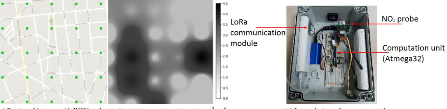
(a) Region of interest with WSN nodes (b) Simulation errors’ variance ((µg)2/m6) of June, 2008
(c) Internal view of our sensor nodes
Fig. 1: WSN nodes locations, simulation errors corresponding to the district of La-part-dieu, Lyon, France during June, 2008 and an internal view of our sensor nodes.
A. Dataset
We perform the evaluation of our proposal on monthly pollution data corresponding to the 2008 Nitrogen Dioxide (NO2) concentrations in the Lyon district of La-Part-Dieu,
which is the heart of the Lyon City. This pollution data set has been generated by an enhanced atmospheric dispersion simulator called SIRANE [6], which is designed for urban areas and takes into account the impact of street canyons on pollution dispersion. The dataset has been provided by LMFA, which is a research lab specialized in fluid mechanics in the Lyon city, France.
The region of interest has a spatial resolution of 100 meters and is depicted in Fig. 1a with a set of 25 pollution sensors. We calculate the correlation coefficients Wpq using
an exponential decay function. That is, the correlation between points decreases exponentially with the euclidean distance.
We recall that the main input of our scheduling approach is the variance of the errors of the physical model. In this evaluation part, we assume that the errors of the model are linearly correlated with its concentrations. Let γ express the linear relationship between the model concentrations and the model errors. Thus, we first calculate the variance of the concentrations of the physical model based on the pollution maps and then we multiply these variances by γ2 to get the variance of the physical model errors. We calculate the γ parameter by evaluating the linear regression between the concentrations of the dataset of the physical model and the real data of the few monitoring stations which are already deployed in the Lyon city. For illustration purposes, we depict in Fig. 1b the variance map of the physical model errors corresponding to the month of June.
In order to consider a real scheduling scenario, we use the characteristics of an air pollution monitoring system that we developed in our lab (see Fig. 1c). The energy consumption required for sensing, transmission and reception per month as well as the default simulation parameters are depicted in TABLE II. In all the results presented in this section, we used the Cplex MILP solver to optimally solve our scheduling
model while using a PC with Intel Xeon E5649 processor under Linux.
Parameter Notation Value Number of sensors N 25 Communication range of sensor nodes R 500m Sensing error stp 0.5(µg)2/m6 Battery capacity E Ip 518.4 kJ Sensing monthly energy consumption E Stp 129.6 kJ Transmission monthly energy consumption ETpt 129.6 kJ Reception monthly energy consumption E Rt
p 51.84 kJ
TABLE II: Default values of main simulation parameters.
B. Proof of concept
In order to provide a proof of concept of our scheduling approach, we run our model while considering the default simulation parameters and we set coverage requirements to 1( µg)2/m6. We get an optimal network lifetime equal to 3 months as depicted in Fig. 2 (from left to right: January, February and March). We notice that the number of active sensors is different depending on the time period. In fact, the correction of the air pollution physical model requires more nodes depending on the variability of air pollution within each time period. We also notice that some nodes are active in more than one time period. Indeed, according to the default simulation values, the battery capacity allows sensor nodes to run up to two months without stop.
We also evaluate the assimilation error provided by the sensor nodes that are active during the months of January, February and March. Results are depicted in the same Fig. 2. We notice that the assimilation error never exceeds the coverage requirement set to1( µg)2/m6thanks to the coverage constraints of our optimization model.
C. Impact of coverage requirements on the network lifetime In this simulation scenario, we investigate the impact of coverage requirements on the maximization of the network lifetime. We consider 3 different values of the battery capacity and we vary the the coverage requirements from0.5( µg)2/m6
Fig. 2: Proof-of-concept: optimal WSN activity scheduling and the corresponding estimation errors’ variance (( µg)2/m6) while considering coverage requirements equal to 1( µg)2/m6. Active sensors are depicted in blue squares.
to 2.5( µg)2/m6. The obtained results are depicted in Fig. 3. We notice that the higher the assimilation error threshold, the higher the network lifetime. This is expected since with less coverage requirements, less sensors are activated during each time period allowing us to get multiple subsets of sensor nodes capable, each of which, of ensuring coverage and connectivity constraints.
In terms of battery capacity impact, as expected the higher the initial amount of energy per node, the largest the network lifetime. However, doubling the battery capacity does not always involve twice lifetime as shown in the curves when the assimilation error threshold is equal to 1.4 ( µg)2/m6. Indeed, this depends on the variability of pollution within each time period and which may require different number of active nodes.
Fig. 3: Impact of battery capacity. D. Impact of sensing frequency on the network lifetime
We now evaluate the impact of sensing quality on the network lifetime. We consider two scenarios while varying the sensing frequency of nodes: in the first case, sensors analyze the quality of the air without stop whereas in the second case, sensing is performed during only 30 seconds every minute. It is worth mentioning that in the latter, the node is kept active during the non sensing 30 seconds which is necessary for the air pollution electrochemical sensing probes. Reducing the sensing frequency impacts both energy consumption and the
correction of the physical model. In order to understand how the the sensing frequency impacts the network lifetime, we depict in Fig. 4 the obtained results while varying the coverage requirements. Results show that first, coverage requirements cannot be met with low sensing frequency for an assimilation error threshold that is less than 1( µg)2/m6. Indeed, with
low sensing frequency, the sensing error of nodes goes up from0.5( µg)2/m6 to1( µg)2/m6. Moreover, we still get lower
network lifetime when using low sensing frequency. However, as the assimilation error threshold of the physical model goes up, we tend to get the same results for both sensing techniques because the sensing errors become tolerable with respect to the assimilation process.
Fig. 4: Impact of sensing quality.
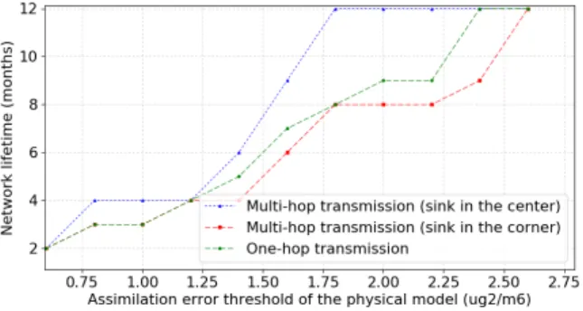
E. Impact of transmission power on the network lifetime In the last simulation scenario, we analyze the impact of transmission power on the network lifetime. Increasing the transmission power allows us to get larger transmission range but at the cost of energy consumption. We consider three different cases: i) high transmission power (our LoRa powered nodes with 20dbm transmission power) allowing us to get one-hop communication to the sink node (communication range equal to 500m); ii) low transmission power (14 dbm) with a communication range equal to 200 in non line of sight while considering the sink node in the corner of the map; and finally iii) low transmission power with the sink node
in the center. Results are depicted in Fig. 4 and show that despite the multi-hop communication, low transmission power leads to better network lifetime compared to high transmission power. However, this is not always the case as the results also show that one-hop communication is preferable over multi-hop communication if the sink node is not well positioned (in the corner rather than in the center of the map for instance).
Fig. 5: Impact of transmission power. VIII. CONCLUSION
In this paper, we focus on extending the lifetime of the network by scheduling the sensing activity of sensors. Our objective is to decide which sensors should be turned off in order to let the network operate longer while ensuring the ap-plication requirements. We design a mathematical model and a heuristic algorithm that we use to determine which sensors should be turned off based on the collected data. Related works in the literature focused only on two main applications: target detection and spatiotemporal field construction. Our work is different in the sense that we consider a different and a new challenging application which is the correction of physical models. We use the data assimilation technique to provide a mathematical formulation to the locations where data is not needed for the correction of the physical model. We apply linearization techniques and linear relaxation to get solvable optimization models. Finally, we evaluate our proposal on an air pollution dataset from the Lyon city, France and provide engineering insights on the optimal scheduling of air pollution sensors.
As future work, we plan to perform simulations on different environmental applications while studying the quality of our approach depending on the nature of the physical model. Another perspective of our work would be to analyze the impact of weather conditions on the longevity of the electronic components of sensor nodes.
ACKNOWLEDGMENT
We would like to thank the anonymous reviewers for their comments and feedback. This work has been supported by Mi-tacs, Canada and the "LABEX IMU" (ANR-10-LABX-0088) of Université de Lyon, within the program "Investissements d’Avenir" (ANR-11-IDEX-0007) operated by the French Na-tional Research Agency (ANR).
REFERENCES
[1] J. Yick, B. Mukherjee, and D. Ghosal, “Wireless sensor network survey,” Computer networks, vol. 52, no. 12, pp. 2292–2330, 2008.
[2] A. Boubrima, W. Bechkit, and H. Rivano, “Error-bounded air quality mapping using wireless sensor networks,” in Local Computer Networks (LCN), 2016 IEEE 41st Conference on. IEEE, 2016, pp. 380–388. [3] ——, “Optimal wsn deployment models for air pollution monitoring,”
IEEE Transactions on Wireless Communications, vol. 16, no. 5, pp. 2723–2735, 2017.
[4] W. Du, Z. Xing, M. Li, B. He, L. H. C. Chua, and H. Miao, “Sensor placement and measurement of wind for water quality studies in urban reservoirs,” ACM Transactions on Sensor Networks (TOSN), vol. 11, no. 3, p. 41, 2015.
[5] V. Roy, A. Simonetto, and G. Leus, “Spatio-temporal sensor manage-ment for environmanage-mental field estimation,” Signal Processing, vol. 128, pp. 369–381, 2016.
[6] L. Soulhac, P. Salizzoni, P. Mejean, D. Didier, and I. Rios, “The model sirane for atmospheric urban pollutant dispersion; part II, validation of the model on a real case study,” Atmospheric Environment, vol. 49, pp. 320–337, 2012.
[7] A. Tilloy, V. Mallet, D. Poulet, C. Pesin, and F. Brocheton, “Blue-based no2 data assimilation at urban scale,” Journal of Geophysical Research: Atmospheres, vol. 118, no. 4, pp. 2031–2040, 2013.
[8] H. Yetgin, K. T. K. Cheung, M. El-Hajjar, and L. H. Hanzo, “A survey of network lifetime maximization techniques in wireless sensor networks,” IEEE Communications Surveys & Tutorials, vol. 19, no. 2, pp. 828–854. [9] S. Biswas, R. Das, and P. Chatterjee, “Energy-efficient connected target coverage in multi-hop wireless sensor networks,” in Industry Interactive Innovations in Science, Engineering and Technology. Springer, 2018, pp. 411–421.
[10] F. Tashtarian, M. H. Y. Moghaddam, K. Sohraby, and S. Effati, “On maximizing the lifetime of wireless sensor networks in event-driven applications with mobile sinks,” IEEE Transactions on Vehicular Tech-nology, vol. 64, no. 7, pp. 3177–3189, 2015.
[11] M. Hu, J. Zhang, Y. Yu, H. S.-H. Chung, Y.-L. Li, Y.-H. Shi, and X.-N. Luo, “Hybrid genetic algorithm using a forward encoding scheme for lifetime maximization of wireless sensor networks,” IEEE transactions on evolutionary computation, vol. 14, no. 5, pp. 766–781, 2010. [12] P. G. Liaskovitis and C. Schurgers, “Leveraging redundancy in
sampling-interpolation applications for sensor networks: A spectral approach,” ACM Transactions on Sensor Networks (TOSN), vol. 7, no. 2, p. 12, 2010.
[13] Y. Lin, J. Zhang, H. S.-H. Chung, W. H. Ip, Y. Li, and Y.-H. Shi, “An ant colony optimization approach for maximizing the lifetime of heterogeneous wireless sensor networks,” IEEE Transactions on Systems, Man, and Cybernetics, Part C (Applications and Reviews), vol. 42, no. 3, pp. 408–420, 2012.
[14] J. Du, K. Wang, H. Liu, and D. Guo, “Maximizing the lifetime of k-discrete barrier coverage using mobile sensors,” IEEE Sensors Journal, vol. 13, no. 12, pp. 4690–4701, 2013.
[15] M. E. Keskin, ˙I. K. Altınel, N. Aras, and C. Ersoy, “Wireless sensor network lifetime maximization by optimal sensor deployment, activity scheduling, data routing and sink mobility,” Ad Hoc Networks, vol. 17, pp. 18–36, 2014.
[16] S. Mini, S. K. Udgata, and S. L. Sabat, “Sensor deployment and scheduling for target coverage problem in wireless sensor networks,” IEEE Sensors Journal, vol. 14, no. 3, pp. 636–644, 2014.
[17] C.-P. Chen, S. C. Mukhopadhyay, C.-L. Chuang, M.-Y. Liu, and J.-A. Jiang, “Efficient coverage and connectivity preservation with load balance for wireless sensor networks,” IEEE sensors journal, vol. 15, no. 1, pp. 48–62, 2015.
[18] X. Deng, B. Wang, W. Liu, and L. T. Yang, “Sensor scheduling for multi-modal confident information coverage in sensor networks.” IEEE Trans. Parallel Distrib. Syst., vol. 26, no. 3, pp. 902–913, 2015. [19] Z. Lu, W. W. Li, and M. Pan, “Maximum lifetime scheduling for
target coverage and data collection in wireless sensor networks,” IEEE Transactions on vehicular technology, vol. 64, no. 2, pp. 714–727, 2015. [20] M. Asch, M. Bocquet, and M. Nodet, Data assimilation: methods,
algorithms, and applications. SIAM, 2016.
[21] W. Revelle, “An introduction to psychometric theory with applications in r,” 2009.