Cognitive Information Processing

(1)

XVII. COGNITIVE INFORMATION PROCESSING

Academic and Research Staff

Prof. M. Eden Prof. T. S. Huang Prof. F. F. Lee Prof. C. Levinthal Prof. S. J. Mason J. Allen G. B. Anderson T. P. Barnwell III B. A. Blesser A. J. Citron P. C. Economopoulos A. Gabrielian C. Grauling R. E. Greenwood E. G. Guttmann R. V. Harris III D. W. Hartman H. P. Hartmann A. B. Hayes G. R. Kalan

Prof. K. Ramalingasarma

Prof. W. F. Schreiber

Prof. D. E. Troxel

Dr. W. L. Black

Dr. K. R. Ingham

Dr. P. A. Kolers

Graduate Students

R. W. Kinsley, Jr.

A. N. Kramer

W-H. Lee

C-N.

Lu

J. I. Makhoul

G. P. Marston III

O. R. Mitchell, Jr.

S. L. Pendergast

D. R. Pepperberg

G. F. Pfister

R. S.

Pindyck

W. R. Pope, Jr.

D. S.

Prerau

G. M. Robbins

Dr. O. J. Tretiak C. L. Fontaine P. H. Grassmannt E. R. Jensen J. E. Green R. A. Schaffzin K. B. Seifert C. L. Seitz D. Sheena D. R. Spencer W. W. Stallings P. L. Stamm R. M. Strong C. R. Tegnelia Alice A. Walenda G. A. Walpert J. W. Wilcox J. J. Wolf J. W. Woods I. T. Young

A. CUBIC CORNERS$

One structure that comes frequently before our eyes in this urban world is the cubic

corner. This is simply any corner of a cube, of a desk or box, or in general 3 planes

meeting at right angles. The simplest line drawing of a cubic corner consists of a point

with 3 radiating straight lines of indefinite length. For easy reference, such a drawing

will be called a 3-star.

The fact is that 3-stars tend to look like cubic corners. That is, the visual

sys-tem tends to interpret them as the projections of cubic corners.

This is not so

under all conditions. Not only the 3-star itself, but any larger scene in which a

3-star is imbedded may influence its interpretation.

Moreover, it is likely that

our urban experience contributes to this propensity;

the Watusi might not join the

trend at all.

*This work was supported principally by the National Institutes of Health (Grants

1 PO1 GM-14940-01 and 1 PO1 GM-15006-01), and in part by the Joint Services

Elec-tronics Programs (U. S. Army, U. S. Navy, and U. S. Air Force) under Contract

DA 28-043-AMC-02536(E).

tOn leave from Siemens A.G., Erlangen, Germany.

IThis work was supported in part by Project MAC, an M. I. T. research program

Office of Naval Research Contract Nonr-4102-(01).

(2)

(XVII. COGNITIVE INFORMATION PROCESSING)

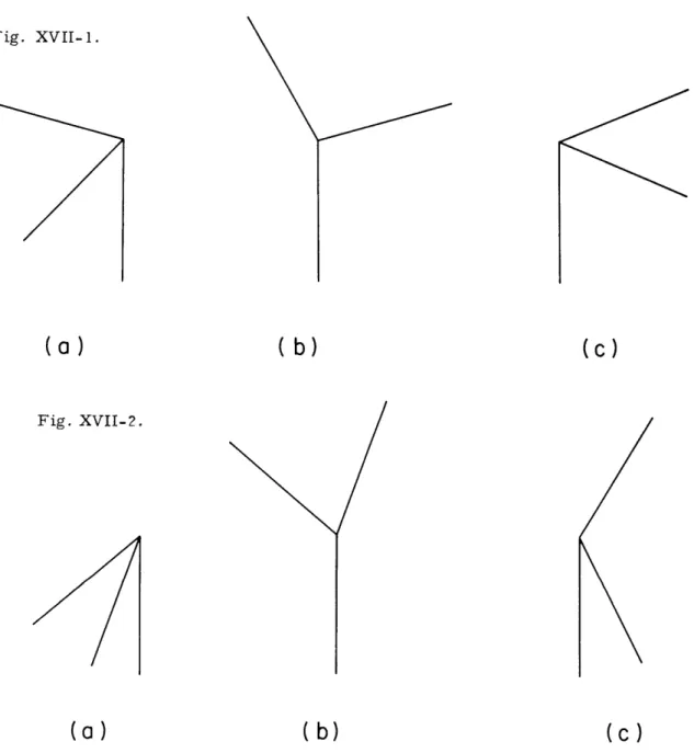
In Fig. XVII-1 there are some 3-stars that look like cubic corners. In Fig. XVII-2 there are some that do not.

Fig. XVII-1.

(a)

Fig. XVII-2.

(a)

(b)

(c)

(b)

(c)

Figure XVII-3 exemplifies how context can influence interpretation. The 3-star of Fig. XVII-3a appears in Fig. XVII-3b and XVII-3c in places indicated by stars (*).

Figure XVII-3a may look like a cubic corner to the reader, as it does to the author. At any rate, Fig. XVII-3b contains the 3-star in a context that certainly makes it appear cubic. _{Figure XVII-3c, on the other hand, contains the 3-star in such a way that it} looks like a wedge of not too wide an angle. _{The circular arc on the left of Fig. XVII-3c} suggests a wedge of cheese.

(3)

Fig. XVII-3.

(a)

(b)

(c)

One might suspect that the interpretation of a 3-star is just a matter of context and has nothing to do with the 3-star itself. In Fig. XVII-3b, a drawing looking like a rectangu-lar solid was constructed about the 3-star by putting the sides of the 3-star into parallel-ograms and completing the figure. Try this procedure with the 3-star in Fig. XVII-4a; the results are hardly analogous. Figure XVII-4b does not look rectangular at all.

Fig. XVII-4

(4)

The orientation as well as the context of a 3-star can influence its interpretation. The 3-star in Fig. XVII-5a can readily be seen as a cubic corner. Yet in Fig. XVII-5b where the figure is rotated 900, the smallest angle no longer appears to be right, but rather acute. _{Figure XVII-5c speculates on one of the common scenes in our} experi-ence which might lie behind such an orientation dependency.

Three-stars are most likely Fig. XVII-5. _{to look like cubic corners when}

one of the rays points directly downward. Most cubic corners that one sees on buildings, boxes,

and such things are oriented with their planes perpendicular or

parallel to the ground, and con-sequently have one vertical edge.

(a)

(b)

_{Probably a down-pointing ray in}

a 3-star invokes these

experi-ences.

Still there is the question, How does the structure of the 3-star itself influence its inter-pretation? One can determine mathematically which 3-stars can be perspective projections of

cubic corners. We shall illustrate this a bit later. The diagrams

already presented show that the

visual system will not accept that certain 3-stars look like cubic corners. The questions then are,

(C) How critical is our visual system?

Does one reject 3-stars that could be cubic corners? Does one accept 3-stars as cubic corners when they could not possibly represent them geometrically? How well does the visual system align itself with the requirements of geometry and perspective ?

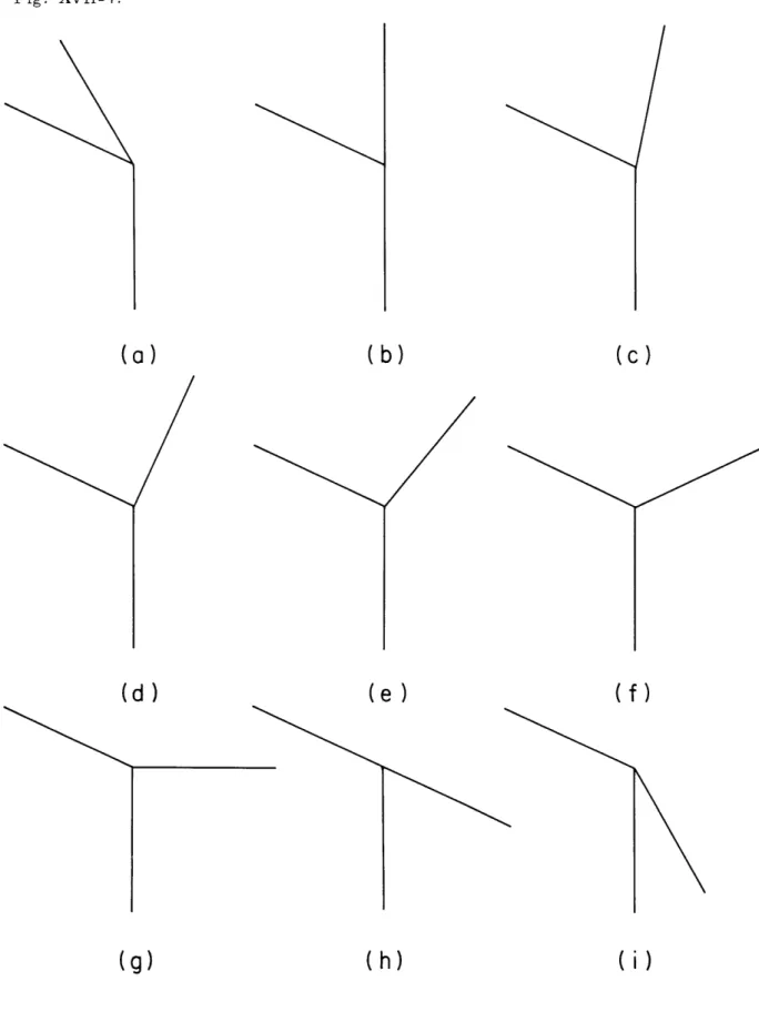
Figures XVII-6 and XVII-7 contain two series of 3-stars for the judgment of the eye. All have rays pointing straight down to enhance the seeing of cubic corners. In the series of Fig. XVII-6 the 3-stars b through d and j through 1 are acceptable to the eye as

cubic corners (if in doubt, construct parallelograms around them), and these cubic cor-ners have two faces in view. In Fig. XVII-7 only d through g are seen as cubic corcor-ners,

(5)

Fig. XVII-6.

(a)

(d)

(g)

(b)

(e)

(c)

(f)

(h)

(i)

(k)

(I)

(m)

(6)

Fig. XVII-7.

(a)

(d)

(g)

(b)

(e)

(h)

(c)

(f)

( i )

(7)

The empirical generalization suggested by Fig. XVII-6 and other sketches is: A 3-star is acceptable to the visual system as a 2-faced cubic cor-ner if and only if it contains 2 angles less than or equal to 900, whose

sum is greater than or equal to 90 .

The generalization suggested by Fig. XVII-7 and other sketches is:

A 3-star can appear to be a 3-faced cubic corner only if all 3 angles are greater than or equal to 90 .

Now that there is some empirically derived notion of what the visual system inter-prets as a cubic corner, the problem is to determine which 3-stars are perspective views of cubic corners.

At first thought, it would seem necessary to calculate an arbitrary perspective pro-jection of an arbitrarily oriented cubic corner. This is not the case for two reasons. In the first place, the eye is assumed to be focused on the vertex of the cubic corner; in the second place, only the angles between the projected rays, and not their length in projection, are of concern. Under these conditions, perspective can be ignored and the projection of a cubic corner in X Y Z space will simply be its orthogonal projection on the X Y plane.

Suppose that some 3-star has angles between its rays a, b, c, and also that the rays are represented by unit vectors P, Q, R in the X Y plane. The question is, Are there 3 vectors in X Y Z space which are mutually orthogonal and project, respectively, to P,Q,R?

Since projection is accomplished merely by dropping the Z component, any 3 such vectors must have the form:

P + pZ Q + qZ R + rZ, (1)

where Z is the unit vector in the Z direction, p, q, r scalars. Requiring mutual orthog-onality is requiring that the dot products of these vectors in pairs be zero. Using dis-tributivity of the dot product and remembering that P, Q, R are unit vectors yields (2), and similarly for the pairs Q, R and R, P.

(P+pZ) - (Q+qZ) = 0 = P -

Q

+ pq = cos a + pq = 0. (2) This produces three equations:

pq = -cos a qr = -cos b rp = -cos c (3)

Solving for p, q, r, we obtain

(cos a)(cos c) (cos a)(cos b) (cos c)(cos b)

p= - q= - r=

(cos b) (cos c) (cos a)

(8)

Hence solutions exist and are given by these formulas, provided that (cos a), (cos b),

(cos c) f 0, and (so that the numbers under the radicals will be positive) either one or

three of cos a, cos b, cos c are negative.

The solutions in (4) have singularities where cos a, cos b, or cos c = 0; that is,

where a, b, or c = 900 or 2700. To what do these singularities correspond in the

situa-tion under study ?

If there is only one 90 or 270

angle, this represents the situation in which one ray

of a cubic corner is pointed directly away from or toward the observer, and hence only

2 edges (not a 3-star) are visible.

If there are two 90 angles, the solutions to (4) contain the indeterminate form 0/0.

This situation occurs when one plane of the cubic corner is oriented edgewise to the

viewer.

This is the only case when a 3-star that is a projection of a cubic corner can

contain a right angle.

Any other combination is impossible, since a + b + c = 1800.

Aside from the singularities, What does the requirement that either one or three of

cos a, cos b, cos c be negative represent? If, say, only cos c is negative, this implies

that a is less than 90 , b is less than 900, and a + b is greater than 90 . If all three,

cos a, cos b, and cos c, are negative, this implies that a, b, c, are all greater than 90

0 The rules derived mathematically agree with the rules derived empirically, except

for the 3-stars containing one right angle!

To rephrase the conclusion:

Given a 3-star in favorable conditions of orientation and context and not containing

one right angle, the visual system will accept that 3-star as a cubic corner if and only

if it could in geometric fact be a projection of a cubic corner.

Fig. XVII-8.

A 3-star that does have one right angle cannot be the geometric projection of

a cubic corner. Yet the visual system will often accept such a 3-star as a cubic

cor-ner (Fig. XVII-8).

(9)

B. SURFACE RECONSTRUCTION FROM CONTOUR SAMPLES: SOME COMPUTER SIMULATION RESULTS

Briefly, the problem is the following: Given the constant elevation contours of some surface, how should one reconstruct the surface? This problem has been viewed as a statistical estimation problem, and the equation governing the estimate has been derived previously.

For simulation purposes, the two-dimensional random field was scanned, thereby producing a random process. Level-crossing times, together with the corresponding levels, were used as inputs to a reconstruction algorithm.

The computer was used to study how the reconstruction scheme would behave with such information. Only the most elementary reconstruction formula for the scanned field was implemented. The source process that was used was a black and white snap-shot. The statistical processing of the snapshot was compared with one that had been quantized to the same levels and with one in which straight lines joined crossings.

1. Basic Reconstruction Formula

By assuming that the scanned field is Gaussian and by ignoring all of the inequality information except at the estimation point, the equation2

B z exp(--z 2) dz x(t) = m(t) + 0-(t)

f

B

exp(- z2) dz

may be applied. The integral in the denominator is computationally difficult to evaluate. Also, the role played by that quotient of integrals is to supply a number between A and B, that is, the center of gravity of the Gaussian density between A and B. In this case,

it is justifiable to use the Cauchy density instead of the Gaussian density. If A and B are both much greater or less than zero, however, the Cauchy approximation to the cen-ter of gravity is very bad, but the estimation formula still does not suffer. The actual

estimation function that was used was

i a(t) In [(l+B2 )/ (+A2)]

m(t) + -1 , AB

>

-1

2 tan-i [(B-A) /(1+AB)]

x(t) =

(1)

1 a(t) in[(1+B2) /(1+A2)]

m(t) +

-

, AB < -l,

-w + tan [(B-A) /(1+AB)]

(10)

determined so that

2

exp z2 dz = dx

-2

-2x

+ K

The symbols are defined as follows: x is the estimate at point t; the conditional mean is m(t); and the standard deviation is o(t). Both of these are conditioned upon the wave-form passing through the levels at the corresponding crossing times. The two func-tions a(t) and P(t) bound the original waveform: a(t)

<

x(t) < p(t). These bounding functions arise because level crossings have been detected.

For each particular estimation point t, only the sample values at the two neighboring crossing times are used. Denote crossing times t , and the corresponding levels x . Let R(s, t) be the autocorrelation function for x(t). The mean of x(t) restricted to pass through xj at t.j and xj+l at tj+ is

m(t) = a.x. + a. xI

j

j j+1

j+l'

where the aj, aj+1 satisfy

R(t, t ) = ajR(tj,tj) + aj+₁R(tj+l'tj) R(t, tj+1)

= ajR(tj+ 1' tj) + aj+ 1R(tj+ 1' tj+1)

Also, the process is assumed to be stationary so that a normalized autocorrelation

2 2

function may be usefully defined: p(T) = R(T)/- . When _{2 is written without an} argu-ment "(t)", it will denote the variance of the stationary, unrestricted process x(t). Also,

for notational convenience, set X = t - t = = tj+ t t, T - tj. The solution for aj and aj+1 is

a = [p(X)-p(T)p(T)]/[1-p2(T)

aj+₁ = [p(X)p(T)-p(T)]/[1-p 2

_(T)].

The variance of x(t), restricted just as the mean was, is

2 (t) = a 2[1-ajp(X)-aj+1P( )].

2. Level-Crossing Processing

It is assumed that the input waveform has been sampled periodically in time at a rate fast enough so that the original may be reconstructed adequately by straight lines through the samples. _{The level-crossing processing has two steps: the crossing times and}

(11)

corresponding levels are extracted from the input waveform by assuming that straight

lines join the samples, and the input waveform is reconstructed by applying the

inter-polation equation.2 The reconstructed waveform is represented at the original periodic

sample times.

Some of the crossing times were eliminated because they included no time at which

the waveform was to be reconstructed.

Perhaps this would be best clarified by an

4

Fig. XVII-9. Detection of the level crossings

of the sampled waveform.

23

2 t₁3 t₃ t4 4

example.

In Fig. XVII-9 the input waveform is shown in its sampled form.

To extract

the crossing times, one may picture straight lines joining the samples. Between t = 3

and t

=

4 there are 3 level crossings. In this example, the crossing times t

2

and t

3

are

ignored.

In general, between any two samples of the input waveform, if there are any

crossings, only the rightmost crossing is retained.

To reconstruct the waveform from these crossing times, each adjacent pair is taken

successively.

Then, for each such pair t , t+1, the interpolation formula is evaluated

at all points in the half-open interval [tj, tj+l)

at which the input was sampled.

3. Processing of the Snapshot

The snapshot was quantized into 1024 brightness levels, and was sampled on a 256X

256 grid. It was also necessary to know the autocorrelation function of the process. For

the particular photograph used here, autocorrelation function has been estimated.3 The

values for the mean,

ii,

and the standard deviation, a-, where

j=403

and a-=234. The

normal-ized autocorrelation

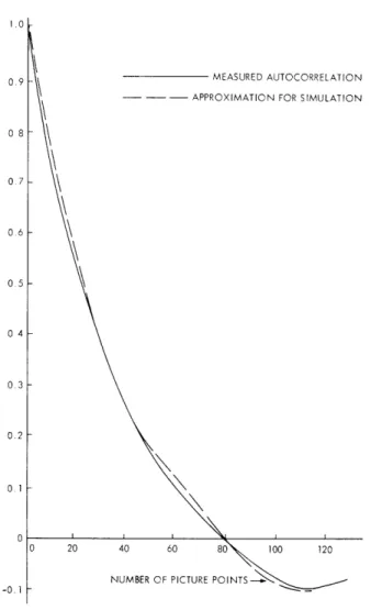
p(T)

is shown in Fig. XVII-10.

Also shown is a polynomial

approx-imation to p(T) that was used in the reconstruction.

The approximation of p(T) must be

done with some care. For example, the formula for -2(t) gives a negative result if

(12)

10-0 9 MEASURED AUTOCORRELATION

- - APPROXIMATION FOR SIMULATION

08 0.7 0.6 0.5 04 0.3 0.2 01 0 0 20 40 60 80 100 120

NUMBER OF PICTURE

POINTS---0. 1

Fig. XVII-10. Normalized autocorrelation functions.

p(T) = 1 - ST2, no matter what value of s is used and no matter how small the crossing interval, T, may be.2

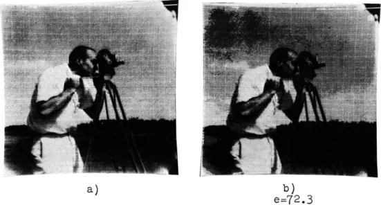
The results of reconstructing the photograph from crossing-time information may be seen in Figs. XVII-11 and XVII-12. In either of these figures (a) is the original, (b) is a quantized version, (c) is a reconstruction using straight lines between crossings, and (d) is the statistical reconstruction. The difference in processing between Figs. XVII-11 and XVII-12 is that 8 equispaced levels are used in Fig. XVII-11, and

16 equispaced levels in Fig. XVII-12. The value of e shown in each case is the square

root of the mean-square error per picture point: 256 256

e2 =

j=1

i=1

(13)

a)

b)

e=72.3

-O-c) d)

e=47 3

e=34.1

N=11670

Fig. XVII-11.

(a) Original.

(b) Quantized to 3 bits.

(c) Straight-line reconstruction.

(d) Statistical reconstruction.

(14)

a)

b)

e=37.7

c)

d)

e=22.9

e=16.0

N=18679

_N=18679

Fig. XVII-12. (a) Original.

(b) Quantized to 4 bits.

(c) Straight-line reconstruction.

(d) Statistical reconstruction.

(15)

Fig. XVII-13.

Level-crossing points.

(a) 8 levels, equispaced in brightness.

(b) 16 levels, equispaced in brightness.

(16)

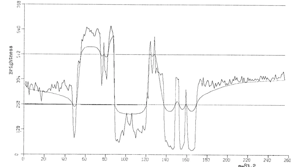
Fig. XVII-14. Reconstruction of the middle scan line - 4 levels.

=-83.2

2

(17)

(

V

_

_______________I II I A.r - - I I II I I I b s I 2

0

20 q

0

60

80

00

120 1410

160

180

Fig. XVII-15. Reconstruction of the middle scan line - 8 levels.

CO LO C.. CD to Cl] 4) bO pr (c h0

200

0

240 e=34.1

260

22 V\4dW"

vt

---4 1 1 - - - -ld_~ ~1 ALAn- _v

(18)

'

I

U

0

120

1

40 16F

1I0

O

20 q0

6U

S0

L00

120 16U

6O

]80

2002

Fig. XVII-16. _{Reconstruction of the middle scan line}- 32 levels.

C rI)1 T) C~ cu- CI-CC)J

0 11fL

§1-___--

_1ka

r

220 e=9.70

I

21

260

__ __L____~_________ __ ___~__

_~_ _~__

I __

___~_I___

I~

___~ _ _

_____~_~___

__f_ ___~

__

I _ _I~

_I_ ~

I_

_~I___

_____~

__I_ ~I___

___ ~I

I_ _~_

___ _I~_ I__

_____~_~_~_~ ~I ~1~1_

~__II

____ I_~__

----~- ______ ~-

-

--__

(19)

Also, the value of N is given under (d) and (e). N is the total number of crossings detected. In Fig. XVII-11d the top eighth of the photograph is a constant. This was an input-output error with the magnetic tape, and is unrelated to any reconstruction pro-cedure.

In Fig. XVII-13, the points at which the crossing times were detected are shown. Part (a) shows the crossings points for 8 levels, and (b) shows them for 16 levels. There was a total of 65, 536 = (256)2 grid points. With 8 levels 11, 670 crossings were detected, and with 16 levels 18, 679 crossings were detected.

Besides having the smallest error, the statistically processed photograph has less-ened the effect of the spurious contours and abrupt changes in brightness, which is so apparent in the quantized photograph. The fact that the photograph was processed in a horizontal direction is not apparent in Fig. XVII-12d, but is noticeable in Fig. XVII-lld. A disturbing feature of this statistical reconstruction is that the snapshots appear to have

less contrast, but this is because the highest the reconstructed waveform may reach is approximately midway between the second highest and highest levels. Similarly, it never goes lower than the middle of the lowest and next to lowest levels.

In the straight-line interpolation scheme the same crossing times were used as those in the statistical scheme.

The straight-line scheme performs very poorly. It is apparent that the processing was done horizontally. Also, there are abrupt, artificial changes in brightness. Clearly, one could improve upon this simple interpolation scheme. The point in trying it was just to compare this simple interpolation scheme with the statistical one. Another point brought out by the straight-line interpolation is that the mean-square error is not a complete measure for goodness of fit. Even though the error was comparable to the error for the statistical interpolation, the appearance of the statistically reconstructed picture is of higher quality than the picture reconstructed by straight-line interpolation.

Shown in Figs. XVII-14, XVII-15, and XVII-16 are graphs of the statistical recon-struction of the middle scan line of the photograph. The number of levels are shown on each graph, and the original input is superimposed on the reconstructed version. They may be distinguished because the original has an apparent low-magnitude, high-frequency portion on the extreme right.

One aspect of this statistical reconstruction is demonstrated by these graphs. Very fast large-magnitude jumps in the process are always found, but the low-magnitude higher frequencies, in general, are missed.

G. M. Robbins References

1. G. M. Robbins, "Surface Reconstruction from Contour Samples," Quarterly Prog-ress Report No. 87, Research Laboratory of Electronics, M. I. T. , October 15, 1967,

(20)

2. G. M. Robbins, _{"Surface Reconstruction from Contour Samples," S.M. Thesis,} M. I. T. , February 1968; see especially Equation (1), Sec. 4. 1.

(21)

C. FIELD SHADING AND NOISE IN THE SCAD SCANNER

1. Approximation Procedure

It is hoped that a scanner will give a constant signal when scanning a uniform field. This is not likely to happen; the signal will be biased by the deterministic nonuniformi-ties in a scanner (shading), and perturbed by random noise.

In a flying-spot scanner such as SCAD1 the deterministic distortion of the signal can be characterized fairly simply. The measured signal is a linear function of the trans-mittance, so that nonuniformities of the light transmission path can be compensated by measuring the signal produced by the scanner from a clear field, and by scaling the signal from a transparency by the reciprocal of the clear-field characteristic.

Two problems arise when one wishes to estimate the shading or the deterministic clear-field variation. The signal from the scanner is corrupted by noise, so that, to make such an estimate, one must perform the calculation in terms of a stochastic model. The analysis might be done by repeatedly scanning a clear field, and by finding

histo-grams of values at each point in the field. Because of practical limitations, this was not feasible; hence, our analysis was done from single recordings of the signal. The second difficulty arises when one wishes to use the data for correcting the signal. Unless the data on the shading are summarized by a few parameters, it may not be feasible to perform the correction.

We decided to model the clear-field variation by a linear composition of several functions that are easy to compute and are likely to fit the shading pattern well. If f(I, J) is the clear-field signal recorded over the raster 1 < I < IM, 1 J

<

JM, and fA(I, J) is a function of the form, then

u

fA(I, J, al . . an) = aif(I J).

i= 1

The coefficients a ... an are chosen to minimize the difference:

IM JM

e(al. .

.an)

= _{(f(I,J) - fA(I,J, al..}_._an))Z I=l J=l

We define the approximation error as

Min a e(an) 1/2

Mina1. .. a n aThe IM * JM

(22)

random noise, and shading that the fA function could not fit. We take the expression

IM JM-1

1/2

ed 1(f(I, J)-f(I, J+1))2

2 IM(JM-1) I=l J=

as a measure of the rms white noise in the signal. The quantity

2 1/2

e

=

(e

2a-ed 2

is an estimate of the variation in the signal that is neither white nor fitted by fA' 2. Physical Sources of the Variation

The optical system used in SCAD is shown in Fig. XVII-17. The feedback signal modulates the grid drive to the cathode-ray tube in an attempt to keep the signal from the feedback PMT constant. The beam splitter that sends a signal to the feedback PMT is placed behind the imaging lens, so that the feedback system collects light over the

FEEDBACK PMT

]

RED SIGNALBLUE SIGNAL CONDENSER

CATHODE- /

RAY TUBE _{Fig. XVII-17. SCAD scanner optics}

GREEN SIGNAL (top view).

IMAGING \

LENS BEAM CONDENSER DICHROIC

SPLITTER DICHROIC MIRRORS

TRANSPARENCY

same solid angle as the transparency sensing path. One surface of this mirror is metallized to reflect approximately 30% of the light, and the other surface has an antireflection coating. The light transmitted by the transparency is split into color components by interference filters.

The principal sources of signal shading are the imperfections in the feedback system, and differences between the feedback and signal optical paths. The reflectance from a mirror depends on the incidence angle, and this angle varies when the scanner explores the transparency. The angle of incidence on the beam-splitting mirror varies over

450 ± 130, and the angle of incidence on the dichroic mirrors is 450 ± 60. The cone

of rays from the lens, when the lens is at maximum aperture, is ± 60. The reflectance-wavelength characteristics of the dichroic mirror depends on the angle of incidence and, since the light from the CRT is not white, this introduces both color and intensity variation. One may also expect variations because of artifacts such as dust or smudges

(23)

on the mirrors and condenser lenses.

One expects white noise from the amplifiers and the shot effect in the photo-multiplier tubes, as well as 60 Hz pickup. With the light levels and integration times encountered in this system, these effects should be very small. Phosphor noise, or light variations because of the granularity of the phosphor, are expected to be white, and although the light feedback is supposed to cancel this, this cancellation is not perfect.

3. Results and Discussion

Clear-field signals from the three color channels were recorded on magnetic tape from a raster, 108 samples wide and 173 samples high. The placement of this raster relative to the field of view of the scanner is shown in Fig. XVII-18. The signal was quantized to 6 bits.

2.5

cm-AREA USED

FOR THE

TEST-SCANNER

FIELD OF

VIEW

T

E

+

O

₁₎

10( - 5cm

I

5 cm

Fig. XVII-18. Area used in the field of view test.

The clear-field signals were processed according to the procedure described above. The functions used in the expansion are listed in Table XVII-1. The coefficients obtained from the analysis are given in Table XVII-2. These coefficients have been scaled so that the amplitude of the constant function, fl', is unity.

The variation in the clear-field signal seems to be described almost completely by the expansion in terms of the approximation functions and the white noise. The term eu that measures the departure from this model is ~1%0, and this seems to be

small enough to cause no concern under most conditions. We expect this term to be due to hum and errors in the approximation, and since there is a significant variation in eu between the three fields and we expect the hum to be the constant, this variation is

(24)

Table XVII-1. Expansion functions.

f (I, J) = 1

f 2(I, J) = cos (((I-1)/(IM-1) -. 5) *T)

f 3(I, J) = cos (((J-1)/(JM-1)-. 5) r r)

f4(I, J) = sin (((I-1)/(IM-1) - . 5) * )

f5(I, J) = sin (((J-1)/(JM-1) - . 5) * r)

f₆(I, J) = f4 f5

Table XVII-2. Field shading and noise coefficients.

Field al a2 a3 a4 a5 a6 e ed e

Red 1. 00 -.0190 .0086 .1011 -.0071 .0009 .0271 .0263 .0075

Green 1. 00 -.0107 .0529 .0089 .0076 .0072 .0230 .0213 .0086

Blue 1. 00 -.0406 -.0230 -.0943 .0221 .0075 .0276 .0244 .0129

probably due to approximation errors.

The white noise, estimated by e_{d ,} is much larger than is tolerable, and an effort will be made to reduce it. Its source has not been established, although it is definite that only a small part of it is caused by shot or quantization noise.

O. J. Tretiak References

1. 0. J. Tretiak, "Scanner Display (SCAD)," Quarterly Progress Report No. 83, Research Laboratory of Electronics, M. I. T., October 15, 1966, pp. 129-142.

(25)

D. BIOLOGICAL IMAGE PROCESSING - AUTOMATED LEUKOCYTE RECOGNITION

Enormous amounts of time are expended in medical laboratories every day in the routine examination of smears prepared from human peripheral blood. The reason for making this examination is twofold: to possibly locate abnormal or pathological cells; and, more commonly, to perform a differential leukocyte (white cell) count. The very repetitive nature of this second test leads us to ask if it could be automated. That is, could we find an algorithm that could perform the differential count more efficiently and accurately than it is now being done. This is the task of automated leukocyte recognition.

1. Background

Suspended in the plasma (liquid) of mammals are 3 distinct types of cells: red cor-puscles (erythrocytes), colorless corcor-puscles (white blood cells or leukocytes), and blood platelets. The leukocytes, which number between 5000 and 9000 cells per cubic millimeter of blood, are considered true cells, that is, they possess both a well-defined nucleus and a cytoplasm. The cells seen in dry smears are quite different from the same cells seen in living preparations. In the dry smears the normally spherical cells are flattened to large thin disks.

Leukocytes may be subdivided into two different categories: (a) nongranular leuko-cytes, and (b) granular leukocytes. Extensive examination of stained, dry smears has shown that these two categories may be further subdivided into the 5 types of leukocytes found in normal blood samples.

A. Nongranular Leukocytes 1. Lymphocytes 2. Monocytes B. Granular Leukocytes 1. Eosinophils 2. Neutrophils 3. Basophils

When a blood smear, stained with Wright's stain, is examined under an oil-immersion microscope at 1000X magnification, the 5 different types of leukocytes may be differen-tiated according to the morphological (shape) and spectral (color) information summa-rized in Table XVII-3. Pictures of the different types of leukocytes are shown in Fig. XVII-19.

(26)

Table XVII- 3. Morphological and spectral characteristics of leukocytes.

Cell Type Population Diameter Cytoplasm Nucleus Granules

( ) (

Color Amount Color Shape Amount Amount

Clear

Lymphocyte 25-33 7-12 Light 10-30% Purple Round 70-90% Few

Blue

Monocyte 2-6 13-20 Grayish 50% Light Indented 50% Few

Blue Purple

Neutrophil 60-70 10-12 Pink to 50% Reddish Segmented 50% Many

Lilac Purple

Eosinophil 1-4 10-14 Red 60-70% Dark Two-Lobed 30-40% Many

Stippling Blue

Basophil .25-.5 10-12 Blue 50% Purple Elongated 50% Many

Pale

Red Cell 4-6 X 106 4-6 Orange 100% None - 0% None

(27)

(XVII.

COGNITIVE INFORMATION PROCESSING)

NEUTROPHIL

LYMPHOCYTE

EOSINOPHIL

BASOPHIL

MONOCYTE

Fig. XVII-19.

Normal human leukocytes (1000X).

2. Optical Image Processing

Using Kodachrome II-A film, we photo-micrographed a standard blood smear stained

with Wright's blood stain. The field of view was approximately 70

±

X 50 [1 and contained

50 red cells, 1 lymphocyte, and 1 neutrophil. The color transparency was scanned

through SCAD, a flying-spot color scanner, and the resulting digital data were recorded

on magnetic tape.

The resolution of the entire system at this point was limited by the

resolving power of the microscope:

(28)

R 0. 61 X n. a.

For a center wavelength Xc = 0. 55 p., and the n. a. of the microscope objective (n. a. = 1. 32) yields a resolution limit of approximately 0. 25

p.

For leukocytes this is roughly the size of the granules in the cytoplasm.

The three one-color pictures generated by SCAD were read into the Project Mac 7094 computer, and a program was developed to produce a multi-grey level picture on the off-line printer. By using an overprinting technique described by Mendelsohn and modified for the CTSS character set, a picture was produced that reduced the original 64 grey-level picture (corresponding to 6-bit quantization) to 17 distinct grey levels. A photograph of the "red picture" (the original color transparency viewed through a red

Table XVII-4. Grey-level overprint codes.

Output Input Over- Print

Level Levels Symbol

1 0-2

MR

2 3-5 RM 3 6-8 IW 4 9-11 WW 5 12-15 WX 6 16-19 XX 7 20-23 XV 8 24-27 VV

9 28-31

V/

10 32-35

//

11 36-39 /, 12 40-43 W 13 44-47 X 14 48-51 V 15 52-55

/

16 56-59 17 60-63

(29)

(XVII. COGNITIVE INFORMATION PROCESSING)

filter) is shown in Fig. XVII-20.

A list of the grey-level overprint codes is given in

Table XVII-4.

Examination of Fig. XVII-20 immediately reveals a major problem.

Because of a

nonuniformity in the scanner, the background illumination varies across

the picture.

(30)

The result of this is that contrast is reduced in many portions of the picture, and in some places it is almost impossible to separate the cells from background. This prob-lem was solved by the following analysis. Let a pure black point be denoted by the num-ber 0 and a pure white point by 63. Now, for the sake of simplicity, assume that the nonuniformity occurs in a purely horizontal direction, that is, along a scan line. If there were no distortion in the scanning illumination and we recorded a perfectly clear field, then we would get a brightness versus position curve as shown in Fig. XVII-21la. Because of the nonuniformity, however, plus our observation that in Fig. XVII-20 we are in general able to distinguish the cells from background, we may conclude that the background illumination is a slowly varying function of position. We shall call this phe-nomenon "tilt" after the simulated picture of the nonuniformity in Fig. XVII-21b.

BRIGHTNESS BRIGHTNESS

63- 63

-45 45-

-L POSITION L POSITION

(a) (b)

Fig. XVII-21. Effect of scanner nonuniformity.

Although the details of the derivation will not be given here, it is an easy matter to show that the effect of the two-dimensional tilt B(x, y) on any picture brightness distri-bution f(x, y) is to change the distridistri-bution to

f'(x,y) = B(x,y) f(x,y).

Since B(x,y) is slowly varying as compared with f(x, y), we may approximate it by the lowest frequency terms in a two-dimensional Fourier series expansion of f'(x,y) when f(x, y) is a constant (that is, when a clear field is recorded). Thus we have B(x, y) = 1 + B₁sin(blx) ₊ B2 c o s (b2x) +B 3 s i n (b3y) + B4 c o s (b4y) + B5 s i n (b5x) s i n (b6y).

By dividing the recorded picture f'(x,y) by the calculated B(x,y), pictures are obtained that have good contrast and uniform background illumination.

3. Pattern Recognition

Before a leukocyte can be identified it must first be located in the 70

p

X 50 p. field of view. Since there are approximately 650 red cells for every leukocyte, the problem of overlapping leukocytes can be ignored. Thus if we consider the picture to be

(31)

represented by its 18, 500 points, every point can be classified as belonging to one of

three types: (a) background points; (b) red cell points; (c) leukocyte points.

In order to speed computation, the background points are immediately eliminated

from further consideration by the following technique.

For each of the three one-color

pictures a histogram is computed of the first-order brightness distribution. A sample

histogram is shown in Fig. XVII-22a.

The histogram is then smoothed as shown in

Fig. XVII-22b, and the relative maxima and minima are located on the smoothed

histo-gram.

By analysis of several pictures, we have found that the second minimum from

the left represents a clipping level to separate background points from red and white

cell points. The results of this type of clipping are shown in Fig. XVII-23.

To separate the remaining points in the picture into the two classes

-

red cell and

leukocyte

-

the "classical" approach of pattern recognition was used.

In this approach

an appropriate feature or set of features is determined and then, by using an appropriate

decision function on the resulting feature space, unknown objects may be classified by

measurement of these features.

The feature used in our case is the two-dimensional

chromaticity per point. Briefly, chromaticity may be defined as follows.

Consider the

spectral distribution SX of a point in the color picture. By passing the light from this

point through the two dichroic mirrors of the SCAD system, the three digitally recorded

numbers (red, green, and blue) are given by the expressions

R =

C

1(X) SX dX

G =

C

2

() S

k

dX

B = C₃(X) SX dX,

where the CK(k) are the spectral transmission functions of the respective light paths.

The chromaticity pair (r, g) per point is computed by taking the ratios

R

r

_R+G+B

G

g=R + G + B'

By computing chromaticity statistics over a set of known and identified points and then

using a maximum-likelihood decision function to classify unknown points, we have had

reasonable success in separating red cell points from leukocyte points (Fig. XVII-24).

(32)

-ajnlOTd

,Pal,,

@141 JO

UOTlnqTilSTP SS@UjLj2Taq

I@PTO-IS.ITJ (U)

'ZZ-IIAX

'2Tq

t9 xxxxxxxxx 29 xxxxxxx 9 xxxxxxxx L9 xxxxxxx 09 xxxxxxx 6 xxxxxxx 9 xxxxxx L xxxxx 9 xxxxx xxxxxx t xxxxxxx 2 xxxxxxx Z xxxxxxxx L xxxxxxxx 0 xxxxxxxxxxxxxx 6t xxxxxxxxxxxxxxxxxxxx 8 xxxxxxxxxxxxxxxxxxxxx L xxxxxxxxxxxxxxxxxxxxx 9t xxxxxxxxxxxxxxxxxxxxxx t XXXXXYXXYXXXYXXXXXX tt xxxxxxxxxxxxxxxxxxxxx E YXYXYYYYYYYXXYYXY 2 xxxxxxxxxxxxxxxxx Lt xxxxxxxxxxxxxx ot xxxxxxxxxxxxxxxx 62 xxxxxxxxxxxxxxxxxx G xxxxxxxxxxxxxxxxxxxxxxxx L xxxxxxxxxxxxxxxxxxxxxxxxxx 92 YxXxxxxxxxxxxxxxxxxxxxxxxxxx 92 xxxxxxxxxxxxxxxxxxx xxxxxxxxxxxxxxxxxxxxxxxxxxxx H xxxxxxxxxxxxxxxxxxxxxXXXXXXXXXXXXXXYXX H xxxxxxxxxxxx L xxxxxxxxxxxxxxWlyxXxxxxx H xxxxxxxxxxxxxxxxxxxxxxx 6 xxxxxxxxxxxxxxxxxxxxxxxx 8 XXXXXXXXXXXXXXXXXXXXYxxxx ze XXXXYXXXXXXXXXXXYXXYYxxxx 9 xxxxxxxxxxxxxxxxxxxxxxxxxxx XXXYXXXXXXXXXXXXXXXYXxxxxxxxxxxxxx tz XYXXXXXX xxxxxxxxxxxxxxxxxxxxxxXYXXXXXX H x xxxxxxxxxxxxxxxxxxxxxxxxxxxxxxxxxxxxx e XXXXXXXXXXXXXYXXXYXXXxxxxxxxxxxxxxxxxxxxxxx Le xxxxxx XXXXXXXXXXXXXXXXXXXXXYxxxxxxxxxxxxxxxxxxxxxxx oz 6L XXXXXXXXIAIYXYXXXXXXXXXXXXXXYXXXXXXXXYXXXXXXXXYXXY-YXXXXXXXXXXXX SL A;kxxxxxxxxxx XXXXXXXXXXXXXYXXXXXXXXxxxxxxxxxxxxxxxxxxxxxxxxxxxxxxxxxx LL XXX>"X XXXXXXXYXYXXXXXYXXXYXYxxxxxxxxxxxxxxxxxxxxxxXYXXXXXXXXYXX 9L XXXXXXXXXXXXXXXXXYXXXxxxxxxxxxxxxxxxxxxxxxxxxxxxxxxxxxxxxx 9L XXXXXXXXXYXXXXXXXXXXXXXXXXXXXXXXYXXXXXXXXXXxxxx xxxxxxxxxxxxxxxxxxxxxXXXXYXXXXXXXXXXXXXXXXXxxxxxxxxxx xxxxxxxxxxxxxxxxxxxxxxxxxxxxxxxxxxxxxxx eL xxxxxxxxxxxxxxxxxxxxxxxxxxxx LL xxxxxxxxxxxxxxxxxx OL xxxxxxxxxxxxxx 6 xxxxxxxxx 8 xxxxxxxxxxxxxx L xxxxxxxxxxxxxx 9 xxxxxxxxxxxx xxxxxxx xxxxx xxxxxxxxxxx z XXXXXXXYXXXXXXXXXXXXXx L XXXXXXXXXXXXXYXXXYXYXxxxxxxxxxxxxxxxxxxxxxxxxxxxxxxxxXXXXXXXXXXYXXXX 0 eL = 10RAS HOV3 M ]AIVA VMVdXVA

(33)

-aan~od "pa

oq

jo uoijnqTijsip

poqloouiS

(q)

'ZZ-IJAX

T

'A9 Y9 09 X\XXXMXXXXXA) K XX~xxx)XXXXXX) G XXXXXXXX'xx))\X lot X\XXXX)xxxxXXXXX rxf \VXXXAXXXXXXXXX t? XXXXXXXXXN XX\X)XXXX i XXXXXXXXXXXmxxXXXXXXX t \\) XXXXXX~xx)xxxx)xxxxx XAXXX0xxAxxxxxxxx)xxxx L \AK\NN\AXXXX0MXXXXXX 'f A AAXXXXAAKAXX\) xx K 'x x A XX\A >AX x xX'AX i XXXXXXXXXX XXN)XXXX XXX0 2 X\X)XXXXXXXXXXXXXX XX XxXX) XKXAX\ x XXXX )XXX)XXXXXXXx tZ XXX XX'', XXXXXXXXX XXX>XXXX\X) X?'AX x XXXXXXXXXXXXXX'' XXXXXXXXX X XX 'XXXX IA X XXXA X X /, XXAX X, X ,/ X\ X X \XXX XX X XXX XXXXX XX X X X X X X X 0,X\ X>X X X X X XXX XX XXXXAXXXX AX XX X,

X

XX xx X XX X 0XX XXXXXX XX XX xXxXX XX x)\XA, /AX X L1 XXXXXXX) XX XXXXXXXX Ax XX A XX X/, YXxX, L \XXXXXXXXXXXXX\XXXXXXxxxxXx\/ XXXXXX L X'AXX\X\X~~xXXXXXXXXXXXX), tXXXXXXXXX A XAXX~~~ KKXX)AXXXXXX)XX X X XX \XY/,\X XKXA/X/ X 1 ,XXXX\'A1X\X)AXx xx 'A! AX\XX),x xX xxx\ XAAX)XX X XK/ LI X A// "~ l yX\X XAAAAXA XX

X XX

XXXXX X\ X X XXAXXX X X X "\)axXX\ XX NXA X !XAXAAYA\XXX/~~~~~~~~ ,,'\!X)) -,I)XXAAXXXXXXX)XAA A)

~ ~ ~

~

: A'\A'AAX AA)A V\AXX)AA)XX\XAAi A>\ K, MY -I

(34)

(35)

4:-~~p--I-

,-Fig. XVII-24.

"Red" picture with leukocyte points identified.

.. .. ...

P~~~e~~"eu;~~ '" :4

(36)

4. Summary

We have recently recorded and are in the process of analyzing 6 more full-color

blood-smear pictures to obtain refined chromaticity and shape statistics.

Using these additional pictures and the investigation of specific morphological

prop-erties of leukocytes and their nuclei, we expect to complete our task of leukocyte

dif-ferentiation.

I. T. Young

References

1. I. Davidsohn and B. Wells, Clinical Diagnosis by Laboratory Methods (W. B.

Saunders Company, London, 13th edition, 1965), Chaps.

1, 2,

and 4.

2. M. L. Mendelsohn and B. Perry, "Picture Generation with a Standard Line Printer,"

Communs. ACM, Vol. 7, No. 5, pp. 311-313, May 1964.

3. M. L. Mendelsohn and J. Prewitt, "Analysis of Cell Images," Ann. N. Y. Acad.

Sci. 128, pp. 1035-1053, January 1966.

4. O. J. Tretiak, "Scanner Display

-

SCAD," Quarterly Progress Report No. 83,

Research Laboratory of Electronics, M. I. T.

,

October 15, 1966, pp. 129-142.

5. G. S. Sebestyen, Decision Making Processes in Pattern Recognition (Macmillan

(37)

(XVII. COGNITIVE INFORMATION PROCESSING)

E. DIFFERENTIAL LEUKOCYTE ANALYSIS BY OPTICAL METHODS

We are investigating the possibility of differentiating leukocytes from the charac-teristics of their scattered light, rather than by examining their image. It is well known that if an object is illuminated with collimated light along the axis of the optical system, the spatial Fourier transform of the object will be seen in the back focal plane of the

system. We hope to use this property in an arrangement as shown in Fig. XVII-25. Our primary reason for considering this system is that the magnitude of the Fourier transform, that is, the scattered light in the back focal plane, does not depend (in

prin-ciple) on the distance between the cell and the lens, nor on the position of the cell relative to the axis of the optical system. Therefore the cell need not be either registered

OBJECT f FOURIER

- C~ TRANSFORM

PLANE

ELECTROMAGNETIC LENS

WAVE

Fig. XVII-25.

Fourier transform property of

lenses.

CAMERA VIEW

MAGNIFYING LENS (LEITZ LICHTEINSTELLUPE)

FOCAL PLANE WITH

FOCAL PLANE OPAQUE TOP

(ON GLASS-PLATE) OBJECTIVE (LEITZ 12.5/0.3)

CELL -- MASK (50 pO)

PARALLEL LIGHT

LAMP (CONDENSER REMOVED)

]

MIRROR

Fig. XVII-26. Microscope changed to perform

Fourier transform of leukocytes.

or in focus.

Thus this technique can be applied in a system in which the cells flow

in a liquid past some sort of sensing element. It seems obvious that a system like this

would be much easier to automate than one in which the cells must be prepared on a

slide and scanned in focus.

(38)

Another possibility is that since index of refraction variations scatter light, it may

be possible, in the system under discussion, to differentiate unstained cells.

The signal that can be recorded in the system

under consideration is essentially the squared

ampli-tude of the Fourier transform.

Since this is the

transform of the autocorrelation function, we see

that the final signal will contain much less

informa-tion than the original image. The major leukocyte

types differ with respect to the following attributes:

size, shape or nucleus, and granules in the

cyto-plasm.

The size differences will affect the spatial

Fou-+5

-1

rier transform at approximately 10

m

, the

nucleus shape at approximately 3 X 10

+ 5

m

- ,

and

(a)

the nuclear granules at 3

X

106 m

.

The system shown in Fig. XVII-26 was used for

our initial experiments. Since the diameter of a single

cell is only approximately 10 l, we expected that

some effort would be needed to overcome noise

prob-lems, that is, the background of the Fourier

trans-form produced by light scattering inside the lens,

by diffraction by its margins, and by general

reflec-tion inside the system. The experimental

arrange-ment consisted of a microscope changed in the

following manner:

(i) We removed the condenser

(b)

to illuminate the picture with parallel light.

(ii)

We replaced the ocular by a magnifying lens,

Fig. XVII-27.

_{which enlarged the focal plane of the objective,}

(a) Background of the Fourier

in which the Fourier transform of the cells occurs.

transform system.

(b) Signals of two leukocytes.

(iii) We placed an aperture of approximately 50

±

diameter behind the cell to keep the illuminating

beam as small as possible in order to reduce the background. (iv) We mounted a small

opaque stop in the focal point of the objective to absorb the DC component of the Fourier

spectrum. With this arrangement signals of single leukocytes could be detected.

Fig-ure XVII-27a shows the background of the system, and Fig. XVII-27b shows the

back-ground and the additional signal produced by two unstained leukocytes.

The system does not seem to produce very accurate Fourier spectra, and before

trying some different optical systems we have decided to study some promising

configu-rations by simulating them with a computer.

(39)

(XVII. COGNITIVE INFORMATION PROCESSING)

F. READING MACHINE FOR THE BLIND

Members of our group are working on experimental reading machine systems with the eventual aim of providing sensory aids for the blind. The present experimental sys-tem was not intended as a prototype of a practical reading aid but rather as a real-time

research facility for experimental investigation of human information requirements and human learning capabilities upon which prototype designs must be based. The experi-mental system development has involved, and will facilitate, research on print scanning, character recognition, control by a blind reader, and auditory and tactile displays.

The reading machine system diagram is shown in Fig. XVII-28. The PDP-1 com-puter is operated in a time-sharing mode by a remote console and the data link provides the necessary communication and control links to

CONTROL

CARRIAGE the

equipment

in our

laboratory.

The

audio

out-put of the data link is used when spelled speech is selected as the output of the reading machine. SCANNERDISPLAY

CONTROL _{Other output mechanisms now available are a} typewriter and a Braille embosser. The

scan-DATA A UD1O

LINK AUDIO ner control is a moderately complex digital sys-tem incorporating approximately 1000 integrated PDP- TYPEWRITER circuits. It effectively extends the instruction

set of the PDP-1 and permits overlapping of Fig. XVII-28. computations and local processing operations. Reading machine system diagram. The scanner control also incorporates a visual

display of the scanner output. The carriage con-trol is an open-loop digital servo that permits a page of text to be moved in horizontal

and vertical directions at approximately 200 steps per second, where there are approx-imately 4 steps per letter.

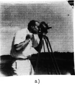
The opaque scanner is shown in Fig. XVII-29. For the cathode-ray tube we used a Tektronix oscilloscope mounted on end. The dot of light from the cathode-ray tube is imaged through a single lens onto the paper, and the diffuse reflected light is collected by means of 2 photomultiplier tubes. When the scanner controller wishes to determine the blackness of a particular location on the page, it supplies the proper xy signals to the oscilloscope, unblanks the beam, and the output of the photomultiplier tubes is inte-grated for a fixed time. If this inteinte-grated output exceeds a threshold voltage, then the point is said to be white.

In Fig. XVII-30 the over-all sequence of operation is indicated. The initialization of the program also includes selecting the proper initial position for the carriage. The first line of text is then acquired, by using a special directive provided by the scanner

(40)

CARRIAGE PINITIALIZE PROGRAM

MECHANISM PAPER

LENS/ ACQUIRE LINE

FILTER

S ICOMPUTE CONSTANTS

ACQUIRE CHARACTER CARRIAGE

HAS YES RETURN

LINE ENDED?

CARRIAGE

NO TRACE CONTOUR

cRT

I GENERATE SIGNATURE

FIND SYMBOL

UNBLANK _{SPELL SYMBOL} _CARRIAGE

Fig. XVII-29. Opaque scanner. Fig. XVII-30. PRM-1 flow chart.

control. This is where the size of the type font is determined and various constants are computed to aid in the recognition of punctuation and in the rejection of miscella-neous specks. After this, the first character is acquired, with a carriage motion if it is necessary, and it is determined whether or not the line has ended. If not, the exter-nal contour of the letter is traced, again by using another special directive provided by the scanner control, and a characteristic number or signature is generated. After the signature has been generated, a table of previously encountered signatures is searched for a match. If a match is found, a symbol is retrieved and an auditory output is initi-ated, after which the next character is acquired and the process repeats.

The process for acquiring a line of text uses a horizontal histogram that is com-puted by determining the total number of black points at each y level and normalizing the curve. A simple threshold procedure is used to determine the two interior lines,

and the remaining lines are computed from these two lines. As successive letters are traced, these y lines are updated, and the carriage moved vertically, if necessary, to track text that is not exactly aligned horizontally.

The next two operations are the acquisition scan and the contour trace. The verti-cal limits of the acquisition scan are the two exterior lines as determined from the horizontal histogram. The scan starts at the lower left, traces a vertical line, and then indexes to the right by one and repeats the vertical line until it encounters a black point. At this point the contour trace instruction is given, and if the exterior of the

(41)

black area is very small, it is considered to be a speck and ignored.

If it is another

size classification, it is deemed punctuation, and a special routine is used to determine

which of the punctuation marks it is.

Figure XVII-31 contains a clear presentation of a character contour and also gives

an indication of the resolution of the scanner. If the circumference of the black area is

large enough that it is deemed a character, a

sig-nature is computed by the method indicated in

Fig. XVII-32. The starting point is always at the

westernmost point. Local extrema are determined

for the horizontal and vertical directions if the

excursions along the contour are greater than

one-quarter of the letter height or width.

That is, for

example, an x maximum is not denoted unless one

had to travel east for at least one-quarter of the

let-ter width and then west for one-quarlet-ter of the letlet-ter

Fig. XVII-31. Capital

'S'

contour.

width. With this scheme, minor features of the

let-ter such as the droop in the upper left part of the

a do not introduce extraneous extrema. The sequence of extrema can be coded with one

bit per extremum if the starting point is assumed to be an x minimum and the contour

trace is clockwise. In addition to this sequence of extrema, the quadrant in which it

was determined

is stored for such extrema.

01 XMIN II These binary sequences, together with a small

amount of information concerning the aspect ratio

XMAX YMAX

of the letter and its position relative to the y lines

found by the histogram procedure, comprise the

--- -- signature.

START In order for characters

to

be recognized, the

S-/4

particular signature must have been encountered

HEIGHT

XMAX

previously; that is,

the machine must have been

SWIDTH 0 previously trained by a sighted operator. To enable

TART=I

the sighted operator to recognize the letters, a

Y =0

CODE WORD: I I I 1 0 visual

display is

made.

When the machine is

COORDINATE WORD: 00 01 01 II 10 00

unsuccessful in the search for a match for a

par-Fig. XVII-32.

ticular signature, it can effectively ask the trainer

Determination of extrema.

what the character is.

Given this information, it

can thus add to its experience. There is a certain

amount of noise involved in the determination of black and white, and the presence of

this noise actually simplifies the training procedure, as it appears that successive

tracings of the same a have variations similar to tracings of different a's. Thus with

(42)

the carriage control disabled, one can lock on to a particular letter and build a reper-toire of signatures for that particular letter.

In several accuracy tests, the results have been about the same, with an error rate of approximately one-third of one per cent. Training has been virtually completed on two fonts and others are in process. Punctuation marks are recognized and are spelled

out to minimize the storage space required for the speech output. The spelled-speech output consists of letters that have been digitized and artificially shortened so that their duration is under 100 msec. This puts a limit of 120 wpm as the maximum output rate. The present machine, however, alternates the speech output with the rec-ognition process, and the average speed is approximately 80 wpm.