Design of the gas-puff imaging diagnostic for Wendelstein 7-X

Design of the Gas-Puff Imaging Diagnostic for

Wendelstein 7-X

by

Kevin Tang

Submitted to the Department of Nuclear Science and Engineering

in partial fulfillment of the requirements for the degree of

Bachelor of Science in Nuclear Science and Engineering

at the

MASSACHUSETTS INSTITUTE OF TECHNOLOGY

June 2019

© Massachusetts Institute of Technology 2019. All rights reserved.

Author . . . .

Department of Nuclear Science and Engineering

May 16, 2019

Certified by. . . .

James L. Terry

Principal Research Scientist

Thesis Supervisor

Accepted by . . . .

Michael P. Short

Chairman, Department Committee for Undergraduate Students

Design of the Gas-Puff Imaging Diagnostic for Wendelstein

7-X

by

Kevin Tang

Submitted to the Department of Nuclear Science and Engineering

on May 16, 2019, in partial fulfillment of the

requirements for the degree of

Bachelor of Science in Nuclear Science and Engineering

Abstract

Stellarators, being not as well-studied as tokamaks, have plenty of interesting physics

to examine, as investigations of stellarators as a viable configuration for future power

plants continue. One of these aspects is boundary turbulence in the plasma, as the

magnetic configuration in stellarators is different from that in tokamaks and thus

provides different plasma behavior. To study this turbulence, we are designing a

“gas-puff imaging” diagnostic to install onto the Max Planck Institute of Plasma

Physics’s Wendelstein 7-X (W7-X), which is currently the world’s most advanced and

largest stellarator. This diagnostic employs a fast-camera to observe a localized puff

of gas as it interacts with the boundary plasma near the last closed flux surface of the

plasma. The diagnostic consists of a fast-camera component, a light-collection

com-ponent, a “gas-puff” component with valves to inject controlled amounts of gas, and

a component for valve control and data collection purposes. This thesis documents

some of the aspects of the design of the diagnostic and its components for W7-X.

Thesis Supervisor: James L. Terry

Acknowledgments

I’d like to thank James L. Terry, Seung-Gyou Baek, and Sean Ballinger for their

mentorship and assistance over the past two years.

Contents

1

Introduction

15

2

Background

17

2.1 Differences between Tokamaks and Stellarators . . . .

17

2.2 Phantom Fast-Camera Diagnostic Overview . . . .

19

2.3 Gas-Puff Imaging Diagnostic Standard . . . .

21

3

Design Methodology and Results

23

3.1 Port Selection . . . .

23

3.2 Fast-Camera Subsystem . . . .

24

3.2.1 Simulations for the Phantom v710 Optical Setup . . . .

26

3.2.2 Simulations for the APDCAM-10G Optical Setup . . . .

27

3.3 Gas-Puff Valve Subsystem . . . .

29

3.4 Valve Control and Data Collection Subsystem . . . .

31

3.4.1 Red Pitaya Field-Programmable Gate Array . . . .

31

3.4.2 Python Graphical User Interface . . . .

34

3.5 Heat Loading Simulations . . . .

36

3.5.1 Heat Load Analysis of the Gas Puff Nozzle . . . .

36

3.5.2 Heat Load Analysis of the Immersion Tube . . . .

38

4

Summary

41

B Tables

55

C Code and Scripts

59

C.1 block_design.tcl . . . .

59

C.2 config.yml . . . .

64

C.3 extension_connector.xdc . . . .

66

C.4 GPI_2.hpp . . . .

67

C.5 GPI_2.py . . . .

75

C.6 DataCollect.vhd . . . .

79

C.7 outputs.vhd . . . .

81

C.8 GPI_Valve_GUI.py . . . .

87

List of Figures

2-1 Schematics of magnet and plasma configurations in (a) tokamaks and

(b) stellarators [1]. . . .

18

2-2 Bench view of the Phantom diagnostic within its soft iron box. The

Phantom camera, seen on the top rail, is optically connected to a

turn-ing mirror, then to a beamsplitter, and finally to a lens coupled with

the fiber optic bundle. . . .

19

2-3 (Left) View of the MIT fast-camera with divertor panels labeled and a

cross-section of plasma flux surfaces superimposed. (Right) A

single-frame snapshot of plasma emission, showing the typical enhanced

emis-sion along the divertor strike-line. . . .

20

2-4 Overview of the mechanics for gas-puff imaging. The neutral gas is

puffed perpendicular to the local magnetic field, and the line emissions

are then observed by the fast-camera pointing parallel to the magnetic

field at the point of interaction to observe boundary turbulence [2]. .

21

3-1 Fusion Instruments APDCAM-10G (left) and the microlens array (right).

This will be the camera we will be using for the GPI diagnostic, with

a 4x8 microlens array coupled to the camera for near 100% photon

detection efficiency. . . .

25

3-2 (Top) Optical system for the case where the Phantom v710 is chosen for

the GPI. Photons from the plasma in the top right are reflected by the

angled turning mirror, then channeled through the vacuum window,

and finally through the series of lenses to the focus of the camera on

the far left. (Bottom) Zoomed in view of the system of lenses and

objective lens pictured in the far left of the overview. . . .

26

3-3 Optical system for the case where the APDCAM-10G is chosen for the

GPI. Photons from the plasma in the top right are reflected by the

angled turning mirror, then channeled through the vacuum window,

and through three lenses to focus onto the camera. . . .

28

3-4 CAD rendering of the gas-puff valve subsystem with all of the

compo-nents in place on the mounting plate. . . .

29

3-5 General schematic of the Red Pitaya STEMlab 125-14 components.

The Red Pitaya has on-board processor and FPGA, along with RAM

and network connectivity on top of customizable pins in the extension

connectors [3]. . . .

32

3-6 Detailed pin descriptions of the extension connectors [4]. . . .

32

3-7 General overview of the FPGA design layout. . . .

33

3-8 Overview of the Python GUI. . . .

35

3-9 COMSOL analysis of the gas puff nozzle with the back panel cooled.

36

3-10 COMSOL analysis of an idealized situation for the gas puff nozzle with

a larger fraction of the mounting bracket cooled to 30°C. . . .

37

3-11 COMSOL analysis of the optical system with one set of cooling pipes.

Port AEE50 can be seen on the left, while the 880°C plasma sheet can

be seen on the right. . . .

38

3-12 COMSOL analysis of the optical system with two sets of cooling pipes

flanking the vacuum window to cool the length of the tube as much as

possible and therefore the window as well. . . .

39

4-1 Overview of all of the components of the GPI diagnostic in place at

their respective port locations. . . .

41

4-2 Overview of the entire GPI diagnostic from a different angle than in

Fig. 4-1. The sightline intersecting with the injected gas can be clearly

seen. . . .

42

A-1 Plasma cross section at the toroidal angle of the gas puff nozzle at

port AEK50. Prominent plasma features such as the LCFS in blue

and plasma islands in red are also shown. . . .

46

A-2 Various details for general characteristics of the Zemax simulated

Phan-tom v710 optical system. . . .

47

A-3 Spot diagram for the Phantom v710 simulation. The image on the top

left is that of the on-axis object, whereas the other two correspond to

off-axis objects. We can thus see that the focused image spot is at best

0.4 mm in size and at worst 1.4 mm, which is acceptable for the 4x4

mm detector. . . .

48

A-4 Geometric encircled energy plot for the Phantom v710 simulation. The

on-axis case reaches 100% enclosed photon energy at around 0.34 mm,

while the off-axis cases reach about 90% at that point. . . .

49

A-5 Various details for general characteristics of the Zemax simulated

APDCAM-10G optical system. . . .

50

A-6 Spot diagram for the APDCAM-10G simulation. The image on the

top left is that of the on-axis object, whereas the other two correspond

to off-axis objects. We can thus see that the focused image spot is at

best 0.1 mm in size and at worst 0.2 mm, which is well acceptable for

the 23.4x39 mm detector. . . .

51

A-7 Geometric encircled energy plot for the APDCAM-10G simulation.

The on-axis case reaches 100% enclosed photon energy at around 0.055

mm, while the off-axis cases reach about 90% at that point. . . .

52

A-8 Overview of the FPGA design in Vivado Design Suite. . . .

53

List of Tables

B.1 Detailed specification of the various distances and parameters

neces-sary to generate the optical system for the Phantom v710 case. The

radius column refers to the radius of curvature of the optical elements,

the thickness the distance separation between two faces of those

ele-ments, and the semi-diameter their radial size, all of which are in mm.

The materials were selected to have the same optical qualities as those

that would be actually used and blank materials indicate air. These

values have been optimized within Zemax to provide the best focus at

the detection plane. The overall distance between the gas puff and the

detection plane is approximately 2800 mm. . . .

56

B.2 Detailed specification of the various distances and parameters

neces-sary to generate the optical system for the APDCAM-10G case. The

columns are defined the same way as those in Table B.1. These values

have been optimized within Zemax to provide the best focus at the

detection plane. The overall distance between the gas puff and the

detection plane is also approximately 2800 mm. . . .

57

Chapter 1

Introduction

Since the 1960s, research with regards to harnessing nuclear fusion to generate energy

has taken off and branched into multiple subfields. Within the magnetic confinement

fusion subfield, the leading reactor design candidate for realizing a fusion nuclear

power plant is the tokamak, since historically it has provided the best results in

approaching net energy generation. However, recent manufacturing innovations and

work with another type of magnetic configuration, the stellarator, have shown that

it may be another promising candidate for energy generation purposes, as it is able

to contain the fusion plasma in steady-state operation.

In the field of fusion research, while tokamaks have been widely studied,

stellara-tors are relatively novel; thus there are many aspects of stellarator physics that require

study. One particular issue that magnetic confinement fusion faces is plasma

turbu-lence, which carries heat and particles out of the confined plasma. As such, plasma

turbulence and its behavior must be mitigated in order to successfully implement a

viable fusion power plant in the future.

Wendelstein 7-X (W7-X), of the Max Planck Institute for Plasma Physics (IPP)

in Greifswald, Germany, is currently the world’s largest and most advanced

stel-larator now undergoing experimental campaigns with hydrogen plasmas, with the

long-term goal of attaining steady-state continuous operation for thirty minutes. An

MIT Plasma Science and Fusion Center (PSFC) group, consisting of Principal

Re-search Scientist James L. Terry, ReRe-search Scientist Seung-Gyou Baek, PhD Student

Sean Ballinger, and me, is currently designing a gas-puff imaging (GPI) diagnostic

to install onto W7-X in late 2019 or early 2020, in time for W7-X’s second operation

phase in 2021. Although GPI diagnostics have been previously installed onto

toka-maks, the GPI diagnostic being designed for installation onto W7-X will be the first

of its kind for a stellarator [5] [6]. In using a fast-camera to observe the line emissions

from inert gas interactions between the locally puffed gas and the outer edge of the

plasma near the last closed flux surface (LCFS), some of the characteristics of

bound-ary turbulence are measured by the GPI [7]. This diagnostic contains a fast-camera

system, a light-collection system, a gas-puffing system, and a system for control and

data collection purposes.

The purpose of this thesis is to document my contributions to the process of

designing the GPI diagnostic for W7-X.

Chapter 2

Background

2.1

Differences between Tokamaks and Stellarators

Many of the differences between tokamaks and stellarators arise from their

geome-tries, which determine their magnetic configurations and other attributes from these

magnetic field differences [1]. Over the past 60 years, much research in the field of

magnetic confinement fusion has been done on tokamaks and this research has led to

the construction of the experimental test reactor, ITER. ITER, being built today, will

operate with deuterium-tritium fuel in hopes of achieving a sustained energy “gain”

of approximately 10 [8]. However, on the stellarator side of the field, Wendelstein

7-X is the most advanced, with its recent successful operation being an indicator that

stellarators could prove to be an alternate model for a power plant [9].

Although both tokamaks and stellarators are toroidal plasma confinement systems

using magnetic fields, the method by which confinement is achieved is quite different.

Both designs need to perform a rotational transform of the toroidal magnetic field to

mitigate curvature drift and to have an equilibrium between plasma kinetic pressure

and magnetic pressure [1]. There are three ways of producing this twist in the

mag-netic field: “(i) creating a poloidal field by a toroidal electric current; (ii) rotating

the poloidal cross-section of stretched flux surfaces around the torus; (iii) making the

magnetic axis non-planar” [1]. Tokamaks use the first method by producing a large

toroidal plasma current, whereas stellarators rely upon the latter two methods using

external non-axisymmetric magnet coils, as shown in Fig. 2-1, where (a) is a tokamak

and (b) is a stellarator design.

Figure 2-1: Schematics of magnet and plasma configurations in (a) tokamaks and (b)

stellarators [1].

From their designs, tokamaks can confine all collisionless particles but typically

generate the toroidal current through a transformer, which makes them difficult to

op-erate in steady-state, while stellarators are inherently current free and able to opop-erate

in steady-state but have more unconfined particle orbits [1]. One of the differences

re-sulting from the different magnetic configurations is different magnetohydrodynamic

(MHD) instabilities. In tokamaks, the toroidal plasma current can drive macroscopic

and microscopic MHD instability, whereas in stellarators, the lack of the toroidal

plasma current removes current-driven MHD instabilities [1]. The large plasma

cur-rent is also the source of “disruptions” in tokamaks, where the plasma can suddenly

collapse, which is dangerous to the reactor as the excess energy within the plasma is

released with little notice into supporting structures. Because these major disruptions

do not exist in stellarators, this problem is not a concern for stellarators.

However, despite having no net toroidal current, two forms of small plasma

cur-rents do exist in stellarators simply because they are toroidal systems, though the

currents are not large enough to destabilize the plasma through MHD modes. One of

those is the bootstrap current caused by pressure gradients at low collisionality and

the other is the “parallel Pfirsch-Schluter current used to compensate the non-zero

poloidal plasma current”, both of which are also present in tokamaks [1].

As such, while there are major differences in turbulent behavior between tokamaks

and stellarators, there are also microscopic similarities. Investigating these aspects

will provide new insights on plasma turbulence in different reactor configurations.

2.2

Phantom Fast-Camera Diagnostic Overview

As a precursor to fielding the GPI diagnostic, two years ago our group installed a

fast-camera diagnostic onto W7-X. This is a far simpler installation compared to a

GPI system. Essentially, one using a fast-framing camera with a view of the plasma to

monitor, on turbulence time-scales, the visible light that is emitted by the boundary

plasma. The fast-framing camera that we utilized is the Phantom v710, capable of

taking up to 391,000 frames per second with 64x64 pixel resolution. This camera

is housed in a soft iron box and utilizes a turning mirror and a beamsplitter, as its

view had to be shared with another much slower, machine-protection camera. Both

cameras’ views are then provided by a lens coupled to a coherent fiber optic

image-guide with a toroidal view of the full plasma cross-section. A photo of this setup for

the Phantom is shown in Fig. 2-2, although the slow camera is not shown.

Figure 2-2: Bench view of the Phantom diagnostic within its soft iron box. The

Phantom camera, seen on the top rail, is optically connected to a turning mirror,

then to a beamsplitter, and finally to a lens coupled with the fiber optic bundle.

The diagnostic was installed at the W7-X port labeled AEQ30. The reconstructed

CAD view, along with a cross-section of the plasma flux surfaces, is shown in Fig.

2-3. A single frame of the emission from the plasma is shown at the right. The curved

line of bright emission in the top right of that frame is the “strike-line”, where the

plasma makes contact with the divertor target-plate.

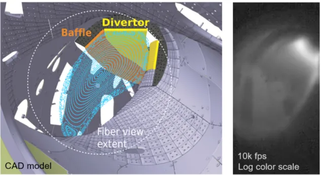
Figure 2-3: (Left) View of the MIT fast-camera with divertor panels labeled and a

cross-section of plasma flux surfaces superimposed. (Right) A single-frame snapshot

of plasma emission, showing the typical enhanced emission along the divertor

strike-line.

From this view, visible light from the cooler regions of the plasma—the boundary

and the divertor regions—is emitted and imaged by the camera, allowing plasma

fluctuations in those regions to be observed.

I was present on-site at W7-X during the installation of this diagnostic; as such, I

aided in the process as well. My role in the installation of the Phantom was primarily

to align the image-guide when we coupled it to the optical system that directed the

output of the image-guide to the two cameras. The image-guide was aligned on the

end pointing into the plasma vessel but needed alignment on the end connecting to

the diagnostic. Because the fibers in the image-guide were grouped together in a

rectangular format, alignment of the image-guide entailed illuminating that face of

the image-guide and rotating the bundle to match the desired angle for the rectangle,

and then pointing the guide in order to achieve the view as shown in Fig. 2-3 (Right).

2.3

Gas-Puff Imaging Diagnostic Standard

Gas-puff imaging diagnostics have been implemented on tokamak experiments such

as the National Spherical Torus Experiment (NSTX) and MIT’s Alcator C-Mod [7].

Both diagnostics on these experiments were similarly structured, with a controlled

neutral gas-puff, typically helium or deuterium, being injected at the edge of the

plasma [2]. The visible light emission from the gas cloud was then imaged with a

fast-camera in short exposures, “shorter than the autocorrelation time of the turbulence”,

where the images obtained in the radial vs. poloidal plane corresponded directly to the

instantaneous structure of the turbulence and followed the motion of the turbulence

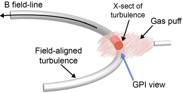
[7]. A schematic overview of this concept is shown in Fig. 2-4.

Figure 2-4: Overview of the mechanics for gas-puff imaging. The neutral gas is puffed

perpendicular to the local magnetic field, and the line emissions are then observed by

the fast-camera pointing parallel to the magnetic field at the point of interaction to

observe boundary turbulence [2].

Our GPI diagnostic implementation follows the standards set by previous

imple-mentations of the diagnostic, also containing a fast-camera component with framing

rates faster than the lifetime of turbulence in the plasma. This fast-camera component

will be coupled with a gas-puffing component in the sight-lines of the collecting optics.

The localized gas puff, either helium or deuterium, will interact with the boundary

plasma, exciting line emissions from the puffed-gas cloud. We use the 652 nm H𝛼 line

for H

gas and the 587 nm line from neutral helium when He gas is puffed, both of

which are the strongest lines in the visible spectrum for those elements. The emitted

light is collected in an appropriate geometry using high-throughput optics, which then

present a two-dimensional image of the emission to the camera system. Because the

light emission responds to fluctuations in the local electron density and temperature,

imaging the light fluctuations acts as a proxy for imaging the local plasma

fluctu-ations [7]. As such, turbulent behavior at the plasma boundary is captured by the

camera for further analysis.

Chapter 3

Design Methodology and Results

Because the GPI diagnostic contains multiple components and systems, each

individ-ual portion was selected by screening through different criteria and comparing with

various available options. The major design portions were selection of the port to

house the GPI, choosing which camera to use for the fast-camera subsystem, the

design of the gas injection subsystem, the design of the valve control and data

collec-tion subsystem, and various simulacollec-tions and tests leading to the Conceptual Design

Review (CDR) held at W7-X in April 2019. Information regarding the specifications

needed for W7-X and regarding aspects of W7-X itself was provided to us by Olaf

Grulke, Adrian von Stechow, and Christoph von Sehren.

3.1

Port Selection

The first priority of this diagnostic was to choose an appropriate port as its host,

which ideally would have the correct distance for our optical focus as well as provide

us with a good view near the last closed flux surface that would interact with the

puffed gas. Work to determine the ideal port began two years ago in the summer

of 2017, where we conducted sightline analyses for all available ports on W7-X, and

then narrowed down further through these following constraints:

(1) The sightline should be approximately aligned with the local magnetic field at

the location where the viewing chord intersects the gas puff;

(2) The view should be near the plasma boundary, i.e. within 0.05 m of the LCFS;

(3) The gas puff must not be too far from the viewing port since we must maximize

the signal to noise for the detected line emission from the puffed gas;

(4) It is optimal if the sightline is perpendicular to the local normal to the

flux-surface at the location where the sightline intersects the gas puff;

(5) Ideally the region viewed should be a region of interest with expected turbulence.

Following from initial work done by Seung-Gyou Baek, where all possible ports

with all possible views were considered, I subsequently narrowed down the selection

of possible ports by collapsing the views to an average sightline and investigating the

actual availability of ports. After further looking at CAD renderings of the plasma

vessel and realizing that many ports were occupied for heating purposes or for other

diagnostics, we eventually were able to consolidate the selections to five ports that

would still satisfy the above conditions, albeit through use of a turning mirror to

ensure the correct view from the first two conditions.

The five possible ports were AEE50, AEE11, AEK41, AEK10, and AEK50. Upon

closer inspection and consultation with Olaf Grulke, we determined that port AEE50

would be appropriate for our purposes, with the view directed towards AEK50. The

expected plasma cross-sectional view is shown in Appendix Fig. A-1. Port AEE50

will house the light-collecting optics for the fast-camera subsystem, while port AEK50

will host the gas-supplying capillary and the nozzle to puff the gas into the vessel near

the plasma boundary.

3.2

Fast-Camera Subsystem

For the fast-camera subsystem, we had the option of keeping our current camera, the

Phantom v710, or buying a much more sensitive camera that uses arrays of Avalanche

Photo-Diodes (APDs). Such an optimally-sensitive camera, called the

APDCAM-10G, is available commercially from a Hungarian company, Fusion Instruments, Inc.

We ultimately chose to purchase the APDCAM-10G because of its much higher

sensi-tivity. Even though we are striving to maximize the light-collection of the optics, we

are ultimately limited by the detected photon flux and thus need to maximize that.

The APDCAM-10G and its corresponding microlens array are shown in Fig. 3-1.

Figure 3-1: Fusion Instruments APDCAM-10G (left) and the microlens array (right).

This will be the camera we will be using for the GPI diagnostic, with a 4x8 microlens

array coupled to the camera for near 100% photon detection efficiency.

The two cameras and their respective optical setups, including various lenses, a

vacuum window to separate the more delicate aforementioned lenses from the inside of

the plasma vessel, and the turning mirror, were compared by conducting simulations

using Zemax OpticStudio. This software provided insight into aspects such as light

loss during transmission through the mirror and lenses before reaching the cameras,

the parameters of the optical elements, the relative placement of those elements,

and geometric image analyses. Because the detector areas of the two systems were

different, the two systems had different requirements for the magnification between

the image and the object planes. The detector size for the Phantom v710 was ∼4x4

mm, while the footprint for the APDCAM-10G detector was 23.4x39 mm. Therefore,

to image a roughly 50x70 mm area in object space corresponding to the gas puff

region, the required magnifications were ∼12 and ∼2 respectively.

In both cases, the optical distance between the object plane at the gas puff to

the vacuum window was held constant at about 1.4 meters, accurately reflecting the

physical constraints by the chosen ports and their distances to the plasma. Also, the

distance between the vacuum window and the camera was approximately constant

since the camera had to be located outside of the port flange. However, the other

optical elements were kept variable, with their separations optimized to provide the

most ideal focus at the camera detection planes with appropriate magnifications.

Partly as a result of these simulations, we decided on purchasing the APDCAM-10G.

3.2.1

Simulations for the Phantom v710 Optical Setup

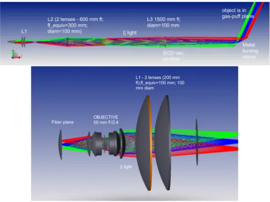
From the plasma to the Phantom v710, the intermediate optical system included

a large turning mirror, a vacuum window, a series of five focusing lenses, and an

objective lens to concentrate light onto the fiber which connects to the camera. This

portion of the optical setup is shown in Fig. 3-2, specifically for the 587 nm He line.

Figure 3-2: (Top) Optical system for the case where the Phantom v710 is chosen for

the GPI. Photons from the plasma in the top right are reflected by the angled turning

mirror, then channeled through the vacuum window, and finally through the series

of lenses to the focus of the camera on the far left. (Bottom) Zoomed in view of the

system of lenses and objective lens pictured in the far left of the overview.

Detailed specifications of the precise distances and other optical parameters

nec-essary to simulate the above system are shown in Appendix Table B.1. In this case,

the overall distance between the gas puff and the detection plane was approximately

2800 mm. Further details on the general characteristics of the system are available

in Appendix Fig. A-2, with one of the more important characteristics being that

this system had a paraxial magnification of 9.8. Although this was slightly under the

desired magnification of approximately 12, the difference was slight enough that it

was not significantly detrimental to the system.

Simulation results including a spot diagram to determine the effects of off-axis

objects on the image focus and a geometric encircled energy plot to determine the

fraction of enclosed photon energy based on radius on the image plane are shown in

Appendix Figs. A-3 and A-4. As seen from the image spot diagrams for single points

in the object plane, off-axis objects caused aberrations to the image, and the image

ended up being on the scale of 0.4 to 1.4 mm in size. The geometric encircled energy

plot shows over 90% of the photon energies being within an image spot of 0.35 mm

radius.

However, while the system seemed to be acceptable, upon closer inspection, it

turned out that photons were lost in the system, particularly in the objective lens,

due to the limiting geometric factors not allowing all of the photons at the edge of the

inner lenses to pass through. Due to the loss of photons in transit from the plasma

boundary to the detection plane, we sought for a better option.

3.2.2

Simulations for the APDCAM-10G Optical Setup

From the plasma to the APDCAM-10G, the intermediate optical system consisted of

a large turning mirror, a vacuum window, and only three focusing lenses to direct

light onto the detector of the camera. The small magnification, being approximately

2, caused this system to be much less complicated than that for the Phantom v710.

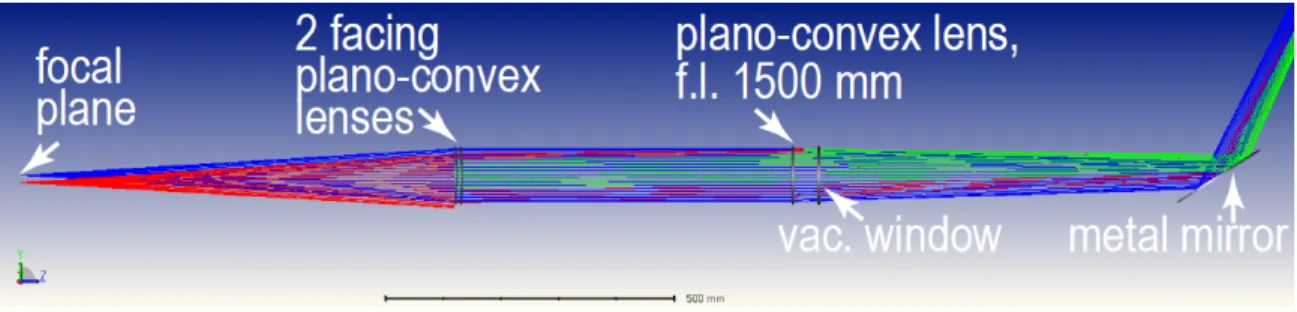
The overview of this optical setup is shown in Fig. 3-3, specifically for the 587 nm

He line.

neces-Figure 3-3: Optical system for the case where the APDCAM-10G is chosen for the

GPI. Photons from the plasma in the top right are reflected by the angled turning

mirror, then channeled through the vacuum window, and through three lenses to

focus onto the camera.

sary to simulate the above system are shown in Appendix Table B.2. In this case, the

overall distance between the gas puff and the detection plane was also approximately

2800 mm as required. Further details on the general characteristics of the system are

available in Appendix Fig. A-5, with one of the more important characteristics being

that this system had a paraxial magnification of approximately 2, as desired.

Similar to the simulations run for the Phantom v710, an image spot diagram and

a geometric encircled energy plot for points in object space were generated, and they

are shown in Appendix Figs. A-6 and A-7. From the spot diagram, off-axis objects

caused slight aberrations to the image as well, but the image still ended up being

about 0.1 to 0.2 mm in size, well within the size constraints of the detector. The

geometric encircled energy plot further supported this, with over 90% of the photon

energies being within 0.06 mm of the radius of the image spot.

Similar to the Phantom v710 system, this configuration also faced some loss of

photons during transmission. However, because of the simpler design with a fewer

number of lenses, the magnitude of photons lost was not as significant. Moreover,

because of the excellent focus onto the detector and the near-perfect efficiency of the

detector, the APDCAM-10G system outperformed the Phantom v710 configuration

to become our camera of choice.

3.3

Gas-Puff Valve Subsystem

For the gas-puffing subsystem, we needed a system that would contain and store the

gas until a puff is to be released into the plasma vessel in a fast manner, while also

having the capability of keeping track of absolute and differential pressures within

the system to determine how much gas is released into the vessel per puff. A CAD

rendering of all of the components for this subsystem is shown in Fig. 3-4.

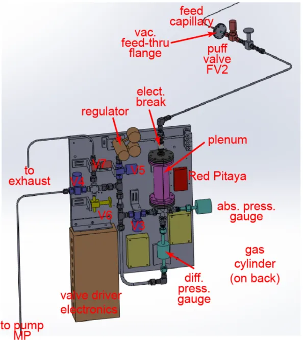
Figure 3-4: CAD rendering of the gas-puff valve subsystem with all of the components

in place on the mounting plate.

As seen in the rendering, there are multiple components that make up the

sub-system as a whole.

(1) To store the gas, there is a replaceable gas cylinder on the back of the mounting

plate (not visible in Fig. 3-4) that provides gas for the system.

(2) To control the flow of the gas, a series of bellows-sealed pneumatically actuated

valves are utilized. These valves were purchased from Swagelok—FV2 is the

“in-jection” valve that opens and closes quickly to release gas into the feed capillary,

which goes to the nozzle and into the plasma vessel, while V3, V4, and V5 are

“slow” valves which facilitate the transfer of gas within the main valve system

to the plenum or to the vacuum pump. The plenum serves as the reservoir for

the gas being injected and provides backing pressure for the injection.

(3) To keep track of how much gas is in the valve system and how much is released

into the plasma vessel, an absolute pressure gauge and a differential pressure

gauge from MKS were purchased, since the amount of gas held in the system

correlates directly to the pressure within.

(4) To be able to control the Swagelok valves electronically, we purchased

pneu-matic solenoid valves from Nupneu-matics, which serve as links between electrical

commands and physically actuating the Swagelok valves to open and close.

These valves are mounted on the top right of the plate and connect to the

Swagelok valves through tubes that allow air to be forced from the solenoid

valves to actuate the Swagelok valves.

(5) To be able to control the Numatics valves remotely, we utilize a Red Pitaya

field-programmable gate array (FPGA). The Red Pitaya is also a computer and

is therefore on the network and in principle can be accessed from any other

computer on the network. The Red Pitaya also digitizes the data from the

pressure gauges, therefore allowing measurement and archival of how much gas

is released to the vessel.

(6) Because the input/output pins on the Red Pitaya have set voltage limitations

that are insufficient for the solenoid valves, an intermediate system through the

valve driver electronics is needed. In those control circuits, the 3.3 V signals

from the Red Pitaya are taken and amplified to the 24 V needed for solenoid

valve control. The control circuit for the fast valve also includes inputs for

timing triggers and permission from W7-X to release gas into the vessel.

(7) For safety purposes, there is a regulator and an electrical break.

Much of the initial design and refinement of the system was done by James L.

Terry, though I was able to help in choosing to purchase the Numatics solenoid

valves and the parts needed to connect them to the Swagelok valves. I also aided

in physically assembling the main part of the subsystem on the bench, including

designing the mounting brackets and holding structures.

3.4

Valve Control and Data Collection Subsystem

For the valve control and data collection subsystem, we opted to create a Python

graphical user interface (GUI) coupled with programming a Red Pitaya STEMlab

125-14 FPGA board. As seen in the previous section, the Red Pitaya is to be mounted

alongside the gas-puff valve subsystem and connected to the valve driver electronics

to be able to drive the solenoid valves. As noted above, the Red Pitaya also takes

in readings from the absolute and differential pressure gauges as well as inputs from

W7-X about timing triggers and firing permissions.

3.4.1

Red Pitaya Field-Programmable Gate Array

Programming the Red Pitaya FPGA entailed sending the Red Pitaya a blueprint of

how to rearrange its structure and what signals to respond to, as it is an integrated

circuit designed to be configured by the consumer on the field. With the guidance of

PhD Student William McCarthy, I was able to take charge in the design of the Red

Pitaya. A schematic overview of the Red Pitaya is shown in Fig. 3-5.

Figure 3-5: General schematic of the Red Pitaya STEMlab 125-14 components. The

Red Pitaya has on-board processor and FPGA, along with RAM and network

con-nectivity on top of customizable pins in the extension connectors [3].

The Red Pitaya features two fast-digitizing analog inputs and two analog outputs.

Furthermore, the Red Pitaya also contains four slow analog inputs and four outputs,

but those pins were not available during FPGA programming. As such, we utilized

the remaining 16 single ended digital input/output pins. The schematic of the Red

Pitaya extension connector pinout is shown in Fig.3-6.

Figure 3-6: Detailed pin descriptions of the extension connectors [4].

to set up the pins, components, and variables needed, and then connected appropriate

pins to locations within blocks and vice versa, with the general connections as shown

in Fig. 3-7. The Vivado detailed result is shown in Appendix Fig. A-8.

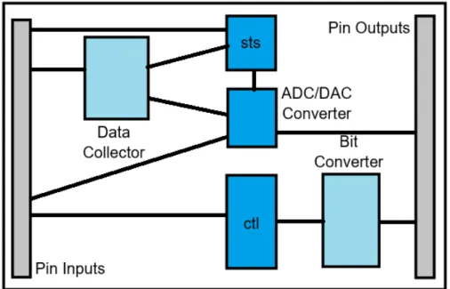
Figure 3-7: General overview of the FPGA design layout.

The pins are represented by the gray areas on the far left and far right, while the

inner blocks represent specific functions taken between pins. Notably, the sts block

represents the status register, which accepts signals to set internal states within the

FPGA. The ctl block represents the control register, which passes signals outward

to the pins, thereby controlling them. However, because the signals sent by the

control register are 32 bits, while only 1 bit is needed to control the output pins, an

intermediate bit converter block is needed to truncate the signal for the pins.

Various pieces of code were needed to generate the design in Vivado Design Suite

and served different purposes in programming the FPGA pins to the appropriate

variables and to set functions available to us from the software end. The code is

shown in Appendix C, with the functions as follows:

• block_design.tcl (Appendix C-1): This is the overall block design file that allows

Vivado Design Suite to generate the graphical version shown in Appendix Fig.

A-8. All additions of blocks, pins, and connections are done in this file.

• config.yml (Appendix C-2): This is the configuration file for Vivado Design

Suite, which provides settings such as the cores/blocks to be used, the control

and status registers, and other parameters.

• extension_connector.xdc (Appendix C-3): This defines the digital I/O pins

from the Red Pitaya and maps them to corresponding internal variables.

• GPI_2.hpp (Appendix C-4): This is a C++ header file that creates all of the

functions to read and write to the status and control registers through the

variable names set in the block design and the extension connector files. This

file also defines the functions needed for data collection.

• GPI_2.py (Appendix C-5): This is a Python file that links to the previous

header file, mapping Python functions to the functions within the header file.

With this, we can control the FPGA using Python scripts. The data collection

functions were not implemented in this file at the time.

• DataCollect.vhd (Appendix C-6): This sets up the data collection block. The

original file was provided by William McCarthy for his “Mirror Langmuir Probe”

project and the file has been simplified since.

• outputs.vhd (Appendix C-7): This sets up the intermediate block to process

the signal from the control register to the outbound pins.

With all of these files in place, the FPGA design was uploaded to the Red Pitaya

successfully. Subsequent work with the design was picked up by Sean Ballinger to

complete the implementation of the data collection functions.

3.4.2

Python Graphical User Interface

To control the Red Pitaya’s functions from a computer, I created a GUI in Python

using the ‘Tkinter’ library. The GUI is shown in Fig. 3-8.

The Python GUI shows a stripped down overview of the valve system as well as

specific statuses of the valves and W7-X. With this GUI, it is possible to control each

Figure 3-8: Overview of the Python GUI.

of the four valves manually, opening and closing them individually. However, it is also

possible to set automatic timings for the valves to open and close, releasing gas into

the plasma vessel at set instances and for set durations after receiving permission

and timing triggers from W7-X. The boxes on the right are for readings from the

differential and absolute pressure gauges, which measure how much gas is stored in

the system and how much gas is injected through the “injection” valve, FV2. The

GUI coupled with the FPGA allows the system to automatically fill or refill to a user

inputted desired pressure, and stores relevant data to the server.

The GUI is able to communicate with the Red Pitaya through a network

con-nection and then calls upon the Python functions written for the FPGA control as

mentioned in the previous section. Thus, the various abilities seen on the front-end

of the GUI are mapped to functions in the Red Pitaya through the back-end. The

code to generate the GUI is shown in Appendix C-8.

Subsequent work was taken up by Sean Ballinger, completing the graphing

mech-anisms for readings from the pressure gauges and the automatic filling functionality.

3.5

Heat Loading Simulations

In order to determine the heat loads experienced by the plasma-facing components of

the diagnostic, which would, in turn, determine the design for cooling mechanisms,

heat loading simulations were conducted using the COMSOL Multiphysics code. This

is a finite element code. Because of W7-X’s long-term goal of attaining steady-state

operation for 30 minutes, it is imperative that the diagnostic’s components will be

kept within safe operating limits. The simulations included steady-state runs for

the gas puffing nozzle at AEK50 and for the overall optical system within AEE50.

All of the modeling assumed a 100 kW/m

radiative heat load emanating from the

plasma. The heat load is the maximum expected during the steady-state operation

phase of W7-X. In the COMSOL thermal modeling, the heat load was simulated as

a blackbody sheet radiating at 880°C roughly 200 mm beyond the port entrances.

3.5.1

Heat Load Analysis of the Gas Puff Nozzle

With the gas puffing nozzle as designed by James L. Terry, running the steady-state

heat load simulation results in the temperature distribution shown in Fig. 3-9.

This steady-state simulation was run with the boundary condition that the bracket

on which the nozzle structure is fastened is in contact with a surface being held at

30°C, as indicated by the dark blue region on the left in Fig. 3-9. The nozzle’s

material was graphite, while everything else was modeled as stainless steel. With

those thermal properties, the gas puff nozzle reaches a maximum of 590°C at its

plasma-facing surface.

In an effort to reduce the peak temperature of the gas puffing nozzle, another

COMSOL simulation was run with the nozzle design as shown in Fig. 3-10.

Figure 3-10: COMSOL analysis of an idealized situation for the gas puff nozzle with

a larger fraction of the mounting bracket cooled to 30°C.

Material conditions were the same as the previous simulation, with the nozzle

component made from graphite and everything else being stainless steel. With

ad-ditional cooling at 30°C provided to the nozzle (to the right of the nozzle as seen in

Fig. 3-10) through the mounting bracket, the maximum temperature reached on the

face of the nozzle is 400°C. Because this situation is not realistic, as it would be very

difficult to provide appropriate cooling to the nozzle on that side which is not directly

attached to the port wall, this constitutes the best-case scenario.

With the peak temperature of the nozzle being about 600°C, even though that

is not the best case scenario, the W7-X engineers believe that this should not be a

danger to machine operation, nor should it damage the nozzle structure.

3.5.2

Heat Load Analysis of the Immersion Tube

Port AEE50 hosts the immersion tube which constitutes the vacuum interface and

houses the optical system. Due to the sensitive elements within the component, it is

imperative that temperatures do not reach high enough to compromise the vacuum

window (whose maximum tolerance for temperature is 200°C), or affect the

perfor-mance of the lenses or turning mirror. A steady-state simulation including

water-cooling pipes to the tube portion beyond the vacuum window (but not extending to

the shutter/turning mirror box at the plasma end of the immersion tube) resulted in

Fig. 3-11.

Figure 3-11: COMSOL analysis of the optical system with one set of cooling pipes.

Port AEE50 can be seen on the left, while the 880°C plasma sheet can be seen on the

right.

cooling for the gas puff nozzle. All components in this simulation were modeled after

stainless steel. In this configuration, the front face of the shutter box, which also hosts

the turning mirror, reaches about 570°C. The vacuum window connecting the bigger

tube to the smaller tube reaches about 230°C. While the shutter box can withstand

temperatures of that scale, the vacuum window should be below 200°C to be within

safety margins.

As such, a subsequent steady-state simulation with a second set of cooling pipes

added resulted in Fig. 3-12.

Figure 3-12: COMSOL analysis of the optical system with two sets of cooling pipes

flanking the vacuum window to cool the length of the tube as much as possible and

therefore the window as well.

With the two sets of cooling pipes, the shutter box still reaches about 570°C but

the vacuum window is about 175°C, now within the safety margins. Thus, we found

that two sets of cooling pipes are necessary to keep the window, the tubes, and optical

elements sufficiently cooled.

Chapter 4

Summary

At present most of the individual components of the GPI diagnostic have been

de-signed. CAD renderings of the system as presently designed and mounted onto W7-X

are shown in Figs. 4-1 and 4-2. In Fig. 4-1 the roles of each of the subsystems are

labeled.

Figure 4-1: Overview of all of the components of the GPI diagnostic in place at their

respective port locations.

Figure 4-2: Overview of the entire GPI diagnostic from a different angle than in Fig.

4-1. The sightline intersecting with the injected gas can be clearly seen.

Within the overall design of the entire diagnostic and the past two years of working

with the group, I now summarize my main roles in the project:

1. On-site at W7-X in Germany, I helped install the fast-framing camera

diagnos-tic. I performed the alignment of the camera system with the image-guide.

2. I helped narrow down the selection of ports in the initial search for suitable

ports on which to mount the GPI diagnostic.

3. I performed simulations of the optical system using Zemax OpticStudio for both

the Phantom v710 and APDCAM-10G cases.

4. I helped assemble the gas-puff valve subsystem.

5. I was responsible for programming the Red Pitaya FPGA and its corresponding

Python GUI.

6. I performed finite element code simulations of the expected heat loads on the

gas puffing nozzle and the immersion tube that houses the optical system and

the vacuum window. The code used was COMSOL Multiphysics.

The fast-framing camera has run routinely and successfully on W7-X since its

installation. The GPI diagnostic has passed W7-X’s Conceptual Design Review.

Although it must still pass a Final Design Review and have the remaining components

fabricated or procured, it is on track to be installed onto W7-X by the beginning of

its second operation phase in 2021.

Appendix A

Figures

Figure A-1: Plasma cross section at the toroidal angle of the gas puff nozzle at port

AEK50. Prominent plasma features such as the LCFS in blue and plasma islands in

red are also shown.

Figure A-2: Various details for general characteristics of the Zemax simulated

Phan-tom v710 optical system.

Figure A-3: Spot diagram for the Phantom v710 simulation. The image on the top

left is that of the on-axis object, whereas the other two correspond to off-axis objects.

We can thus see that the focused image spot is at best 0.4 mm in size and at worst

1.4 mm, which is acceptable for the 4x4 mm detector.

Figure A-4: Geometric encircled energy plot for the Phantom v710 simulation. The

on-axis case reaches 100% enclosed photon energy at around 0.34 mm, while the

off-axis cases reach about 90% at that point.

Figure A-5: Various details for general characteristics of the Zemax simulated

APDCAM-10G optical system.

Figure A-6: Spot diagram for the APDCAM-10G simulation. The image on the top

left is that of the on-axis object, whereas the other two correspond to off-axis objects.

We can thus see that the focused image spot is at best 0.1 mm in size and at worst

0.2 mm, which is well acceptable for the 23.4x39 mm detector.

Figure A-7: Geometric encircled energy plot for the APDCAM-10G simulation. The

on-axis case reaches 100% enclosed photon energy at around 0.055 mm, while the

off-axis cases reach about 90% at that point.

Figure

A-8:

Ov

erview

of

the

FPGA

design

in

Viv

ado

Design

Suite.

Appendix B

Tables

Table B.1: Detailed specification of the various distances and parameters necessary to

generate the optical system for the Phantom v710 case. The radius column refers to

the radius of curvature of the optical elements, the thickness the distance separation

between two faces of those elements, and the semi-diameter their radial size, all of

which are in mm. The materials were selected to have the same optical qualities as

those that would be actually used and blank materials indicate air. These values have

been optimized within Zemax to provide the best focus at the detection plane. The

overall distance between the gas puff and the detection plane is approximately 2800

mm.

Table B.2: Detailed specification of the various distances and parameters necessary

to generate the optical system for the APDCAM-10G case. The columns are defined

the same way as those in Table B.1. These values have been optimized within Zemax

to provide the best focus at the detection plane. The overall distance between the

gas puff and the detection plane is also approximately 2800 mm.

Appendix C

Code and Scripts

C.1

block_design.tcl

s o u r c e $board_path/ c o n f i g / p o r t s . t c l # Add PS and AXI I n t e r c o n n e c t

s e t board_preset $board_path/ c o n f i g / board_preset . t c l s o u r c e $sdk_path/ fpga / l i b / s t a r t i n g _ p o i n t . t c l

# Add ADCs and DACs

s o u r c e $sdk_path/ fpga / l i b /redp_adc_dac . t c l s e t adc_dac_name adc_dac

add_redp_adc_dac $adc_dac_name # Rename c l o c k s

s e t adc_clk $adc_dac_name/ adc_clk

# Add p r o c e s s o r system r e s e t synchronous to adc c l o c k s e t rst_adc_clk_name proc_sys_reset_adc_clk

c e l l x i l i n x . com : i p : proc_sys_reset : 5 . 0 $rst_adc_clk_name {} { ext_reset_in $ps_name/FCLK_RESET0_N

slowest_sync_clk $adc_clk }

# Add c o n f i g and s t a t u s r e g i s t e r s s o u r c e $sdk_path/ fpga / l i b / c t l _ s t s . t c l

add_ctl_sts $adc_clk $rst_adc_clk_name/ p e r i p h e r a l _ a r e s e t n # Connect LEDs

# Connect ADC to s t a t u s r e g i s t e r

f o r { s e t i 0} { $ i < [ get_parameter n_adc ] } { i n c r i } { connect_pins [ sts_pin adc$i ] adc_dac/ adc [ expr $ i + 1 ] }

## Add DAC c o n t r o l l e r

#s o u r c e $sdk_path/ fpga / l i b /bram . t c l #s e t dac_bram_name [ add_bram dac ]

#connect_pins adc_dac/ dac1 [ get_slice_pin $dac_bram_name/ doutb 13 0 ] #connect_pins adc_dac/ dac2 [ get_slice_pin $dac_bram_name/ doutb 29 1 6 ] #c o n n e c t _ c e l l $dac_bram_name { # web [ get_constant_pin 0 4 ] # dinb [ get_constant_pin 0 3 2 ] # clkb $adc_clk # r s t b $rst_adc_clk_name/ p e r i p h e r a l _ r e s e t #}

# Use AXI Stream c l o c k c o n v e r t e r (ADC c l o c k −> FPGA c l o c k ) s e t intercon_idx 0

s e t idx [ add_master_interface $intercon_idx ]

c e l l x i l i n x . com : i p : axis_clock_converter : 1 . 1 adc_clock_converter { TDATA_NUM_BYTES 4

} {

s_axis_aresetn $rst_adc_clk_name/ p e r i p h e r a l _ a r e s e t n

m_axis_aresetn [ s e t r s t $ { intercon_idx }_name] / p e r i p h e r a l _ a r e s e t n s_axis_aclk $adc_clk

m_axis_aclk [ s e t ps_clk$intercon_idx ] }

# Add AXI stream FIFO to read p u l s e data from the PS c e l l x i l i n x . com : i p : axi_fifo_mm_s : 4 . 1 adc_axis_fifo {

C_USE_TX_DATA 0 C_USE_TX_CTRL 0 C_USE_RX_CUT_THROUGH t r u e C_RX_FIFO_DEPTH 32768 C_RX_FIFO_PF_THRESHOLD 32760 } { s_axi_aclk [ s e t ps_clk$intercon_idx ]

s_axi_aresetn [ s e t r s t $ { intercon_idx }_name] / p e r i p h e r a l _ a r e s e t n S_AXI [ s e t interconnect_$ { intercon_idx }_name] /M${ idx }_AXI AXI_STR_RXD adc_clock_converter /M_AXIS

}

assign_bd_address [ get_bd_addr_segs adc_axis_fifo /S_AXI/Mem0]

s e t memory_segment [ get_bd_addr_segs /$ { : : ps_name}/Data/SEG_adc_axis_fifo_Mem0 ] set_property o f f s e t [ get_memory_offset a d c _ f i f o ] $memory_segment

set_property range [ get_memory_range a d c _ f i f o ] $memory_segment

############################# Make a l l the Blocks ################################## create_bd_cell −type ip −vlnv PSFC: u se r : d a t a _ c o l l e c t o r : 1 . 0 data_collector_0

create_bd_cell −type ip −vlnv x i l i n x . com : ip : x l c o n s t a n t : 1 . 1 xlconstant_0

############################# Connected a l l the Blocks ############################# connect_bd_net [ get_bd_pins data_collector_0 / tdata ]

[ get_bd_pins adc_clock_converter / s_axis_tdata ] connect_bd_net [ get_bd_pins data_collector_0 / t v a l i d ]

[ get_bd_pins adc_clock_converter / s_axis_tvalid ]

connect_bd_net [ get_bd_pins data_collector_0 / adc_clk ] [ get_bd_pins adc_dac/ adc_clk ] connect_bd_net [ get_bd_pins xlconstant_0 / dout ] [ get_bd_pins data_collector_0 / clk_en ] # Connect ADC p i n s to p r e s s u r e gauge s t a t u s r e g i s t e r s

connect_bd_net [ get_bd_pins adc_dac/ adc1 ] [ get_bd_pins s t s /abs_gauge ] −boundary_type upper

connect_bd_net [ get_bd_pins adc_dac/ adc2 ] [ get_bd_pins s t s / diff_gauge ] −_{boundary_type upper}

# Add p i n s from e x t e n s i o n c o n n e c t o r s create_bd_port −d i r I W7X_permission_in create_bd_port −d i r I W7X_timings

create_bd_port −d i r O −from 0 −to 0 slow_1_trigger create_bd_port −d i r O −from 0 −to 0 slow_2_trigger create_bd_port −d i r O −from 0 −to 0 slow_3_trigger create_bd_port −d i r O −from 0 −to 0 slow_4_trigger create_bd_port −d i r O −from 0 −to 0 f a s t _ 1 _ t r i g g e r create_bd_port −d i r O −from 0 −to 0 fast_1_permission_1 create_bd_port −d i r O −from 0 −to 0 fast_1_duration_1 create_bd_port −d i r O −from 0 −to 0 fast_1_permission_2 create_bd_port −d i r O −from 0 −to 0 fast_1_duration_2 create_bd_port −d i r O −from 0 −to 0 f a s t _ 2 _ t r i g g e r create_bd_port −d i r O −from 0 −to 0 fast_2_permission_1 create_bd_port −d i r O −from 0 −to 0 fast_2_duration_1 create_bd_port −d i r O −from 0 −to 0 fast_2_permission_2 create_bd_port −d i r O −from 0 −to 0 fast_2_duration_2

# Add block which p r o c e s s e s the outputs

create_bd_cell −type ip −vlnv PSFC: u se r : outputs : 1 . 0 outputs_0 # Connect output p i n s

connect_bd_net [ get_bd_pins adc_dac/ adc_clk ] [ get_bd_pins outputs_0 / adc_clk ]

connect_bd_net [ get_bd_pins c t l / GPI_safe_state ] [ get_bd_pins outputs_0 / GPI_safe_state_ctl ] connect_bd_net [ get_bd_pins c t l / slow_1_trigger ]

[ get_bd_pins outputs_0 / slow_1_trigger_ctl ] connect_bd_net [ get_bd_pins c t l / slow_2_trigger ]

[ get_bd_pins outputs_0 / slow_2_trigger_ctl ] connect_bd_net [ get_bd_pins c t l / slow_3_trigger ]

[ get_bd_pins outputs_0 / slow_3_trigger_ctl ] connect_bd_net [ get_bd_pins c t l / slow_4_trigger ]

[ get_bd_pins outputs_0 / slow_4_trigger_ctl ] connect_bd_net [ get_bd_ports W7X_permission_in ]

[ get_bd_pins outputs_0 /W7X_permission_out_ctl ] connect_bd_net [ get_bd_pins c t l / f a s t _ 1 _ t r i g g e r ]

[ get_bd_pins outputs_0 / f a s t _ 1 _ t r i g g e r _ c t l ] connect_bd_net [ get_bd_pins c t l / fast_1_permission_1 ]

[ get_bd_pins outputs_0 / fast_1_permission_1_ctl ] connect_bd_net [ get_bd_pins c t l / fast_1_duration_1 ]

[ get_bd_pins outputs_0 / fast_1_duration_1_ctl ] connect_bd_net [ get_bd_pins c t l / fast_1_permission_2 ]

[ get_bd_pins outputs_0 / fast_1_permission_2_ctl ] connect_bd_net [ get_bd_pins c t l / fast_1_duration_2 ]

[ get_bd_pins outputs_0 / fast_1_duration_2_ctl ] connect_bd_net [ get_bd_pins c t l / f a s t _ 2 _ t r i g g e r ]

[ get_bd_pins outputs_0 / f a s t _ 2 _ t r i g g e r _ c t l ] connect_bd_net [ get_bd_pins c t l / fast_2_permission_1 ]

[ get_bd_pins outputs_0 / fast_2_permission_1_ctl ] connect_bd_net [ get_bd_pins c t l / fast_2_duration_1 ]

[ get_bd_pins outputs_0 / fast_2_duration_1_ctl ] connect_bd_net [ get_bd_pins c t l / fast_2_permission_2 ]

[ get_bd_pins outputs_0 / fast_2_permission_2_ctl ] connect_bd_net [ get_bd_pins c t l / fast_2_duration_2 ]

[ get_bd_pins outputs_0 / fast_2_duration_2_ctl ] connect_bd_net [ get_bd_ports slow_1_trigger ]

[ get_bd_pins outputs_0 / slow_1_trigger_pin ] connect_bd_net [ get_bd_ports slow_2_trigger ]

[ get_bd_pins outputs_0 / slow_2_trigger_pin ] connect_bd_net [ get_bd_ports slow_3_trigger ]

connect_bd_net [ get_bd_ports slow_4_trigger ] [ get_bd_pins outputs_0 / slow_4_trigger_pin ] connect_bd_net [ get_bd_ports f a s t _ 1 _ t r i g g e r ]

[ get_bd_pins outputs_0 / fast_1_trigger_pin ] connect_bd_net [ get_bd_ports fast_1_permission_1 ]

[ get_bd_pins outputs_0 / fast_1_permission_1_pin ] connect_bd_net [ get_bd_ports fast_1_duration_1 ]

[ get_bd_pins outputs_0 / fast_1_duration_1_pin ] connect_bd_net [ get_bd_ports fast_1_permission_2 ]

[ get_bd_pins outputs_0 / fast_1_permission_2_pin ] connect_bd_net [ get_bd_ports fast_1_duration_2 ]

[ get_bd_pins outputs_0 / fast_1_duration_2_pin ] connect_bd_net [ get_bd_ports f a s t _ 2 _ t r i g g e r ]

[ get_bd_pins outputs_0 / fast_2_trigger_pin ] connect_bd_net [ get_bd_ports fast_2_permission_1 ]

[ get_bd_pins outputs_0 / fast_2_permission_1_pin ] connect_bd_net [ get_bd_ports fast_2_duration_1 ]

[ get_bd_pins outputs_0 / fast_2_duration_1_pin ] connect_bd_net [ get_bd_ports fast_2_permission_2 ]

[ get_bd_pins outputs_0 / fast_2_permission_2_pin ] connect_bd_net [ get_bd_ports fast_2_duration_2 ]

[ get_bd_pins outputs_0 / fast_2_duration_2_pin ]

connect_bd_net [ get_bd_pins outputs_0 / GPI_safe_state_pin ] [ get_bd_pins adc_dac/ dac1 ] connect_bd_net [ get_bd_pins outputs_0 /W7X_permission_out_pin ]

C.2

config.yml

−−−

name : GPI_2

board : boards / red−pitaya v e r s i o n : 0 . 1 . 1 c o r e s : − _{fpga / c o r e s /redp_adc_v1_0} − fpga / c o r e s /redp_dac_v1_0 − _{fpga / c o r e s / axi_ctl_register_v1_0} − _{fpga / c o r e s / axi_sts_register_v1_0} − fpga / c o r e s /dna_reader_v1_0

− instruments /GPI_2/ c o r e s / data_collector_v1_0 − _{instruments /GPI_2/ c o r e s /outputs_v1_0}

memory : − _{name : c o n t r o l} o f f s e t : ’0 x60000000 ’ range : 4K − _{name : s t a t u s} o f f s e t : ’0 x50000000 ’ range : 4K − name : dac o f f s e t : ’0 x40000000 ’ range : 32K − name : a d c _ f i f o o f f s e t : ’0 x43C10000 ’ range : 64K c o n t r o l _ r e g i s t e r s : − _{l e d} − _{GPI_safe_state} − slow_1_trigger − _{slow_2_trigger} − _{slow_3_trigger} − slow_4_trigger − _{f a s t _ 1 _ t r i g g e r} − _{fast_1_permission_1} − fast_1_duration_1 − fast_1_permission_2 − _{fast_1_duration_2} − _{f a s t _ 2 _ t r i g g e r} − fast_2_permission_1 − _{fast_2_duration_1}

− _{fast_2_permission_2} − _{fast_2_duration_2} s t a t u s _ r e g i s t e r s : − _{adc [ n_adc ]} − W7X_permission_in − _{W7X_timings} − _{abs_gauge} − diff_gauge parameters : f c l k 0 : 166666667 bram_addr_width : 13 dac_width : 14 adc_width : 14 n_adc : 2 xdc : − boards / red−pitaya / c o n f i g / p o r t s . xdc − boards / red−pitaya / c o n f i g / c l o c k s . xdc − _{instruments /GPI_2/ extension_connector . xdc} d r i v e r s : − _{. / GPI_2 . hpp} − s e r v e r / d r i v e r s /common . hpp # web : # − web/ koheron . t s # − web/ jquery . f l o t . d . t s # − _{. / web/ pulse_generator . t s} # − _{. / web/app . t s} # − . / web/ c o n t r o l . t s # − _{. / web/ p l o t . t s} # − _{. / web/ index . html} # − web/main . c s s # − web/ n a v i g a t i o n . t s

C.3

extension_connector.xdc

### Adding a l l o f the n e c e s s a r y p i n s from the e x t e n s i o n c o n n e c t o r s set_property IOSTANDARD LVCMOS33 [ get_ports W7X_permission_in ] set_property IOSTANDARD LVCMOS33 [ get_ports W7X_timings ] set_property PACKAGE_PIN G17 [ get_ports W7X_permission_in ] set_property PACKAGE_PIN H16 [ get_ports W7X_timings ]

set_property IOSTANDARD LVCMOS33 [ get_ports { slow_1_trigger [ 0 ] } ] set_property IOSTANDARD LVCMOS33 [ get_ports { slow_2_trigger [ 0 ] } ] set_property IOSTANDARD LVCMOS33 [ get_ports { slow_3_trigger [ 0 ] } ] set_property IOSTANDARD LVCMOS33 [ get_ports { slow_4_trigger [ 0 ] } ] set_property IOSTANDARD LVCMOS33 [ get_ports { f a s t _ 1 _ t r i g g e r [ 0 ] } ] set_property IOSTANDARD LVCMOS33 [ get_ports { fast_1_permission_1 [ 0 ] } ] set_property IOSTANDARD LVCMOS33 [ get_ports { fast_1_duration_1 [ 0 ] } ] set_property IOSTANDARD LVCMOS33 [ get_ports { fast_1_permission_2 [ 0 ] } ] set_property IOSTANDARD LVCMOS33 [ get_ports { fast_1_duration_2 [ 0 ] } ] set_property IOSTANDARD LVCMOS33 [ get_ports { f a s t _ 2 _ t r i g g e r [ 0 ] } ] set_property IOSTANDARD LVCMOS33 [ get_ports { fast_2_permission_1 [ 0 ] } ] set_property IOSTANDARD LVCMOS33 [ get_ports { fast_2_duration_1 [ 0 ] } ] set_property IOSTANDARD LVCMOS33 [ get_ports { fast_2_permission_2 [ 0 ] } ] set_property IOSTANDARD LVCMOS33 [ get_ports { fast_2_duration_2 [ 0 ] } ] set_property PACKAGE_PIN J18 [ get_ports { slow_1_trigger [ 0 ] } ]

set_property PACKAGE_PIN K17 [ get_ports { slow_2_trigger [ 0 ] } ] set_property PACKAGE_PIN L14 [ get_ports { slow_3_trigger [ 0 ] } ] set_property PACKAGE_PIN L16 [ get_ports { slow_4_trigger [ 0 ] } ] set_property PACKAGE_PIN G18 [ get_ports { f a s t _ 1 _ t r i g g e r [ 0 ] } ] set_property PACKAGE_PIN H17 [ get_ports { fast_1_permission_1 [ 0 ] } ] set_property PACKAGE_PIN H18 [ get_ports { fast_1_duration_1 [ 0 ] } ] set_property PACKAGE_PIN K18 [ get_ports { fast_1_permission_2 [ 0 ] } ] set_property PACKAGE_PIN L15 [ get_ports { fast_1_duration_2 [ 0 ] } ] set_property PACKAGE_PIN L17 [ get_ports { f a s t _ 2 _ t r i g g e r [ 0 ] } ] set_property PACKAGE_PIN J16 [ get_ports { fast_2_permission_1 [ 0 ] } ] set_property PACKAGE_PIN M15 [ get_ports { fast_2_duration_1 [ 0 ] } ] set_property PACKAGE_PIN K16 [ get_ports { fast_2_permission_2 [ 0 ] } ] set_property PACKAGE_PIN M14 [ get_ports { fast_2_duration_2 [ 0 ] } ]

C.4

GPI_2.hpp

// http : / /www. x i l i n x . com/ support / documentation / ip_documentation / axi_fifo_mm_s/v4_1/pg080−axi−f i f o −mm−s . pdf namespace Fifo_regs { constexpr uint32_t r d f r = 0x18 ; constexpr uint32_t r d f o = 0x1C ; constexpr uint32_t rdfd = 0x20 ; constexpr uint32_t r l r = 0x24 ; }

constexpr uint32_t dac_size = mem : : dac_range/ s i z e o f ( uint32_t ) ; constexpr uint32_t adc_buff_size = 16777216;

c l a s s GPI_2 { p u b l i c : GPI_2( Context& ctx_ ) : ctx ( ctx_ ) , c t l ( ctx .mm. get<mem : : c o n t r o l >()) , s t s ( ctx .mm. get<mem : : s t a t us >())

, adc_fifo_map ( ctx .mm. get<mem : : adc_fifo >()) , adc_data ( adc_buff_size )

// , dac_map( ctx .mm. get<mem : : dac >()) {

s t a r t _ f i f o _ a c q u i s i t i o n ( ) ; }

// GPI_2 g e n e r a t o r

void set_led ( uint32_t l e d ) { c t l . write <reg : : led >( l e d ) ; }