HAL Id: inserm-00130947
https://www.hal.inserm.fr/inserm-00130947
Submitted on 2 Mar 2007HAL is a multi-disciplinary open access archive for the deposit and dissemination of sci-entific research documents, whether they are pub-lished or not. The documents may come from teaching and research institutions in France or abroad, or from public or private research centers.
L’archive ouverte pluridisciplinaire HAL, est destinée au dépôt et à la diffusion de documents scientifiques de niveau recherche, publiés ou non, émanant des établissements d’enseignement et de recherche français ou étrangers, des laboratoires publics ou privés.
Ray casting with ”on-the-fly” region growing: 3-D
navigation into cardiac MSCT volume.
Jean-Louis Coatrieux, Kristell Rioual, Cemil Göksu, Edurne Unanua, Pascal
Haigron
To cite this version:
Jean-Louis Coatrieux, Kristell Rioual, Cemil Göksu, Edurne Unanua, Pascal Haigron. Ray casting with ”on-the-fly” region growing: 3-D navigation into cardiac MSCT volume.. IEEE Transactions on Information Technology in Biomedicine, Institute of Electrical and Electronics Engineers, 2006, 10 (2), pp.417-20. �10.1109/TITB.2005.864373�. �inserm-00130947�
This material is presented to ensure timely dissemination of scholarly and technical work. Copyright and all rights therein are retained by authors or by other copyright holders.
All persons copying this information are expected to adhere to the terms and constraints invoked by each author's copyright.
In most cases, these works may not be reposted without the explicit permission of the copyright holder.
Ray casting with “on-the-fly” region growing:
3-D Navigation into cardiac MSCT volume
J.L. Coatrieux, K. Rioual, C. Göksu, E. Unanua, P. Haigron
Laboratoire Traitement du Signal et de l’Image, INSERM U642, Université de Rennes 1,
Campus de Beaulieu, 35042 Rennes Cedex, France
HAL author manuscript inserm-00130947, version 1
HAL author manuscript
Ray casting with “on-the-fly” region growing:
3-D Navigation into cardiac MSCT volume
J.L. Coatrieux, K. Rioual, C. Göksu, E. Unanua, P. Haigron
Laboratoire Traitement du Signal et de l’Image, INSERM U642, Université de Rennes 1,
Campus de Beaulieu, 35042 Rennes Cedex, France
Abstract :
We describe an extended ray casting scheme for 3-D navigation into the heart cavities for pre-operative planning using multislice X-Ray Computed Tomography data. The key benefit is that artifacts due to contrast inhomogeneities can be eliminated during volume traversal, thus improving the visual perception of the endocardial wall.
Keywords: 3-D rendering, virtual navigation, ray casting, pre-operative planning, Cardiac
Resynchronisation Therapy.
1. Introduction
Three-dimensional (3-D) image rendering and analysis capabilities [1-5] are the core of virtual navigation [6-8]. Interactive virtual navigation into blood vessels was introduced in [9], and was applied to Magnetic Resonance Angiography (MRA) and Computed Tomography Angiography (CTA) [10]. The navigation is achieved on a voxel-based surface representation. The virtual sensor is similar to an optical device (e.g. endoscope). Its position, orientation and displacement are interactively controlled by the physician to display the scene from any point of view. Such 3-D navigation allows exploring pre-operative volumes in order to detect and characterize abnormal features and further to assist the physician in prior planning of intra-operative interventions.
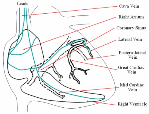
This technique can benefit Cardiac Resynchronization Therapy (CRT), which is aimed at the restoration of contractile coordination in hearts with severe heart failure (HF), sinus rhythm and ventricular conduction delay [11]. In 1998, a solution for multisite pacing using a transvenous technique has been proposed in [12]. Multisite pacing is achieved by stimulating both the right and left ventricles, pacing them simultaneously or with a small delay. The overall procedure consists in positioning endocardial leads in the right atrium and the right ventricle (RV) through the vena cava,
while the left ventricle (LV) is paced via a lead passed through the coronary sinus to an epicardial vein on the free wall of the left ventricle (Fig. 1).
The implant success rate is limited 85-92% by the difficulty of accessing the target vein for lead placement, incorrect or suboptimal pacing site selection and possible electrode displacements. The LV lead is therefore more challenging to implant than the RV one due to the difficulty in accessing some pacing sites and the risk of dissecting the coronary sinus. Currently, no planning procedure is performed and the interventions are only intra-operatively guided by conventional X-ray angiography. Multislice Computed Tomography (MSCT) with rendering can be used for CRT planning.
The objective of our present work is thus to assist physicians in planning the implant procedure. Our work relies on the study of a patient’s coronary anatomy to define the target vein, find the best path to reach it, confirm its accessibility and minimize the implant time. As introduced above, this percutaneous technique involves placing a lead at an appropriate location going from the cava vein, through the right atrium, the coronary sinus, the great vein to a posterolateral or a lateral vein.
The anatomical structures to be explored have different features. The heart cavities are large but enhanced by a contrast medium (typically not uniformly distributed) and the veins, which are small, divide in branches. The densities of the enhanced blood in the cavities and the walls partially overlap, which leads to false boundary detection, particularly regions enhanced by the contrast medium and looking like “particles” of different sizes occluding the walls and the entrance of the coronary sinus. A new algorithmic extension to improve the detection of the walls and, at the same time, remove these enhanced regions, is described in section 2. Results are then presented and discussed with a few examples in section 3.
2. Rendering method
The algorithm to improve the visualization into the cavities relies on a detection of objects during the volume traversal and a discrimination by their size, small regions being associated to artifacts due to the non-uniform distribution of contrast medium, large regions corresponding to the endocardial walls. The general framework described in [13] (without any pre-processing of the raw
volume) is based on rays cast from the observer to the volume data through the screen pixels and is carried out as follows:
- a progression mode that involves incrementing the position along the ray: this increment must be small enough to avoid unexpected crossings of surfaces and, therefore, missing their detection.
- rough detection using simple (e.g. thresholding) or more complex operators (like moment-based [14])
- a refinement step which consists of linearly interpolating the area where the surface has been approximately detected and performing more precise detection by decreasing the increment. This interpolation can deal with non-uniform sampling of slices or lead to a better spatial resolution (classically up to 1/5 voxel). The local gradient maximum is then searched and the surface orientation is computed for shading.
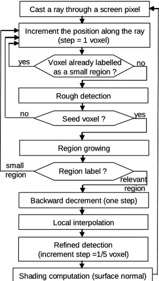
The present algorithm shown Fig. 2 is based on the same detection and interpolation steps. However, it adds a region growing stage during ray casting. It operates as follows: each time an “object” is detected by thresholding along a ray, i.e. when the voxel value is less than the contrast threshold (CT), a local region growing algorithm is launched with the reference voxel serving as a seed point. The neighborhood of this voxel is then analyzed and all connected voxels satisfying the threshold condition (voxel value < CT) are stored in a stack and counted, marked as visited. This is done until the stack is no longer increasing or a certain stopping criterion is met. This criterion is the size threshold (ST). This parameter determines the maximum size (in the number of voxels) of the “particle-like” regions that should be filtered out. If the detected region size is smaller than ST, the corresponding object is considered as an artifact and the ray-casting process using the rough detection scheme is continued by omitting the small “particle” found.
When a region is large enough (relevant region), the ray traversal is stopped and the first detected voxel is assumed to be a point on the surface of interest (e.g. the endocardial wall). A 3-D linear interpolation is performed in the neighborhood (i.e. from the eight voxels surrounding the considered point), and more refined detection is initiated as described above.
3. Results and discussion
This new algorithm has been implemented on a PC workstation and applied to 8 angio-MSCT acquired on a Siemens Somatom volume zoom, with 4 detectors. The identical protocol was used with the following acquisition parameters: collimation of 0.6 mm, table displacement of 1.5 mm/rotation, slice thickness of 1.25 mm, reconstruction increment of 0.6 mm, size of the matrix 512x512 with about 200 slices and a voxel size from 0.33x0.33x0.33 to 0.4x0.4x0.4 mm3 after interpolation of the reconstructed data set. The contrast resolution is 12 bits.
A qualitative evaluation of the algorithm has been first conducted by two interventional cardiologists. The locations of the virtual sensor were varied in the right atrium and ventricle, the only cavities of concern here to reach the coronary sinus. The two parameters (contrast and size) that influence the results in terms of detection of walls and elimination of the artifacts were varied and their effects were evaluated. Although there is a trade-off between the two parameters (the contrast and size thresholds are not independent in this case), we have found that they can be selected from a rather wide range of values (from 40 to 120 Hounsfield Units and 1000 to 1500 voxels respectively) while facilitating the search of the coronary sinus. The selection of thresholds can be carried out during an interactive session. Three orthogonal views are displayed in order to locate a sensor and its orientation. In Fig. 3, the 3-D images are computed without (standard ray casting with detection and local interpolation) and with the region growing algorithm, and they show that the “particle-like” artifacts are effectively removed while the inner surface of the heart cavities remains well defined.
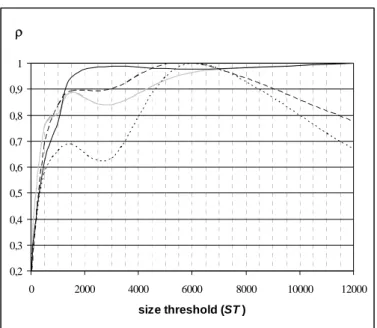
A quantitative study has then been carried out to estimate the features (number, size) of the regions that are eliminated with different parameter values. The region features do not vary linearly with the two parameters. They depend very much on the image data set and on the non-uniform distribution of the contrast medium as well as the selected locations and viewpoints. Therefore, relevant statistics, measuring the effectiveness of the method and defining the best parameter setting, are difficult to establish. The number of eliminated regions can vary from 10 to 300 but is on average lower in the atrium (around 100) than in the ventricle (around 150) due to the difference in their volumes. The mean size of these regions can vary from 60-100 to 120-200 voxels when CT is increased from 40 to 120 HU (100 voxels representing about 3.6 or 6.4 mm3 depending of the volume resolution). Fig. 4 illustrates the relative mean size of eliminated regions with respect to CT and ST. Let MS(CT, ST) be the mean size of the eliminated regions, and MMS(CT) be the maximum of MS(CT,
ST) over the range considered for ST when CT is fixed. Fig. 4 shows the relative size of the eliminated
regions, ρ(CT, ST) = MS(CT, ST)/MMS (CT), for four different values of CT (40 HU, 70 HU, 100 HU,
120 HU) when ST is varied from 30 to 12000 voxels. For CT = {40 HU, 70 HU}, the mean size of the eliminated regions is less than 100 voxels. It is interesting to note that for CT = 70 HU ρ is always greater than 95 % when ST > 1500 voxels. For CT = {100 HU, 120 HU}, the mean size of the eliminated regions reaches values higher than 120 voxels. These results indicate that in the case of a too high value of CT, the sizes of the occluding regions are too large and can be connected to the walls: they do not anymore look like “particle-like” regions, i.e. rather small isolated regions.
Since the major objective of this study is to help the physician in achieving the access to the left venous tree, the visual inspection, as illustrated by Fig. 3, is important. Other solutions to view the main structures of interest during the navigation have been examined (for instance by undersampling the volume). No improvements were obtained and, moreover, local features of the surface cavities were lost. The present algorithm and the pre-operative navigation have several advantages: (i) no prior segmentation is required; (ii) the visibility of the walls is improved and helps the physician in finding the coronary sinus, the first step in accessing the venous coronary tree; (iii) additional measurements (distance to the coronary sinus, angle to enter into it, and size of a catheter to be used) can be performed during the navigation that can be used by the physicians before an operation. The fact that no pre-segmentation is carried out has, of course, a disadvantage in that it increases the computational requirements. Using a PC with a 2-GHz CPU and 1-GB memory, it takes on average 3 seconds (with
ST = 1500 voxels) for the exploration of the ventricles, twice the time required when no region
growing is performed. The computation time increases with ST. A more intensive clinical evaluation is in progress but it already appears that a full planning session will not last more than 10 minutes. However, the overall benefit in terms of intra-operative time saving and efficiency has still to be evaluated.
4. Conclusion
A new algorithm has been proposed to filter out “particle-like” objects in 3-D volumes rendered using ray casting methods. It relies on a region growing scheme with only two control parameters. It has been applied to cardiac MSCT to improve the viewing of heart cavities during navigation with the
objective of locating the coronary sinus with ease. The evaluation conducted so far has shown that the visual perception of the structures of interest is improved. This work is a step toward the definition of optimal left ventricular pacing.
Acknowledgements
The authors are indebted to the anonymous reviewers for their many helpful comments and corrections. This work was supported by a grant from the French Ministry of Research (CIT 04T187).
References
[1] H. Hauser, L. Mroz, G.I. Bischi, M.E. Gröller, “Two-Level Volume Rendering,” IEEE
Transactions on Visualization and Computer Graphics, vol. 7, no. 3, pp. 242-252, 2001.
[2] M. Meißner, J. Huang, D. Bartz, K. Mueller, R. Crawfis, "A Practical Evaluation of Four Popular Volume Rendering Algorithms," in Proc. ACM Symposium on Volume Visualization, Salt Lake City, pp. 81-90, 2000.
[3] W.E. Lorensen, H.E. Cline, “Marching cubes: a high resolution 3-D surface construction algorithm,” Computer Graphics, vol. 21, no. 3, pp. 163-169, 1987.
[4] M. Levoy, “Display of Surfaces from Volume Data,” IEEE Computer Graphics and
Applications, vol. 9, pp. 29-36, 1988.
[5] J. Udupa, G.T. Herman, 3D Imaging in Medicine. CRC Press,1991.
[6] A.E. Kaufman, S. Lakare, K. Kreeger, I. Bitter, “Virtual Colonoscopy,” Communications of the
ACM, vol. 48, no. 2, pp. 37-41, 2005.
[7] R.A. Robb, “Virtual endoscopy: development and evaluation using the Visible Human datasets,”
Computerized Medical Imaging & Graphics, vol. 24, no. 3, pp. 133-151, 2000.
[8] D. Bartz, Ö. Gürvit, M. Lanzendörfer, A. Kopp, A. Küttner, W. Straßer, "Virtual Endoscopy for Cardio Vascular Exploration," in Proc. Computer Aided Radiology and Surgery (CARS 2001), Berlin, Germany, pp. 1005-1009, 2001.
[9] P. Haigron, G. Le Berre, J.L. Coatrieux, “3-D navigation in medicine,” IEEE Engineering in
Medicine and Biology, vol. 15, no. 2, pp. 70-78, 1996.
[10] P. Haigron, M.E. Bellemare, O. Acosta, C. Goksu, C. Kulik, K. Rioual, A. Lucas, “Depth-Map-Based Scene Analysis for Active Navigation in Virtual Angioscopy,” IEEE Transactions on
Medical Imaging, vol. 23, no. 11, pp. 1380-1390, 2004.
[11] C. Leclercq, D.A. Kass, “Re-timing the failing heart: principles and current clinical status of cardiac resynchronization,” Journal of the American College of Cardiology, vol. 39, pp. 194-201, 2002.
[12] J. Daubert, P. Pitter, H. Le Breton, D. Gras, C. Leclercq, A. Lazarus, J. Mugica, P. Mabo, S. Cazeau, “Permanent left ventricular pacing with transvenous leads inserted into the coronary veins,” PACE , vol. 21, pp. 239-245, 1998.
[13] J.L. Dillenseger, C. Hamitouche, J.L. Coatrieux, “Visualisation d’images tridimensionnelles par lancer de rayon avec interpolation locale,” Innovation et Technologie en Biologie et Médecine, vol. 12, no. 3, pp. 244-255, 1991.
[14] L.M. Luo, C. Hamitouche, J.L. Dillenseger, J.L. Coatrieux, “A moment-based three-dimensional edge operator,” IEEE Transactions on Biomedical Engineering, vol. 40, no. 7, pp. 693-703, 1993.
List of figures
Fig. 1. Lead paths in transvenous biventricular pacing.
Fig. 2. Flowchart of ray casting.
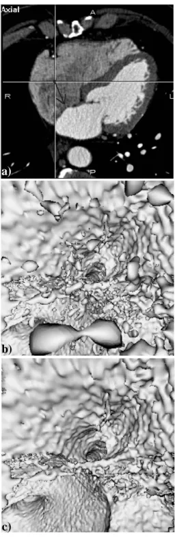
Fig. 3. Inside the right atrium. (a) Axial MSCT slice showing the location and the orientation of the virtual sensor (dark arrow) located in the right atrium and looking towards the entrance of the coronary sinus. (b) Virtual endoscopy image computed without region growing (CT = 70 HU). The artifact regions to be eliminated appear like isolated particles in suspension within the atrium cavity. (c) Virtual endoscopy image computed with region growing (CT = 70 HU, ST = 1500 voxels). The entrance of the coronary sinus (at the centre of the image) and the surrounding endocardial wall (top half of the image) are clearly visible.
Fig. 4. Evolution of the relative mean size ρ = MS (CT, ST) / MMS (CT) of the eliminated regions for different values of size threshold ST and contrast threshold CT. MS(CT, ST) is the mean size of the eliminated regions, and MMS(CT) is the maximum of MS(CT, ST) over the range considered for ST when CT is fixed.
Fig. 1. Lead paths in transvenous biventricular pacing.
Cast a ray through a screen pixel Increment the position along the ray
(step = 1 voxel)
Seed voxel ?
Region label ?
Backward decrement (one step) Local interpolation
Refined detection (increment step =1/5 voxel) Shading computation (surface normal)
no yes
small region
relevant region Voxel already labelled
as a small region ?
no yes
Region growing Rough detection
Fig. 2. Flowchart of ray casting.
a) c) b) a) c) b)
Fig. 3. Inside the right atrium. (a) Axial MSCT slice showing the location and the orientation of the virtual sensor (dark arrow) located in the right atrium and looking towards the entrance of the coronary sinus. (b) Virtual endoscopy image computed without region growing (CT = 70 HU). The artefact regions to be eliminated appear like isolated particles in suspension within the atrium cavity. (c) Virtual endoscopy image computed with region growing (CT = 70 HU, ST = 1500 voxels). The entrance of the coronary sinus (at the centre of the image) and the surrounding endocardial wall (top half of the image) are clearly visible.
ρ 0,2 0,3 0,4 0,5 0,6 0,7 0,8 0,9 1 0 2000 4000 6000 8000 10000 12000 size threshold (ST ) CT = 40 HU ; MMS = 79 voxels CT = 70 HU ; MMS = 97 voxels CT = 100 HU ; MMS = 134 voxels CT = 120 HU ; MMS = 126 voxels
Fig. 4. Evolution of the relative mean size ρ = MS (CT, ST) / MMS (CT) of the eliminated regions for different values of size threshold ST and contrast threshold CT. MS(CT, ST) is the mean size of the eliminated regions, and MMS(CT) is the maximum of MS(CT, ST) over the range considered for ST when CT is fixed.