HAL Id: hal-00174498
https://hal.archives-ouvertes.fr/hal-00174498
Preprint submitted on 25 Sep 2007
HAL is a multi-disciplinary open access
archive for the deposit and dissemination of
sci-entific research documents, whether they are
pub-lished or not. The documents may come from
teaching and research institutions in France or
L’archive ouverte pluridisciplinaire HAL, est
destinée au dépôt et à la diffusion de documents
scientifiques de niveau recherche, publiés ou non,
émanant des établissements d’enseignement et de
recherche français ou étrangers, des laboratoires
Fast tensor-product solvers: Part II: Spectral
discretization in space and time.
Yvon Maday, Einar M Rønquist
To cite this version:
Yvon Maday, Einar M Rønquist. Fast tensor-product solvers: Part II: Spectral discretization in space
and time.. 2007. �hal-00174498�
Fast tensor-product solvers:
Part II: Spectral discretization in space and time
Yvon Maday
∗, and Einar M. Rønquist
†July 23, 2007
Abstract
We consider the numerical solution of an unsteady convection-diffusion equation using high order polynomial approximations both in space and time. General boundary conditions and initial conditions can be imposed. The method is fully implicit and enjoys exponential convergence in time and space for analytic solutions. This is confirmed by numerical ex-periments (in one space dimension) using a spectral element approach in time and a pure spectral method in space. A fast tensor-product solver has been developed to solve the coupled system of algebraic equations for the O(Nd
) unknown nodal values within a single space-time spectral element. This solver has a fixed complexity of O(Nd+1
) floating point operations and a memory requirement of O(Nd
) floating point numbers. An alternative solution method, allowing for a parallel implementation and more easily extendable to more complex problems is sketched out at the end of the paper.
1
Introduction
There have been a number of research efforts in the past with the goal of using high order approximations both in time and space for the numerical solution of time-dependent partial differential equations. The first contribution we are aware of was done more than 25 years ago [7, 8], while the most recent work we have found on this topic is within the last few months [13, 9]. While the use of high order (spectral) approximations in space is currently a well developed field, the same is not true for the time direction. Encouraging progress has been made over the past couple of decades [11, 12, 1, 10, 13, 9], however, a significant advance, appropriate for solving real applications, is still missing.
From a pure approximation point of view, the motivation for using high order approximations in time is at least as strong as for using such methods in space. Indeed, for many problems the regularity in time is at least as high as the regularity in space. For parabolic problems, there may exist singularities at t = 0, however, this situation is simpler to analyze than the various spatial singularities resulting from the presence of vertices, edges and faces. Furthermore, while the solution may exhibit sharp boundary layers in space, this may often not be the case in the time direction. Of course, there may be problems where the regularity of the solution with respect to time can be expected to be low; nonetheless, the motivation for using high order approximations in time is quite significant.
∗Universit´e Pierre et Marie Curie-Paris6, UMR 7598, Laboratoire J.-L. Lions, Paris, F-75005 France and
Division of Applied Mathematics, Brown University, 182 George Street, Providence, RI 02912, USA
†Norwegian University of Science and Technology, Department of Mathematical Sciences, N-7491 Trondheim,
What has prevented the adoption of high order methods in time has fundamentally been related to computational complexity. In general, such an approach will result in implicit systems of algebraic equations. If the number of degrees-of-freedom in space is already large, multiply-ing this number with a large factor in the time direction poses significant challenges in terms of solver technology. Unless the computational cost for the solvers is close to optimal, i.e., the cost is approximately proportional with respect to the number of degrees-of-freedom (a condition partially alleviated when high order approximations are used), the method will not be competi-tive with a more conventional time-advancing discretization based on low order finite difference approximations where the solution is advanced one small time step at a time.
There are a number of reasons for revisiting the approach used for the temporal treatment. First, the computers are now becoming quite powerful with many (thousands of) processors and with a large aggregate memory. Second, there have recently been several alternative methods proposed to exploit more parallelism in the time direction [1, 6]. Third, a number of fast solution algorithms are currently available, and some of these may be exploited with respect to the time direction [2].
In this paper, we first consider the numerical discretization of the time-dependent convection-diffusion equation in one space dimension based on high order polynomial approximations in time and space. For simplicity, we assume a polynomial approximation of degree N in each direction. We then develop a fast tensor-product solver for the resulting system of algebraic equations; this solver can be classified as a direct solver. We also present numerical results demonstrating the convergence properties of the method.
We will discuss the extension to multiple space dimensions and nonlinear problems in a future paper. The focus of this paper is the use of spectral elements in time, and exploring the possibilities of exploiting the tensor-product feature between space and time in order to construct fast solution algorithms.
2
The heat equation
For the sake of simplicity, let us consider first the one-dimensional heat equation ∂u
∂t = κ ∂2u
∂x2 + f (x, t) in ωx= (0, L), (1) subject to the homogeneous boundary conditions
u(x = 0, t) = 0, ∀ t ∈ ωt= [0, T ], u(x = L, t) = 0, ∀ t ∈ ωt,
(2) and subject to the initial condition
u(x, t = 0) = s(x). (3)
Here, u(x, t) is the solution (the temperature), κ is the thermal diffusivity, and f (x, t) is a thermal heat source that depends on space and time. We assume that the thermal diffusivity, κ, is a constant.
A common approach when discretizing this equation is to discretize space and time separately. In particular, when applying a spectral discretization, it is common to only consider a spectral discretization in space; discretization in time is typically done using a multi-stage method or a multi-step method [4, 5].
2.1
Weak formulation
We consider here a spectral discretization in both space and time. The discretization will be based upon a weak space time formulation of the problem: Find u ∈ X such that
Z T 0 Z L 0 ∂u ∂t v dx dt = −κ Z T 0 Z L 0 ∂u ∂x ∂v ∂xdx dt + Z T 0 Z L 0 f v dx dt, ∀v ∈ X0. (4) with X = H1(ωt, L2(ωx)) ∩ L2(ωt, H01(ωx)) and e.g. X0= {w ∈ X, w(x, 0) = 0}, together with the initial condition u(x, 0) = s(x) satisfied over ωx.
This is similar to a standard variational procedure, except for the fact that we here integrate the governing equation over both space and time.
Next, we consider the (space-time) domain
Ω = (0, L) × (0, T ) = ωx× ωt as an affine mapping of the reference domain
Φ : bΩ = (−1, 1) × (−1, 1) −→ Ω.
In the following, we denote a point in the reference domain as (ξ, η), and use the convention that a “hat” refers to a quantity defined in terms of the reference variables, e.g.,
ˆ
u = u ◦ Φ.
The weak formulation can then be expressed in the reference variables as: Find ˆu ∈ bX such that Z ˆ Ω ∂ ˆu ∂ηv dξ dη + γˆ 1 Z ˆ Ω ∂ ˆu ∂ξ ∂ˆv ∂ξdξ dη = γ2 Z ˆ Ω ˆ f ˆv dξ dη, ∀ˆv ∈ bX0, (5) where b X = { ˆw, w ◦ Φˆ −1∈ X}, Xb0= { ˆw, w ◦ Φˆ −1∈ X0}, and γ1= 2 κ T L2, γ2= T 2.
2.2
A spectral discretization in space and time
We now consider a spectral discretization of the continuous problem (5) in space and time. In particular, we consider a discretization based on high-order polynomials. We define our discrete spaces as
b
where PN(bΩ) is the space of all functions which are polynomials of degree less than or equal to N in each direction ξ and η. The Galerkin approximation of (5) is : Find ˆuN ∈ bXN such that
Z ˆ Ω ∂ ˆuN ∂η vˆNdξ dη + γ1 Z ˆ Ω ∂ ˆuN ∂ξ ∂ˆvN ∂ξ dξ dη = γ2 Z ˆ Ω ˆ f ˆvNdξ dη, ∀ˆvN ∈ bXN0, (6) In order to represent an element in the linear space bX0
N, we choose a tensor-product, La-grangian interpolant basis through the Gauss-Lobatto Legendre (GLL) points, ξi, i = 0, . . . , N . Specifically, ∀ˆvN ∈ bXN0, we write ˆ vN(ξ, η) = N X i=0 N X j=0 vijℓi(ξ) ℓj(η), (7) where vij = ˆvN(ξi, ξj) = vN(x(ξi), y(ξj)). The Lagrangian interpolants satisfy the properties
ℓk(ξ) ∈ PN(ˆω), ∀ k ∈ {0, . . . , N }, ℓk(ξl) = δkl, ∀ k, l ∈ {0, . . . , N }2.
(8) Note that some of the basis coefficients in (7) are explicitly imposed by the boundary condi-tions and the intial condition. In particular, vi0= 0 for i = 0, ..., N , v0j= 0 for j = 0, ..., N , and vN j= 0 for j = 0, ..., N .
The discrete solution ˆuN will be an element of bXN. Similar to (7), we express the discrete solution in the reference variables as
ˆ uN(ξ, η) = N X m=0 N X n=0 umnℓm(ξ) ℓn(η). (9) The following basis coefficients are given by the boundary conditions: u0n= 0 for n = 0, . . . , N , and uN n = 0 for n = 0, . . . , N . The initial condition is given by setting um0 = sm = s(x(ξm)) for m = 0, . . . , N . Hence, the initial condition is approximated by the N th order polynomial interpolant through the GLL points. Approximating the given heat source f also as a high order interpolant, the discrete problem can be expressed as: Find ˆuN ∈ bXN such that
Z 1 −1 Z 1 −1 [ N X m=0 N X n=0 umnℓm(ξ) ℓn′(η) ] ℓi(ξ) ℓj(η) dξ dη+ γ1 Z 1 −1 Z 1 −1 [ N X m=0 N X n=0 umnℓm′ (ξ) ℓn(η) ] ℓi′(ξ) ℓj(η) dξ dη = γ2 Z 1 −1 Z 1 −1 [ N X m=0 N X n=0 fmnℓm(ξ) ℓn(η) ] ℓi(ξ) ℓj(η) dξ dη , ∀i ∈ {1, . . . , N − 1}, ∀j ∈ {1, . . . , N }. (10)
We have here chosen ˆvN to be ℓi(ξ) ℓj(η) for all i ∈ {1, . . . , N − 1}, and for all j ∈ {1, . . . , N }. This will give us enough equations to determine the unknown basis coefficients umn for all m ∈ {1, . . . , N − 1}, and for all n ∈ {1, . . . , N }.
If we introduce the notation that, ∀v, w ∈ L2(−1, 1), (v, w) =
Z 1 −1
we can also write the discrete problem (10) as: Find ˆuN ∈ bXN such that N X m=0 N X n=0 (ℓi, ℓm) (ℓj, ℓn′) umn+ γ1 N X m=0 N X n=0 (ℓ′ i, ℓm′ ) (ℓj, ℓn) umn= γ2 N X m=0 N X n=0 (ℓi, ℓm) (ℓj, ℓn) fmn ∀i ∈ {1, . . . , N − 1}, ∀j ∈ {1, . . . , N }. (12)
The final step in the discretization process is to evaluate (or approximate) the L2 innerprod-ucts (·, ·) with numerical quadrature. A common and natural choice is to use Gauss-Lobatto Legendre (GLL) quadrature, e.g.,
(v, w) = Z 1 −1 v(ξ) w(ξ) dξ ≈ N X α=0 ραv(ξα) w(ξα) ≡ (v, w)G. (13) Here, {ρα}Nα=0 and {ξα}Nα=0 are the GLL weights and points, respectively, and (·, ·)G represents the discrete L2 innerproduct. We recall that the GLL quadrature is exact for all integrands in
P2N −1(−1, 1).
We now introduce the one-dimensional mass matrix bB with elements b
Bkl = (ℓk, ℓl)G = ρkδkl, (14) the one-dimensional convection matrix bC with elements
b
Ckl = (ℓk, ℓl′)G = ρkDkl, (15) and the one-dimensional stiffness matrix bA with elements
b Akl= (ℓk′, ℓl′)G = N X α=0 ραDαkDαl. (16)
Here, we have introduced the derivative matrix
Dαk≡ ℓk′(ξα). (17)
We remark that the mass matrix is diagonal, while the discrete innerproducts defining the con-vection matrix and the stiffness matrix are, in fact, exact.
The discrete problem, including quadrature, can thus be expressed as: Find ˆuN ∈ bXN such that, ∀i ∈ {1, . . . , N − 1}, ∀j ∈ {1, . . . , N }, N −1X m=1 N X n=1 ( bBimCbjn + γ1AbimBbjn ) umn= γ2 N −1X m=1 N X n=1 b BimBbjnfmn − N −1X m=1 δimCbj0sm. (18)
We remark that the last term on the right hand side represents the imposition of the initial condition via high order polynomial interpolation, with sm= s(x(ξm)).
Next, we define gij= γ2 N −1X m=1 N X n=1 b BimBbjnfmn − N −1X m=1 δimCbj0sm. (19) ∀i ∈ {1, . . . , N − 1}, ∀j ∈ {1, . . . , N }; this expression incorporates all the known data for this problem, including the initial condition.
Once we have computed gij, we can write the algebraic problem as: Find ˆuN ∈ bXN such that, ∀i ∈ {1, . . . , N − 1}, ∀j ∈ {1, . . . , N }, N −1X m=1 N X n=1 ( bBimCbjn + γ1AbimBbjn) umn= gij. (20) Instead of representing the unknown basis coefficients umn as a multidimensional array (i.e., with one, local index for each direction ξ and η, we can, of course, also represent the unknown basis coefficients as a single, long vector u; the associated local-to-global mapping is done by using the convention that the first index (i.e., along ξ) “runs faster” than the second index (i.e., along η). Note that u = R(N −1)N.
We can then write the system (20) using tensor-product forms: Find u = R(N −1)N such that ( bC2⊗ bB1 + γ1Bb2⊗ bA1 ) u = g. (21) Here, g is the global vector corresponding to the multi-dimensional array gij, bC is the one-dimensional convection operator defined in (15), bA is the one-dimensional diffusion operator defined in (16), and bB is the one-dimensional mass matrix defined in (14). Note that we use subscript 1 and 2 to differentiate between the directions ξ and η, respectively. For example,
b
B1 and bA1are square matrices of size (N − 1) × (N − 1), corresponding to Dirichlet boundary conditions at the end points ξ = ±1. In contrast, bB2and bC2are square matrices of size N × N , corresponding to Dirichlet boundary conditions at η = −1.
Our objective now is to develop a fast tensor-product solver for (21). To this end, we need to diagonalize the operators. First, we solve the generalized eigenvalue problem
b
A1Q1= bB1Q1Λ1
associated with direction 1, i.e., ξ (or space). Here, Q1 is the eigenvector matrix, and Λ1 is a diagonal matrix containing the eigenvalues. Since bA1 and bB1 are both symmetric and positive definite, all the eigenvalues are real and positive, and the eigenvectors are ortogonal with respect to the mass matrix bB1. In fact, if we normalize the eigenvectors so that
QT
1 Bb1Q1= I1,
we see that
QT1 Ab1Q1= Λ1. Hence, we can express bA1 and bB1 in (21) as
b A1= Q−T 1 Λ1Q−11 , b B1= Q−T1 Q−11 . (22)
Second, we would like to diagonalize the convection operator bC2 with respect to the mass matrix bB2, i.e., we consider the eigenvalue problem
b
C2S2= bB2S2Λ2, (23) where S is a matrix containing the eigenvectors as columns. Now, since Dirichlet conditions are only specified at η = −1, the convection operator bC2 is not skew-symmetric and therefore not normal. Hence, at a fundamental level, we do not know whether we are able to diagonalize bC2. Even if we can diagonalize bC2, the eigenvectors will certainly not be orthogonal with respect to the mass matrix, and this fact can cause numerical difficulties. However, as discussed in [3], we expect to be able to diagonalize bC2 for N ≤ 32 without any significant round-off errors. This limitation on N should not pose any major constraint since we do not (at least currently) forsee using a too high value of N in the time direction.
In the following, we therefore assume that we are in this regime, i.e., N ≤ 32. The eigenvalues and eigenvectors are complex, and we can express bC2 and bB2 in (21) as
b C2= bB2S2Λ2S−1 2 , b B2= bB2S2S−12 . (24)
Substituting for bB1, bA1, bC2 and bB2in (21) and using the usual rules for tensor products, the system (21) can be expressed as
( bB2S2⊗ Q−T
1 )( Λ2⊗ I1 + γ1I2⊗ Λ1 )( S−12 ⊗ Q−11 ) u = g. (25) We thus see that that the solution u can be expressed explicitly as
u = ( S2⊗ Q1 )( Λ2⊗ I1 + γ1I2⊗ Λ1)−1( S−12 Bb −1
2 ⊗ QT1 ) g . (26) At this point, several comments are in order. First, we have demonstrated that it is possible to develop a fast, direct solver for the problem at hand, at least for a polynomial approximation N ≤ 32 in the time direction. Second, the expression (26) will not be used directly in its cur-rent form. Indeed, we will revert back to a multi-dimensional array representation, and perform the necessary operations using matrix-matrix products. This will give an overall computational complexity of O(N3). In contrast, if we explicitly form the global matrices, the computational complexity would be O(N4). In higher space dimensions, the difference between these two ap-proaches will be much higher. For example, it is possible to extend the methodology presented here to two and three space dimensions when the domain is tensorized. With three space dimen-sions and one time dimension, the complexity of the solver will be O(N5) for O(N4) unknowns (assuming for simplicity that we use the same polynomial degree in each spatial direction as well as in the time direction for each spectral element in time). Finally, note that the solution we arrive at represents a fully implicit, high-order polynomial approximation (high order in both space and time).
3
The unsteady convection-diffusion equation
We now consider the one-dimensional, unsteady convection-diffusion equation ∂u ∂t + ∂u ∂x = κ ∂2u ∂x2 + f (x, t) in ωx= (0, L), (27)
subject to the same boundary conditions and initial condition as before.
In terms of discretization, we follow an identical approach as for the heat equation. We thus arrive at the discrete problem: Find ˆuN ∈ bXN such that
( bC2⊗ bB1 + β bB2⊗ bC1 + γ1Bb2⊗ bA1) u = g. (28) where bC1 is the usual convection operator in space, bB2 is the mass matrix associated with the time direction, and the constant β = T
L. Note that bC1 is a matrix of size (N − 1) × (N − 1), while bC2is a matrix of size N × N . Furthermore, bC1 is a skew-symmetric matrix (for the given boundary conditions), while bC2 is not.
In the following, our objective is to develop a fast, tensor product solver for (28); we now present two alternatives for achieving this.
3.1
Alternative 1
Similar to the unsteady heat equation, we again rely on being able to solve the eigenvalue problem (23) associated with the time direction. We recall that a fundamental issue here is the fact that the matrix bC2 is not normal, and that the eigenvalue problem (23) may not have a solution. However, as discussed in [3], the eigenvalues and eigenvectors can be computed without any significant round-off errors for N ≤ 32.
For the space direction, we propose to solve the following eigenvalue problem:
(β bC1+ γ1Ab1) S1= bB1S1Λ1. (29) This allows us to write
(β bC1+ γ1Ab1) = bB1S1Λ1S−11 , b
B1= bB1S1S−11 .
(30) Using the above information, the system (28) can be then expressed as
( bB2S2⊗ bB1S1)( Λ2⊗ I1 + I2⊗ Λ1 )( S−12 ⊗ S−11 ) u = g. (31) We thus see that that the solution u can be expressed explicitly as
u = ( S2⊗ S1 )( Λ2⊗ I1 + I2⊗ Λ1 )−1( S−12 Bb −1
2 ⊗ S−11 Bb
−1
1 ) g. (32)
For efficiency reasons, a local numbering scheme should be used to represent the right hand side as well as the solution.
This alternative thus relies on being able to solve the eigenvalue problem (29) in addition to the eigenvalue problem (23). However, since the discrete convection-diffusion operator in (29) is not normal either, (29) may not have a solution even if we have not experienced any numerical difficulty so far; see the numerical experiments reported in the next section.
3.2
Alternative 2
This alternative, which we shall develop further in Part III of the series, only relies on diagonal-izing the first order operator in the time direction. Combining (24) and (28), and using the rules for tensor-products, we end up with
Introducing the variables ˜ u = ( S−1 2 ⊗ I1 ) u, (34) ˜ g = ( S−1 2 Bb −1 2 ⊗ I1 ) g, (35) we can express (33) as ( Λ2⊗ bB1 + I2⊗ (β bC1+ γ1Ab1)) ˜u = ˜g. (36) Reverting back to the local numbering scheme, we can alternatively write (36) as
N −1X
m=1
[(γ1Ab1+ β bC1)im+ λj( bB1)im] ˜umj= ˜gij, i = 1, . . . N − 1, j = 1, . . . , N. (37) For each value of j, we solve a steady convection-diffusion-type system. Each of these systems is of dimension N − 1. In the linear case, the N systems we end up with can be solved com-pletely independently. This is similar to the approach presented in [2], but here involving a non-symmetric operator instead of a symmetric one. Once the solution ˜u has been computed, we can find u via the transformation (34); in practice, we compute this transformation using a local numbering scheme; see [2].
4
Numerical results
We consider here the unsteady convection-diffusion equation (27) in ωx = (0, 1) (i.e., L = 1), with an exact solution
u(x, t) = sin(πt) sin(πx).
We apply the proposed discretization scheme and integrate the discrete equations until a final time Tfinal = 40 corresponding to 20 full periods in time. The time interval is split up into K equal subintervals of size T . The tensor-product solver (32) is then used to solve the system of algebraic equations associated with each space-time spectral element.
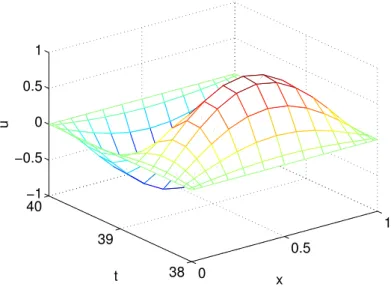
We first use a time step (or spectral element size in time) equal to T = 2, corresponding to one full period in time. The numerical solution corresponding to the last time interval is shown in Figure 1.
Note that, with this choice of time step (T = 2), the initial condition for each time interval corresponds to a homogeneous condition. This is by no means necessary. In Figure 2, we again show the numerical solution corresponding to the last time interval, but now choosing a smaller time step T = 4/3 (independent of the period of the solution); with this choice it takes K = 30 time steps to arrive at the same final time Tfinal= 40.
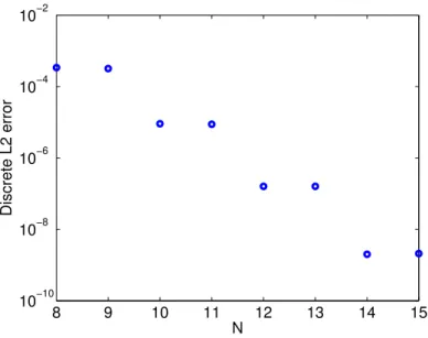
Finally, we measure the error in the discrete L2 norm as a function of the polynomial degree N for a fixed time step T = 2. The error is measured over the last time interval (i.e., the last space-time spectral element), and the convergence results are reported in Figure 3. As expected, exponential convergence is achieved. Note that the odd values of N do not give any reduction in the error; this is due to the fact that the solution is even with respect to both space and time over each whole period in time.
5
Conclusions
For a one dimensional example, we have presented a method for solving the linear convection-diffusion equation using high order polynomial approximations in both time and space. General boundary conditions and initial conditions can be imposed. The method is fully implicit and enjoys exponential convergence in time and space for analytic solutions. This is confirmed by numerical experiments using a spectral element approach in time and a pure spectral method in space (in one space dimension).
A fast tensor-product solver has been developed to solve the coupled system of algebraic equations for the O(Nd) unknown nodal values within a single space-time spectral element. For simplicity, we have here assumed a polynomial approximation of degree N in each direction. This solver has a fixed complexity of O(Nd+1) floating point operations and a memory requirement of O(Nd) floating point numbers. The polynomial approximation in the time direction should be chosen to be less than or equal to 32 in order to avoid any round-off errors.
6
Future work
Future work will focus on solving more complex time-dependent partial differential equations (multiple space dimensions; linear and nonlinear equations). For example, the proposed methods could be interesting to use for the approximation of the time-dependent Maxwell equations.
In the case of the unsteady convection-diffusion equations, the extension to multiple space dimensions will be based on a similar approach as presented in [2] in the context of solving elliptic problems in partially deformed three-dimensional domains. In particular, we will exploit the tensor-product representation that always exists between the single time direction and the (generally deformed) physical domain. This will always allow us to achieve parallelism through the solution of independent steady convection-diffusion-type problems as in Alternative 2.
0 0.5 1 38 39 40 −1 −0.5 0 0.5 1 x t u
Figure 1: The numerical solution computed at the last time interval, i.e., for 38 ≤ t ≤ 40 (∆T = 2). The polynomial degree in both the spatial and temporal direction is N = 15. The error in the discrete L2 norm is 2.1 · 10−9.
0 0.5 1 38.5 39 39.5 40 −1 −0.5 0 0.5 1 x t u
Figure 2: The numerical solution computed at the last time interval, i.e., for 38.6666 ≤ t ≤ 40 (T = 4/3). The polynomial degree in both the spatial and temporal direction is N = 15. The error in the discrete L2 norm is 3.6 · 10−12.
8 9 10 11 12 13 14 15 10−10 10−8 10−6 10−4 10−2 N Discrete L2 error
Figure 3: Convergence results for the convection-diffusion problem. The size of each spectral element in the time direction is T = 2.
References
[1] Bar-Yoseph, P., Moses, E., Zrahia, U., and Yarin, A. (1995). Space-time spectral element methods for one-dimensional nonlinear advection-diffusion problems. J. Comput. Phys., 119, 62-74.
[2] Bjøntegaard, T., Maday, Y., and Rønquist, E.M. (submitted, 2007). Fast tensor-product solvers. Part I: Partially deformed three-dimensional domains.
[3] Canuto, C., Hussaini, M.Y., Quarteroni, A., and Zang, T.A. (2006). Spectral Methods, Springer-Verlag.
[4] C.W. Gear (1971). Numerical Initial Value Problems in Ordinary Differential Equations, Prentice-Hall.
[5] E. Hairer, S.P. Nørsett and G. Wanner (1993). Solving Ordinary Differential Equations I, Springer.
[6] Lions, J.-L., Maday, Y., and Turninici, G. (2001). R´esolution d’EDP par un sch´ema en temps parar´eel. C.R. Acad Sci. Paris S´er. I Math., 332, 661-668.
[7] Morchoisne, Y. (1981). Pseudo-spectral space-time calculations of incompressible viscous flows. AIAA Paper, No. 81-0109.
[8] Morchoisne, Y. (1984). Inhomogeneous flow calculations by spectral methods: Mono-domain and multi-domain techniques. In Voigt, R.G, Gottlieb, D., and Hussaini, M.Y. (eds.) Spectral Methods for Partial Differential Equations, SIAM, Philadelphia.
[9] Shen, J. and Wang, L.-L. (2007). Fourierization of the Legendre-Galerkin method and a new space-time spectral method. Appl. Numer. Math., 57, 710-720.
[10] Shukla, P. and Eswaran, V. (1996). A fully spectral method for hyperbolic equations. Int. J. Numer. Meth. Engrg., 39, 67-79.
[11] Tal-Ezer, H. (1986). Spectral methods in time for hyperbolic problems. SIAM J. Numer. Anal., 23, 11-26.
[12] Tal-Ezer, H. (1989). Spectral methods in time for parabolic problems. SIAM J. Numer. Anal., 26, 1-11.
[13] Tang, J.-G. and Ma, H.-P. (2007). A Legendre spectral method in time for first-order hy-perbolic equations. Appl. Numer. Math., 57, 1-11.