HAL Id: inserm-00978660
https://www.hal.inserm.fr/inserm-00978660
Submitted on 14 Apr 2014
HAL is a multi-disciplinary open access
archive for the deposit and dissemination of
sci-entific research documents, whether they are
pub-lished or not. The documents may come from
teaching and research institutions in France or
abroad, or from public or private research centers.
L’archive ouverte pluridisciplinaire HAL, est
destinée au dépôt et à la diffusion de documents
scientifiques de niveau recherche, publiés ou non,
émanant des établissements d’enseignement et de
recherche français ou étrangers, des laboratoires
publics ou privés.
Powers of the likelihood ratio test and the correlation
test using empirical bayes estimates for various
shrinkages in population pharmacokinetics.
François Combes, Sylvie Retout, Nicolas Frey, France Mentré
To cite this version:
François Combes, Sylvie Retout, Nicolas Frey, France Mentré. Powers of the likelihood ratio test
and the correlation test using empirical bayes estimates for various shrinkages in population
phar-macokinetics..
CPT: Pharmacometrics and Systems Pharmacology, American Society for
Clini-cal Pharmacology and Therapeutics ; International Society of Pharmacometrics, 2014, 3, pp.e109.
�10.1038/psp.2014.5�. �inserm-00978660�
Population pharmacokinetics (PK) is increasingly used in drug development and is based on nonlinear mixed-effect models (NLMEMs).1 Several software algorithms developed to estimate the parameters of these models have been compared, as by Plan et al.2 The first and most popular software is NONMEM and, since version 7, several estima-tion algorithms have been available, such as first-order con-ditional estimation with interaction (FOCEI) and stochastic approximation expectation maximization (SAEM). Gibian-sky et al.3 compared the performance of NONMEM estima-tion methods in simulated examples of a target-mediated drug disposition model using either default options or by designing the options to get the best possible results for each algorithm (“expert” options). They demonstrated the importance of the estimation options in the algorithm per-formance by comparing standard errors of NONMEM esti-mates with those predicted using PFIM 3.2 optimal design software.4 The SAEM algorithm provided estimates similar to those of FOCEI.
For a given model, when population parameters are esti-mated, individual parameters from individual observations can be estimated by a Bayesian approach using the maximum
a posteriori method. If the data are from the individuals used to estimate population parameters, the same approach is used, but it is an empirical Bayes estimation. These individual parameter estimates are useful for investigating the influence of the individual’s baseline characteristics on the individual parameters.5
Population analysis allows the use of sparse sampling, but the sampling design influences the precision of popula-tion estimates.6 The informativeness of a data set in param-eter estimation is a function of the number of subjects and of the number and timing of the samples.7 Optimal design methodology allows determination of the most informative
design with constraints. It computes a criterion, such as the D-optimality criterion, from the Fisher information matrix (MF), which depends on the structural model, the parameter values, and the design.8
Thus, the design also greatly influences the precision of empirical Bayes estimates (EBEs). For a rich design, the a
posteriori distributions of the individual random effects are centered on the true values with small standard deviations. When little information is available for each individual (sparse design), the means of these distributions regress towards the population mean with larger SDs. A formula from lin-ear mixed-effect methodology has been used to predict this shrinkage of EBEs associated with a design.9 This shrinkage should be evaluated before conducting a clinical trial. Using a simulation study, we provide here a good prediction of shrink-age using the Bayesian Fisher information matrix (MBF)9,10, avoiding the use of extensive simulations.
In a study of the impact of shrinkage on model building, Savic and Karlsson11 show that covariate relationships may be masked or falsely induced and that the shape of the true relationship may be distorted when examined using a test of the correlation between the EBEs and the covariates. Savic and Karlsson11 recommend as follows: “When shrinkage is high, other diagnostics and more direct population model estimation need to be employed in model building and evalu-ation.” They suggest more extensive use of the likelihood ratio test (LRT) test for covariate evaluation and selection when shrinkage is large, which is much more time consuming than selection from EBEs.
However, to our knowledge, no one has compared the power of LRT with the power of the correlation test (CT) with respect to design selection and its expected shrinkage. We therefore compared type 1 errors and power in detecting the effect of a continuous covariate using either the LRT or the
Received 13 November 2013; accepted 20 January 2014; published online 9 April 2014. doi:10.1038/psp.2014.5
We compared the powers of the likelihood ratio test (LRT) and the Pearson correlation test (CT) from empirical Bayes estimates
(EBEs) for various designs and shrinkages in the context of nonlinear mixed-effect modeling. Clinical trial simulation was
performed with a simple pharmacokinetic model with various weight (WT) effects on volume (V). Data sets were analyzed with
NONMEM 7.2 using first-order conditional estimation with interaction and stochastic approximation expectation maximization
algorithms. The powers of LRT and CT in detecting the link between individual WT and V or clearance were computed to explore
hidden or induced correlations, respectively. Although the different designs and variabilities could be related to the large
shrinkage of the EBEs, type 1 errors and powers were similar in LRT and CT in all cases. Power was mostly influenced by
covariate effect size and, to a lesser extent, by the informativeness of the design. Further studies with more models are needed.
CPT Pharmacometrics Syst. Pharmacol. (2014) 3, e109; doi:
10.1038/psp.2014.5
; published online 9 April 2014
1IAME UMR 1137, INSERM, Paris, France; 2IAME UMR 1137, Université Paris Diderot, Sorbonne Paris Cité, Paris, France; 3Institut Roche de Recherche et Médecine
Translationnelle, Boulogne-Billancourt, France; 4Pharma Research and Early Development, Clinical Pharmacology, F. Hoffmann-La Roche Ltd, Basel, Switzerland.
Correspondence: FP Combes (francois.combes@inserm.fr)
Powers of the Likelihood Ratio Test and the Correlation
Test Using Empirical Bayes Estimates for Various
Shrinkages in Population Pharmacokinetics
FP Combes1,2,3,4, S Retout3,4, N Frey4 and F Mentré1,2
CPT: Pharmacometrics & Systems Pharmacology
Power of LRT and CT for Various Shrinkages in PK
Combes et al. 2
CT based on EBEs according to various designs, along with various associated shrinkages.
Through an extensive Monte–Carlo simulation of a simple one-compartment PK model, we compared the performances of FOCEI and SAEM algorithms before evaluating the type 1 errors and powers of the tests to detect covariate influences on individual parameters. We also created several scenarios to vary the informativeness of the PK design and therefore the associated shrinkage.
RESULTS
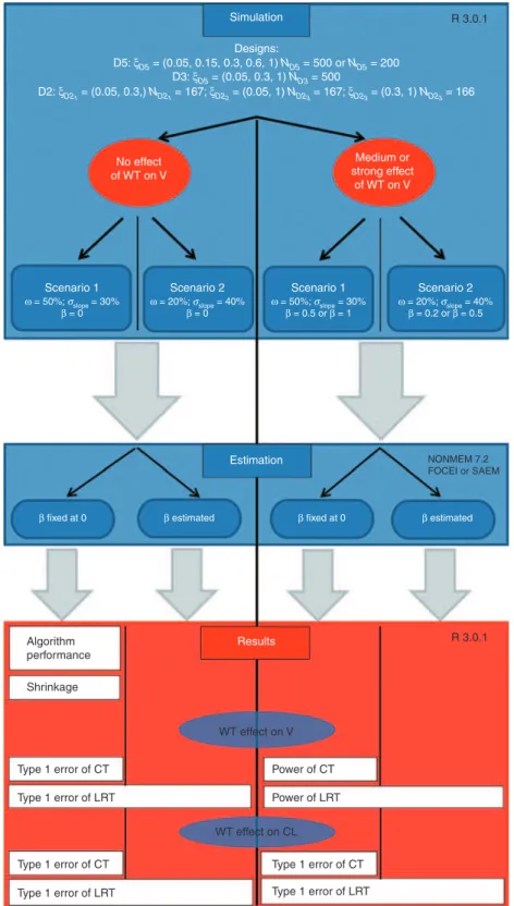
Figure 1 summarizes the different clinical trial simulations performed.
Algorithm performance
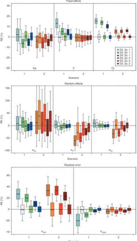
Figure 2 presents, for each scenario and each design with
N = 500, the boxplots of relative errors on parameters esti-mated using either FOCEI or SAEM with NONMEM 7.2. SAEM always provided more accurate estimates than FOCEI, except for ωka in scenario 2. Estimates with the FOCEI algo-rithm were often slightly biased, mainly for volume (V), clear-ance (CL), ωV, and ωCL, and for residual error parameters. Bias was more marked for designs D2 and D3. Median val-ues of relative errors using SAEM were less influenced by the design and were always close to 0%.
Considering that SAEM gave more accurate esti-mates than FOCEI, only SAEM power estiesti-mates are pre-sented below. FOCEI power estimates are available in the Supplementary Materials online.
Prediction of shrinkage
Figure 3 shows predicted shrinkage vs. boxplots of observed shrinkage on V (left) and CL (right) for each design and each scenario without covariate effect. The simulated sce-narios generated predicted shrinkage values that increased from D5 to D2. Confirming previous results,9 M
BF gave a good prediction of observed shrinkage. The boxplots were closely centered on the identity line, with small deviations for low shrinkages, for which there was a trend to predict lower shrinkages (but by less than or around 10% from median val-ues of observed shrinkage).
Evaluation of tests
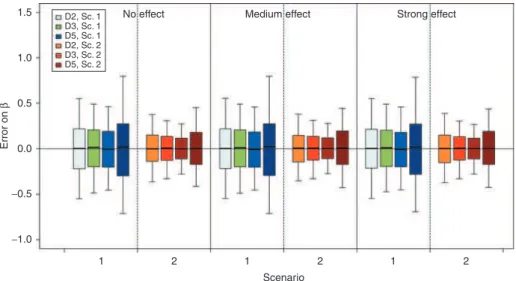
Figure 4 presents the boxplot of the error on β estimates for each scenario, design, and covariate effect. The covari-ate effect was always correctly estimcovari-ated. When comparing the effect of the total number of subjects, the boxplots clearly show an increase in the SD of estimates with decrease in number of subjects.
Type 1 errors and the powers of tests between weight (WT) and V are presented in Table 1 for all scenarios and designs and are illustrated in Figure 5. Type 1 error was similar for LRT and CT, even for high values of shrinkage, and in all cases, it was within the prediction interval of 3.65–6.35%. The power of LRT was equal to the power of CT in all scenarios, even with high shrinkage, the greatest difference being 2% for D5 with 200 subjects in scenario 1. Figure 5a illustrates how LRT and CT have very similar type 1 error and power.
The power was 95% for scenario 1 and 86% for scenario 2, with rich designs and a strong effect of WT. Figure 5b shows the lack of trend between shrinkage and power across sce-narios and covariate effects. As expected, the power of tests was directly linked to the covariate effect. For both scenarios, a design modification led to a 25% increase in power when, for a given scenario and design, a change in covariate effect size induced a 50% increase.
When comparing N = 500 with D2 and N = 200 with D5, both with the same total number of samples, power was higher for D2 with a similar type 1 error.
When the covariate effect on CL was explored, type 1 error was similar for LRT and CT in all cases (Table 1). When no covariate effect was simulated on V, type 1 error remained within the range of the prediction interval, around 5%. Sur-prisingly, this type 1 error increased with the β value, espe-cially in scenario 2. Type 1 errors were in all cases around 5% in scenario 1, except for D3 with β = 0.5 (N = 500, 6.4% for LRT) and for D5 with β = 1 (N = 500, 6.6% for CT). Consider-ing scenario 2, the type 1 error computed for a strong covari-ate effect led to a significant increase in the type 1 error, for D2 (8.7% for LRT and 8.2% for CT), D3 (9.7% for CT and 9.6% for LRT), and D5 (N = 500, 6.9% for LRT). In this sce-nario, the increase in type 1 error is linked to higher corre-lation between individual V and CL. The median correcorre-lation was −0.25 for D2 and −0.23 for D3. Median correlation was −0.13 for scenario 2, D5, whereas for scenario 1, almost no correlation in the EBEs was found.
DISCUSSION
We have compared, for different scenarios and different PK sampling designs leading to various amounts of shrinkage, the type 1 error and power of two tests to detect the effect of a continuous covariate on a PK parameter: the LRT, which compares the log-likelihoods of two nested models; and a correlation test between the covariate and the EBEs.
Surprisingly, both tests showed the same power irrespec-tive of the scenario or the design considered. Indeed, even if LRT is based on the fitting of two models to get the two likelihoods, it did not show greater power than a simple CT based on EBEs, even with high shrinkage. As a conclusion, because of its faster execution, we think that the CT should be used in a first screening of the relevant covariates, and then the selected covariates can be tested in a stepwise pro-cedure to build the full covariate model using the LRT.
Savic and Karlsson11 highlighted a possible issue when using the CT to screen covariates when there is high shrink-age in the EBEs and recommended a test that does not rely on EBEs. Our study shows that such a test, the LRT for instance, does not behave differently from the CT, what-ever the shrinkage. Indeed, the loss of power associated with high shrinkage in CT has the same influence in the LRT and is linked with less information in the design. It also showed that the size of the covariate effect is the main factor linked to any covariate detection issue. Bertrand et al.12 showed a similar link between power and covariate effect. To a lesser extent, the information in the design also has an impact on the power, which decreases when the number of sampling
times per subject decreases. Furthermore, when comparing the two designs with the same number of samples, power was found to be greater for 500 subjects (D2) than for 200 (D5), though the latter has lower shrinkage (Table 1, with β = 1, with WT effect on V). This decrease in power for 200 sub-jects can be explained by the very challenging conditions we
used to simulate the covariate effect (rather small variance of WT and rather small covariate effect). These results are in accordance with the loss of power associated with decreased number of subjects reported by Liu et al.13 and Bertrand et al.14 Nevertheless, even if the LRT was not significant, the covariate effect, β, was always correctly estimated.
Figure 1 Global scheme of the clinical trial simulations. CL, clearance; CT, correlation test; FOCEI, first-order conditional estimation with interaction; LRT, likelihood ratio test; SAEM, stochastic approximation expectation maximization; V, volume; WT, weight.
Simulation Designs: D5: ξD5 = (0.05, 0.15, 0.3, 0.6, 1) ND5 = 500 or ND5 = 200 D2: ξD21 = (0.05, 0.3,) ND21 = 167; ξD22 = (0.05, 1) ND23 = 167; ξD23 = (0.3, 1) ND23 = 166 No effect of WT on V Medium or strong effect of WT on V Scenario 1 ω = 50%; σslope = 30% β = 0
β fixed at 0 β estimated β fixed at 0 β estimated
Scenario 2 ω = 20%; σslope = 40% β = 0 Scenario 1 Estimation Results R 3.0.1 R 3.0.1 WT effect on V WT effect on CL Power of CT Power of LRT Type 1 error of CT Type 1 error of LRT Type 1 error of CT Algorithm performance Shrinkage Type 1 error of LRT Type 1 error of CT Type 1 error of LRT NONMEM 7.2 FOCEI or SAEM ω = 50%; σslope = 30% β = 0.5 or β = 1 Scenario 2 ω = 20%; σslope = 40% β = 0.2 or β = 0.5 D3: ξD5 = (0.05, 0.3, 1) ND3 = 500
CPT: Pharmacometrics & Systems Pharmacology
Power of LRT and CT for Various Shrinkages in PK
Combes et al. 4
Considering the induction of correlation due to high shrinkage, a slight inflation of type 1 error in scenario 2 was found. This inflation could be explained by the EBE corre-lation between V and CL. The influence of design on EBE
correlation should be investigated in future work. Further work is also needed to explore the influence of design on a full covariate modeling process, with several covariates influ-encing the parameters.
Figure 2 Boxplot of relative error (RE; %) on estimated fixed effects (top) without covariate effect, random effects (middle), and residual error parameters (bottom) according to scenario 1 or 2, the design, and the estimation algorithms. Boxplots represent the median, quartiles, and 5–95% percentiles. Colors stand for the design and the scenario. For the same color, the dark areas represent the first-order conditional estimation with interaction algorithm and the pale areas denote the stochastic approximation expectation maximization algorithm. Sc., scenario.
1 1 Ka ωKa σ inter σslope ω V ωCL −30 −100 −50 0 50 RE (%) −10 −20 0 20 40 60 RE (%) 100 150 −20 −10 0 RE (%) 10 20 30 V CL 2 2 Scenario Random effects Fixed effects 1 2 1 1 2 2 Scenario Residual error 1 1 2 2 Scenario 1 2 D2, Sc. 1 D2, Sc. 1 D5, Sc. 1 D2, Sc. 2 D2, Sc. 2 D5, Sc. 2
This simulation study also confirms the good prediction of shrinkage using the Bayesian Fisher information matrix, as already shown in ref. 9, when planning clinical studies. This could be helpful in the design of population studies wherein individual estimation of individual parameters with small shrinkage is needed.
As expected, our investigations showed that the SAEM algorithm reliably and accurately estimates population parameters, even for sparse designs. FOCEI gave surpris-ingly biased results for such a simple model even with rather informative designs. This bias could be explained by the rather large residual error used in our simulations, inducing bias in the linearization during FOCEI.15 This result is not unusual considering previous comparisons of FOCEI and SAEM for continuous data. Girard and Mentré reported that methods without likelihood approximations, such as SAEM (using a version that later became MONOLIX (MOdèles NOn LInéaires à effets miXtes)) perform better than first order or FOCEI.16 Using a previous version of NONMEM (5 and 6β), Dartois et al.17 reported very good estimation of parameters despite some discrepancies in residual error estimates and
recommended the use of exact methods such as SAEM instead of FOCEI. At the time of these two studies, SAEM was not implemented in NONMEM. In addition, Ueckert et
al.18 and Johannson et al.19 showed the same loss of “robust-ness” and “precision” of FOCEI compared with SAEM, for continuous data, especially when mu-modeling is used for SAEM in NONMEM 7. Finally, Plan et al.2 compared vari-ous algorithms using NONMEM, Statistical Analysis System, MONOLIX, and R and found that FOCEI was in some cases more biased than SAEM, especially for sparse designs, along with issues related to the convergence of the algorithm.
Results for the power of CT and LRT for data sets analyzed using the FOCEI algorithm can be found in the Supplementary Materials online for designs D2 and D5 with N = 500 subjects. Despite some rather biased estimations of population param-eters with FOCEI, there was no bias in the estimation of β. Type 1 error and power were similar for FOCEI and SAEM, with only a slight inflation of the type 1 error in scenario 2 for sparse designs. Our selection of the NONMEM 7.2 algorithm and options relied on advice and results presented in ref. 3. Further work is needed to explore the influence of the algorithm options (number of samples and iterations for Monte Carlo importance sampling (IMP) algorithm) on the likelihood computation.
Larger residual error variances than those used in our study may be rather unusual in the field of pharmacometrics. We performed our study for a wide range of shrinkages, and the tests performed similarly whether the generated shrink-age was low or high (Table 1). The use of different error mod-els and the magnitude of those errors could affect the amount of generated shrinkage.9,20 A high residual error would obvi-ously decrease the power of the test. Further work is needed on the extent to which similarities between CT and LRT are influenced by the level and form of residual error.
In our simulation study, we used a rather narrow distribution of covariates and challenging medium covariate effects. This was done on purpose because, for greater covariate distribu-tion and larger covariate effect, the power was very high and we could not investigate the influence of other factors. We studied covariate effects using a power function along with an exponential form of random effects. These forms are the most used in population PK modeling. Studies using other forms of random effects and covariate models are therefore needed.
We only explored the power of covariate detection using LRT and CT with different designs and variabilities. LRT and CT are still the most used in population PK. Future work should focus on other covariate selection methods, such as Generalized Additive Modeling (GAM) analysis21 and Least Absolute Shrinkage and Selection Operator (LASSO),22 but these are mainly used when several covariates are consid-ered. Furthermore, the impact of structural model misspecifi-cation could be evaluated along with the effect of design on the covariate selection process.23
The main objective of our work was to compare the perfor-mance of CT and LRT for different shrinkages. Although we used a rather simple model, the outcomes provided important information in line with the findings of Savic and Karlsson,11 and the screening of covariates was done with CT instead of the more time-consuming LRT. The next step will be to confirm our results with a more complex model, such as a target-mediated drug disposition model, which involves the use of differential
Figure 3 Predicted shrinkage (%) value vs. boxplot of observed shrinkage (%) with the stochastic approximation expectation maximiz ation algorithm for the 1,000 replicates without covariate effect, for parameters volume (V) and clearance (CL), each design, and scenarios 1 or 2. Colors stand for the design and the scenario. Sc., scenario. 0 0 20 40 Predicted shr inkage (%) 60 80 100 D2, Sc. 1 D3, Sc. 1 D5, Sc. 1 D2, Sc. 2 D3, Sc. 2 D5, Sc. 2 20 40 60 Observed shrinkage (%) 80 100 0 0 20 40 Predicted shr inkage (%) 60 80 100 20 40 60 Observed shrinkage (%) CL V 80 100
CPT: Pharmacometrics & Systems Pharmacology
Power of LRT and CT for Various Shrinkages in PK
Combes et al. 6
equations and for which use of CT should be all the more bene-ficial in a model development process, considering the runtime that such a system requires for parameter estimation.
METHODS
Models and notations
For a given individual, let yi be the vector of n observed con-centrations at n sampling times ξi = {ti,1,…,ti,n} for subject i and
f be the known function describing the PK model. So, yi was assumed to be modeled as follows:
yi=f
(
θ ,ξi i)
+εi(1) where θi is the p vector of individual PK parameters, θi = (θi,1,…,θi,p)T; ε
i is the random error, following a normal distri-bution with zero mean and variance Σ(θi, ξi). Here, Σ(θi, ξi) is defined as the variance matrix of a combined error model
with an additive component σinter and a proportional one σslope; hence, Σ(θi, ξi) = diag ((σinter + σslope f(θi, ξi))2).
Individual parameters θi are defined as θi = g(θ, ηi) where θ is the vector of p fixed effects and ηi is the vector of p individual random effects ηi = (ηi,1,…,ηi,p)T. Random effects ηi follow a normal distribution with zero mean and variance Ω. For Ω, a diagonal p × p matrix of variances of random effects Ω =diag(ω12,…,ωp2) was assumed. For g(θ,ηi), an exponential model, where g(θ η ) θ η
k, i,k = ek i,k was
consid-ered, k = {1,…,p}. The vector Ψ of population parameters is composed of
{
θ1,…, ,θ ωp 12,…,ω σp2, 2inter, σslope2}
.In PK modeling, population parameters are estimated by the method of maximum likelihood. Individual parameters are estimated by a Bayesian approach using the maximum
a posteriori as follows:
ˆ |
ηi=argmax
(
p(
ηi yi)
)
(2)Figure 4 Boxplot of error on the estimated β value with the stochastic approximation expectation maximization algorithm and for a covariate effect on volume (V), according to scenarios 1 or 2, the design, the simulated covariate effect value, and the number of subjects. Boxplots represent the median, quartiles, and 5–95% percentiles. Colors stand for the design and the scenario. For D5, pale and dark areas are used, respectively, for designs with 500 and 200 subjects. Sc., scenario.
No effect D2, Sc. 1 D3, Sc. 1 D5, Sc. 1 D2, Sc. 2 D3, Sc. 2 D5, Sc. 2 −1.0 −0.5 0.0 1 2 1 2 Scenario 1 2 0.5 Error on β 1.0
1.5 Medium effect Strong effect
Table 1 Type 1 error (%, β = 0), power (%, β ≠ 0) of LRT and CT tests for covariate effect, and predicted shrinkage on V and CL for all scenarios, simulated
covariate effect levels, and designs
n N Test WT on V WT on CL Scenario 1 ω = 50%; σslope = 30% Scenario 2 ω = 20%; σslope = 40% Scenario 1 ω = 50%; σslope = 30% Scenario 2 ω = 20%; σslope = 40% Predicted shrinkage Power (%) Predicted shrinkage Power (%) Predicted shrinkage Power (%) Predicted shrinkage Power (%) β β β β 0 0.5 1 0 0.2 0.5 0 0.5 1 0 0.2 0.5 2 500 LRT 56 3.8 29.7 84.8 84 4.2 14.3 59.4 43 4.7 4.6 4.6 85 5.5 6.2 8.7 CT 3.9 29 83.6 4.0 14.3 60.1 4.5 4.5 4.5 4.8 5.8 8.2 3 500 LRT 37 4.6 38.3 91.6 78 4.6 18.6 76.2 22 5.8 6.4 6.3 69 5.6 6.8 9.6 CT 4.3 37.7 90.6 4.9 18.0 75.2 6.1 6.1 6.3 5.4 6.1 9.7 5 500 LRT 31 4.8 43.5 95.4 72 5.0 25.0 85.7 14 6.1 5.6 5.8 59 4.8 4.7 6.9 CT 4.7 43.4 93.9 5.0 24.0 84.8 6.0 5.8 6.6 4.3 4.9 6.3 5 200 LRT 31 5.7 20.5 64.1 72 4.7 11.7 47.7 14 5.6 5.3 5.0 59 5.2 5.3 6.1 CT 5.9 19.6 62.1 4.8 11.6 47.4 5.1 5.2 5.2 5.0 4.9 5.6
Population parameters were estimated using the SAEM algorithm. Type 1 errors outside the prediction interval are written in bold.
where p(ηi|yi) is the probability distribution of ηi given yi, which can be expressed using the Bayes theorem as shown below: p y p y p p y ηi i η η i i i | | .
(
)
=(
) ( )
( )
(3)To estimate ηˆi by maximum a posteriori is equivalent to
minimizing, with respect to ηi:
− ×2
(
ln(
p y(
i| ηi)
)
+ln(
p( )
ηi)
)
(4) This is equal to j n y f g t f g t =∑
−(
(
)
)
(
)
+(
(
)
)
(
)
1 i,j i i,j 2inter slope i i,j
, , , , θ η
σ σ θ η 22
inter slope i i,j
i ln , +
(
+(
(
)
)
)
+ =∑
σ σ θ η η f g t k p , 2 1 ,,k k 2 2 ω . (5)PK model of the simulation study
A simulated example involving a one-compartment model with a single oral administration was used. The three param-eters are the absorption rate (ka), the apparent volume of distribution (V), and the apparent clearance (CL). For a given dose D, the prediction at time ti,j is shown below:
f t D ka V ka V V t ka t θi i,j i i i i i CL CL e e i i i,j i i,j ,
(
)
= × × − − − × − × (6)We chose θka = 10, θV = 0.2, and θCL = 0.5 with a dose D = 1. As this model is theoretical, we did not consider any specific units. The PK profile for these typical values of parameters is shown in Figure 6. To explore the influence of shrinkage in various situations, two scenarios were considered: for sce-nario 1, ω = 50% for each parameter and σslope = 30%;, for scenario 2, ω = 20% and σslope = 40%. Σinter was set to 0.15 in both cases, which is small with respect to the range of con-centrations covered by the PK model (see Figure 6 for the mean concentration–time course profile).
Study design
N = 500 subjects were simulated using three designs. First, a design with five samples (D5) per subject, ξD5 = {0.05, 0.15. 0.3, 0.6, 1}, was simulated and is presented in Figure 6. The simulation code is provided in the Supple-mentary Materials online. For these sampling times, the most informative design with three samples (D3) was then determined using a D-optimality approach: ξD2 = (0.05,0.3,1}. Finally, from ξD3, a two-sample design (D2) with three groups of one-third of the N subjects each was cre-ated: ξD21= {0 05 0 3. , . } (ND21= 167 subjects), ξD22 ={ .0 05 1, }
(ND22= 167 subjects), and ξD23={0.3, 1} (ND23 =166
subjects). Design D5 was also evaluated with N = 200 subjects, which corresponds to the same total number of observations as D2 with 500 subjects.
Evaluation of estimation
In the first step, R = 1,000 data sets were simulated without covariate effect for each design (D2, D3, and D5 with N = 500) and each scenario. Each data set was analyzed using NONMEM 7.224 with FOCEI and with SAEM to explore algo-rithm performances. Expert options inspired by Gibiansky et
al.3 were used for the setting of the SAEM algorithm (INTER-ACTION NBURN=15000 ISAMPLE=3 NITER=5000 SIGL=8 CTYPE=3 CINTERVAL=100). NONMEM codes are available in the Supplementary Materials online. Rela-tive errors of estimations of population parameters, (in per-centage), were computed for each component as in Eq. 7:
Figure 5 Power of likelihood ratio test (LRT) between weight (WT) and volume (V) (%), for all scenarios and designs (estimation with stochastic approximation expectation maximization algorithm) vs. (a) correlation test (CT; %; the black line represents the identity line). (b) Observed shrinkage on V (%) and covariate effect. Colors stand for the design and the scenario. Covariate effect is expressed by the background and colors: no effect with a colored line around dots, medium effect with fully colored dots, and strong covariate effect with black line around a colored dot. For D5, pale and dark areas are used respectively for designs with 500 and 200 subjects. Sc., scenario.
0 0 20 40 Po wer of LR T (%) 60 80 100 D2, Sc. 1 D3, Sc. 1 D5, Sc. 1 D2, Sc. 2 D3, Sc. 2 D5, Sc. 2 0 No effect Medium Covariate effect Strong100 80 60 Obser ved shr inkage (%) 40 20 20 40 Po wer of LR T (%) 60 80 100 20 40 60 Power of CT (%) 80 100
a
b
CPT: Pharmacometrics & Systems Pharmacology
Power of LRT and CT for Various Shrinkages in PK
Combes et al. 8 REr,k r,k k k =ψˆ −ψ × ψ 100 (7)
where ψˆr,k is the kth component of the vector of the
esti-mated population parameter for the rth data set and ψ
k is the
value used in the simulation. Prediction of shrinkage
As in the study by Combes et al.,9 the predicted shrinkage is computed as I−W(ξ) where
W I M
I
ξ ξ
( )
−( )
− −=
and is the identity matrix such that
BF 1 1 Ω , , :: I W−
( )
=M( )
− − ξ BF ξ 1 1 Ω (8)MBF can be approximated by a first-order linearization of the model25: M H FT T F H BF
( )
ξ =(
θ ξ,)
(
θ ξ,)
(
θ ξ,)
+ ∞ − − Σ 1 Ω 1 (9)where H = diag(θ1,…,θp) and F θ ξ f θ ξT θ , ( )
(
)
=∂ ∂ , . As Ω is diagonal, the diagonal elements of I−W, given in the Eq. 8, represent the ratio of the predicted variance of estimation using a Bayesian estimation and the a priori variance. When MBF−1 isclose to Ω (no information for the individual), I−W is close to I. In that case, shrinkage is expected to be high, close to 100%.
The selected designs and scenarios were chosen to lead to a wide range of predicted shrinkages on V and CL, between 31 and 84% for volume and between 14 to 85% for clearance (see results in Table 1).
For each data set r, the observed shrinkage of each com-ponent k was computed as follows:
Shk,r var k,r k,r = −
(
ˆ)
× ˆ 1 2η 100 ω (10)The distribution of the 1,000 observed shrinkages from the 1,000 data sets was compared with the predicted shrinkage. Evaluation of tests for covariate detection
We then considered a covariate model describing the influ-ence of the weight (WT) on volume using a power function:
θ θ β η V,i V i WT e WT V,i = (11)
We assumed a log-normal distribution of WT with a median
WT= 70 kg and a coefficient of variation of 10% (quantiles 2.5–97.5%: 57–85 kg). We considered this distribution range so as to avoid a very large distribution, which would contribute to very powerful covariate detection whatever the test and design. Designs involving 500 subjects led to powers close to 100% for LRT and CT, whatever the number of samples per individual.
R = 1,000 data sets for each design and scenario were simulated. For scenario 1, we first considered a case close to an allometric effect with β = 1. We then considered a smaller value of that effect β = 0.5 (medium effect) and no effect β = 0. Regarding scenario 2, as smaller variances were considered, we reduced the values of β to generate a strong covariate effect (β = 0.5), a medium effect (β = 0.2), or no effect (β = 0).
Using these simulations, we evaluated the properties of two tests in detecting the effect of the weight (WT) on volume (V). First, the LRT, which compares the log-likelihoods of the two nested models (with β fixed to 0 or β on V estimated), was con-sidered significant when the difference in −2 × log-likelihood was greater than 3.84, (the 95% limit of a χ2 distribution with one degree of freedom). The second test was a parametric correlation Pearson test between EBEs of volume from a pop-ulation analysis with no covariate in the model and weights.
Data sets were analyzed with the SAEM algorithm for population estimation. Likelihood was then computed by importance sampling (algorithm IMP in NONMEM 7.2 with 10 iterations and 3,000 samples).
We first estimated the covariate effect by exploring the error on the estimated β values as the estimated value of β minus the true value used for simulation.
Type 1 error α was then computed as the percentage of significant tests (P value < 0.05) in the R replicates simulated assuming a null hypothesis H0 (β = 0). We computed the 95% prediction interval for a binomial distribution with a probability of 0.05 and 1,000 replicates using the 2.5 and 97.5% per-centiles. The prediction interval was 3.65–6.35%. For a test with α = 0.05, we expect the estimated type 1 error to lie within this interval. The power of tests was computed as the percentage of significant tests in the R replicates simulated assuming the alternative hypothesis H1 (β ≠ 0).
Finally, in order to evaluate the risk of induction of covariate effects because of shrinkage,11 the same tests were evalu-ated for the relationship between WT and CL, although no WT effect was simulated in CL. We computed type 1 error for CT and LRT in the effect of WT on CL. Results (tests, predicted and observed shrinkage) were computed using R 3.0.1. Acknowledgments. During this work, the PhD of F.P.C. was sponsored by a Convention Industrielle de Formation par la Recherche from the French government and the Insti-tut Roche de Recherche et Médecine Translationnelle. The
Figure 6 Pharmacokinetic (PK) profile for the mean PK parameters of the simulated example with design D5.
0.0 0.0 0.2 0.4 0.6 Time 0.8 1.0 0.5 1.0 1.5 Concentration 2.0 2.5 3.0
authors thank IFR02 and Hervé Le Nagard for the use of the Centre de Biomodélisation.
Conflict of Interest. F.P.C. has a research grant from Roche and the French government. S.R and N.F work for F. Hoff-mann-La Roche Ltd, in Pharma Research and Early Devel-opment, Clinical Pharmacology. As an associate editor for
CPT: PSP, F.M. was not involved in the review or decision process for this manuscript.
Author Contributions. F.P.C., N.F., S.R., and F.M. designed the research. F.P.C. performed the research. F.P.C., S.R., and F.M. analyzed the results. F.P.C., S.R., N.F., and F.M. wrote the manuscript.
1. Pillai, G.C., Mentré, F. & Steimer, J.L. Non-linear mixed effects modeling - from methodology and software development to driving implementation in drug development science. J. Pharmacokinet. Pharmacodyn. 32, 161–183 (2005).
2. Plan, E.L., Maloney, A., Mentré, F., Karlsson, M.O. & Bertrand, J. Performance comparison of various maximum likelihood nonlinear mixed-effects estimation methods for dose-response models. AAPS J. 14, 420–432 (2012).
3. Gibiansky, L., Gibiansky, E. & Bauer, R. Comparison of Nonmem 7.2 estimation methods and parallel processing efficiency on a target-mediated drug disposition model.
J. Pharmacokinet. Pharmacodyn. 39, 17–35 (2012).
4. Bazzoli, C., Retout, S. & Mentré, F. Design evaluation and optimisation in multiple response nonlinear mixed effect models: PFIM 3.0. Comput. Methods Programs Biomed. 98, 55–65 (2010).
5. Bonate, P.L. Covariate detection in population pharmacokinetics using partially linear mixed effects models. Pharm. Res. 22, 541–549 (2005).
6. al-Banna, M.K., Kelman, A.W. & Whiting, B. Experimental design and efficient parameter estimation in population pharmacokinetics. J. Pharmacokinet. Biopharm. 18, 347–360 (1990).
7. Retout, S., Mentré, F. & Bruno, R. Fisher information matrix for non-linear mixed-effects models: evaluation and application for optimal design of enoxaparin population pharmacokinetics. Stat. Med. 21, 2623–2639 (2002).
8. Green, B. & Duffull, S.B. Prospective evaluation of a D-optimal designed population pharmacokinetic study. J. Pharmacokinet. Pharmacodyn. 30, 145–161 (2003). 9. Combes, F.P., Retout, S., Frey, N. & Mentré, F. Prediction of shrinkage of individual
parameters using the bayesian information matrix in non-linear mixed effect models with evaluation in pharmacokinetics. Pharm. Res. 30, 2355–2367 (2013).
10. Merlé, Y. & Mentré, F. Bayesian design criteria: computation, comparison, and application to a pharmacokinetic and a pharmacodynamic model. J. Pharmacokinet. Biopharm. 23, 101–125 (1995).
11. Savic, R.M. & Karlsson, M.O. Importance of shrinkage in empirical bayes estimates for diagnostics: problems and solutions. AAPS J. 11, 558–569 (2009).
12. Bertrand, J. & Balding, D.J. Multiple single nucleotide polymorphism analysis using penalized regression in nonlinear mixed-effect pharmacokinetic models. Pharmacogenet.
Genomics 23, 167–174 (2013).
13. Liu, M., Lu, W., Krogh, V., Hallmans, G., Clendenen, T.V. & Zeleniuch-Jacquotte, A. Estimation and selection of complex covariate effects in pooled nested case-control studies with heterogeneity. Biostatistics 14, 682–694 (2013).
14. Bertrand, J., Comets, E., Laffont, C.M., Chenel, M. & Mentré, F. Pharmacogenetics and population pharmacokinetics: impact of the design on three tests using the SAEM algorithm. J. Pharmacokinet. Pharmacodyn. 36, 317–339 (2009).
15. Ge, Z., Bickel, P.J. & Rice, J.A. An approximate likelihood approach to nonlinear mixed effects models via spline approximation. Comput. Stat. Data An. 46, 747–776 (2004). 16. Girard, P. & Mentré, F. A comparison of estimation methods in nonlinear mixed effects
models using a blind analysis. PAGE (Population Approach Group in Europe) 14. 16–17 June 2005, Pamplona, Spain.
17. Dartois, C., Lemenuel-Diot, A., Laveille, C., Tranchand, B., Tod, M. & Girard, P. Evaluation of uncertainty parameters estimated by different population PK software and methods.
J. Pharmacokinet. Pharmacodyn. 34, 289–311 (2007).
18. Ueckert, S., Johansson, A.M., Plan, E.L., Hooker, A. & Karlsson, M.O. New estimation methods in NONMEM 7: evaluation of robustness and runtimes. PAGE (Population Approach Group in Europe) 19. 8–11 June 2010, Berlin, Germany.
19. Johansson, A.M., Ueckert, S., Plan, E.L., Hooker, A. & Karlsson, M.O. New estimation methods in NONMEM 7: evaluation of bias and precision. PAGE (Population Approach Group in Europe) 19. 8–11 June 2010, Berlin, Germany.
20. Xu, X.S., Yuan, M., Karlsson, M.O., Dunne, A., Nandy, P. & Vermeulen, A. Shrinkage in nonlinear mixed-effects population models: quantification, influencing factors, and impact.
AAPS J. 14, 927–936 (2012).
21. Mandema, J.W., Verotta, D. & Sheiner, L.B. Building population pharmacokinetic– pharmacodynamic models. I. Models for covariate effects. J. Pharmacokinet. Biopharm. 20, 511–528 (1992).
22. Ribbing, J., Nyberg, J., Caster, O. & Jonsson, E.N. The lasso–a novel method for predictive covariate model building in nonlinear mixed effects models. J. Pharmacokinet.
Pharmacodyn. 34, 485–517 (2007).
23. Ribbing, J. & Jonsson, E.N. Power, selection bias and predictive performance of the Population Pharmacokinetic Covariate Model. J. Pharmacokinet. Pharmacodyn. 31, 109–134 (2004).
24. Beal, S., Sheiner, L.B., Boeckmann, A. & Bauer, R.J. NONMEM User’s Guides. (1989–2009), Icon Development Solutions, Ellicott City, Maryland, 2009.
25. Mentré, F., Burtin, P., Merlé, Y., Van Bree, J., Mallet, A. & Steimer, J.L. Sparse-sampling optimal designs in pharmacokinetics and toxicokinetics. Drug Inf. J. 29, 997–1019 (1995).
Study Highlights
WHAT IS THE CURRENT KNOWLEDGE ON THE TOPIC?
3
In population analysis, tests based on
correla-tion (CT) between empirical Bayes estimates
(EBEs) and covariates can be misleading when
those estimates are greatly shrunk. Tests
rely-ing on EBEs are therefore not recommended
for high shrinkage (Savic and Karlsson). There
is no study of the extent to which the loss of
power in the likelihood ratio test (LRT) is also
associated with sparser design.
WHAT QUESTION DID THIS STUDY ADDRESS?
3
This study compares the performances of the
LRT and the CT in detecting a continuous
covariate effect, according to different covariate
effect sizes and designs.
WHAT THIS STUDY ADDS TO OUR KNOWLEDGE
3
This study shows that for a simple PK model,
LRT and CT perform similarly, whatever the
covariate effect size and design, even in the
case of high shrinkage.
HOW THIS MIGHT CHANGE CLINICAL PHARMACOLOGY AND THERAPEUTICS
3
If the results are confirmed with more complex
models, CT should be used to screen
covari-ates, without any loss of power compared with
LRT and with a faster execution time.
CPT: Pharmacometrics & Systems Pharmacology is an open-access journal published by Nature Publishing Group. This work is licensed under a Creative Commons Attribution-NonCommercial-NoDerivative Works 3.0 License. To view a copy of this license, visit http://creativecommons.org/licenses/by-nc-nd/3.0/ Supplementary information accompanies this paper on the CPT: Pharmacometrics & Systems Pharmacology website