Deployment algorithms for multi-agent exploration and patrolling

Deployment Algorithms for Multi-Agent

HR

-

~.._7-..

Exploration and Patrolling

by

Mikhail Volkov

B.A., B.A.I., University of Dublin, Trinity College (2010)

Submitted to the Department of Electrical Engineering and Computer

Science

in partial fulfillment of the requirements for the degree of

Master of Science in Computer Science and Engineering

at the

MASSACHUSETTS INSTITUTE OF TECHNOLOGY

February 2013

©

Massachusetts Institute of Technology 2013. All rights reserved.

A u th or ...

Department of Electrical Engineering and Computer Science

January 28, 2013

C ertified by ... ...

...

Daniela Rus

Professor

Thesis Supervisor

Accepted by...

...

'&/

0

Cslie A. Kolodziejski

Chairman, Department Committee on Graduate Students

Deployment Algorithms for Multi-Agent

Exploration and Patrolling

by

Mikhail Volkov

B.A., B.A.I., University of Dublin, Trinity College (2010)

Submitted to the Department of Electrical Engineering and Computer Science on January 28, 2013, in partial fulfillment of the

requirements for the degree of

Master of Science in Computer Science and Engineering

Abstract

Exploration and patrolling are central themes in distributed robotics. These de-ployment scenarios have deep fundamental importance in robotics, beyond the most obvious direct applications, as they can be used to model a wider range of seemingly unrelated deployment objectives.

Deploying a group of robots, or any type of agent in general, to explore or patrol in dynamic or unknown environments presents us with some fundamental conceptual steps. Regardless of the problem domain or application, we are required to (a) under-stand the environment that the agents are being deployed in; (b) encode the task as a set of constraints and guarantees; and (c) derive an effective deployment strategy for the operation of the agents. This thesis presents a coherent treatment of these steps at the theoretical and practical level.

First, we address the problem of obtaining a concise description of a physical en-vironment for robotic exploration. Specifically, we aim to determine the number of robots required to be deployed to clear an environment using non-recontaminating exploration. We introduce the medial axis as a configuration space and derive a mathematical representation of a continuous environment that captures its under-lying topology and geometry. We show that this representation provides a concise description of arbitrary environments, and that reasoning about points in this rep-resentation is equivalent to reasoning about robots in physical space. We leverage this to derive a lower bound on the number of required pursuers. We provide a transformation from this continuous representation into a symbolic representation.

We then present a Markov-based model that captures a pickup and delivery (PDP) problem on a general graph. We present a mechanism by which a group of robots can be deployed to patrol the graph in order to fulfill specific service tasks. In particular, we examine the problem in the context of urban transportation, and establish a model that captures the operation of a fleet of taxis in response to incident customer arrivals throughout the city. We consider three different evaluation criteria: minimizing the

number of transportation resources for urban planning; minimizing fuel consumption

for the drivers; and minimizing customer waiting time to increase the overall quality

of service.

Finally, we present two deployment algorithms for multi-robot exploration and

patrolling. The first is a generalized pursuit-evasion algorithm. Given an

environ-ment we can compute how many pursuers we need, and generate an optimal pursuit

strategy that will guarantee the evaders are detected with the minimum number of

pursuers. We then present a practical patrolling policy for a general graph. We

evaluate our policy using real-world data, by comparing against the actual observed

redistribution of taxi drivers in Singapore. Through large-scale simulations we show

that our proposed deployment strategy is stable and improves substantially upon the

default unmanaged redistribution of taxi drivers in Singapore.

Thesis Supervisor: Daniela Rus

Title: Professor

Acknowledgments

Deus i fiel

Contents

1 Introduction

1.1 Motivations and Goals ...

1.2 Contributions to Robotics . . . .

1.3 Relation to Previous Work . . . .

1.4 Thesis Organization . . . .

2 Related Work

2.1 Exploration, Pursuit-Evasion and Patrolling

2.2 Applications to Urban Mobility . . . .

3 Environment Characterization for Non-Recontaminating 3.1 Problem Formulation . . . . 3.2 Environment Analysis . . . . 3.2.1 Environment Geometry . . . . 3.2.2 Exploration Model . . . . 3.3 Implementation . . . . 3.4 Sum m ary . . . . .

4 Deployment Algorithm for Non-Recontaminating Exploration

4.1 Topology Tree . . . .. . . . .

4.1.1 Exploration Rules ... 4.1.2 Environment Bounds ... 4.1.3 Optimal Pursuit Strategy ...

Exploration 12 12 18 20 22 23 23 24 26 27 30 30 32 39 42 43 44 45 47 51

. . . .

. . . .

4.2 Implementation ...

4.3 Summary . . . .

5 Markov-based Model for Future Urban

5.1 Problem Statement ...

5.2 Optimization Setup . . . .

5.2.1 Hastings-Metropolis Algorithm

5.3 Modeling Urban Mobility . . . .

5.3.1 Extended Network . . . .

5.3.2 Extended Redistribution Policy 5.3.3 Extended Stability Condition 5.4 Summary . . . .

6 Deployment Algorithm for Patrolling

6.1 Practical HM Policy . . . .

6.1.1

Accuracy and Complexity . .

6.2 Policy Criteria . . . .

6.3 Experiments . . . .

6.3.1

Results . . . .

6.4 Summary . . . .

7 Conclusions and Lessons Learned

Networks

Mobility

Urban

. . . . . . . .

an

Mobility Network

53

56

57

58

59

60

61

61

63

64

65

66

67

68

70

71

73

74

75

List of Figures

1-1 KOHGA3 and Quince search and rescue robots deployed in the after-math of the Tohoku Earthquake and Tsunami of 2011. . . . . 14 1-2 Aerial view of the Deepwater Horizon oil spill, 2010 (left) and the oil

absorbing robot deployed in the cleanup efforts (right). . . . . 15 1-3 A trivial example environment (left) and a more realistic non-trivial

environment (right). The free region is shown in white and the obstacle region is shown in black. . . . . 16

3-1 Fig. 3-1a shows a robot located at some position p within the free region

Q.

The sensor footprint H and its oriented boundary DH are shown on the right. Fig. 3-1b shows the inspected region It and the contaminated region Ut at some time t. Fig. 3-1c shows the inspected region boundary BI, the inspected obstacle boundary DIB and the frontier T . . . . 28 3-2 The environment is represented by a binary image in Fig. 3-2a. Fig.

3-2b shows the distance transform D of the environment. Fig. 3-2c shows the skeleton S. Fig. 3-2d shows the relief map quantization. The relief contours indicate multiples of the sensing radius r. . . . . . 31

3-3 Fig. 3-3a shows the three types of points on the skeleton: end points,

corridor points, and junction points. A corridor is a continuous arc of

corridor points. Fig. 3-3b shows three points on the skeleton

e, e',

j

and

their respective tangent points. For end point

e

the tangent point ri

(e)

is the midpoint of the tangent are segment shown (dotted outline). For

end point

e'

the tangent point r

1

(e')

coincides with the end point itself.

For junction point

j

there are

6(j)

= 3 tangent points

T1, T2, T3.

Fig.

3-3c shows a junction point

j

of degree

6(j)

= 3. All 3 tangent points

r1, T2, T3

are located on distinct boundary walls. . . . .

32

3-4 Fig. 3-4a shows a group of robots at positions pi forming a frontier F'

with the exterior boundary of their sensor footprints. Superimposed

is the corresponding swarm locus stationed at a point x

E S

forming

a frontier F" with two line segments subtended between two obstacle

boundary walls. Fig. 3-4b shows the initial frontier F' of a swarm

locus stationed at an end point

e,

separating the environment into

Io

=

0

and Uo

=

Q.

_{As the swarm locus moves along the skeleton}

to reach a point x E S, it forms a frontier F". The swarm locus has

swept across the environment and cleared the region to the left of F".

Fig. 3-4c shows the configuration of a split frontier. A swarm locus is

traversing a junction point

j

with 6(j) = 3. The ingoing frontier F6

splits, producing 1 split point s and 2 outgoing frontiers Fj,

F.

. . . 34

3-5 Frontier configurations for lower and upper bound derivations. . . . .

37

3-6 Example of implementation results for a typical real-world environment. 40

3-7 Image depicting the topology graph of the environment represented by

the binary image in Figure 1-3b. Brach point are colored in cyan and

endpoints are colored in red. . . . .

42

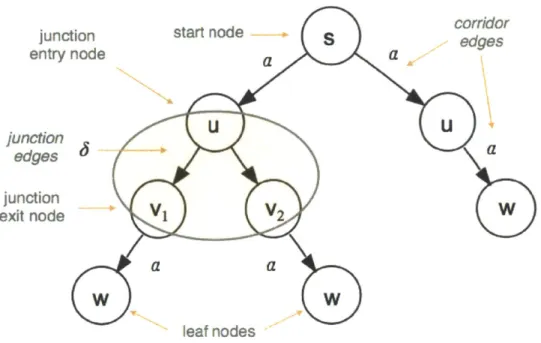
4-1 Minimal subtree that illustrates the mechanics of the optimal pursuit

strategy. Such a subtree would typically be a small part of a large tree

that represents a real-world environment. . . . .

55

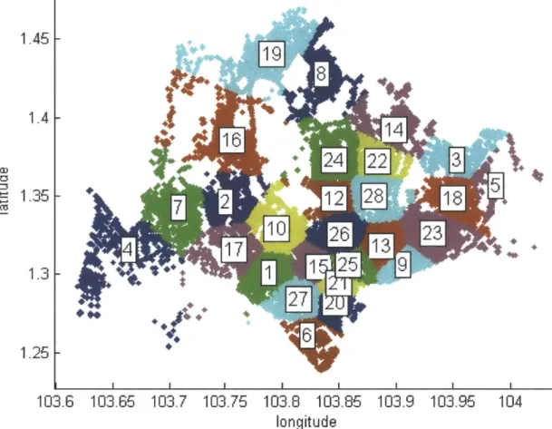
5-1 The 42,000 Singapore nodes used in this study, color-coded according to their k-means clustering. (The computed clusters align well with postal regions in Singapore.) . . . . 62

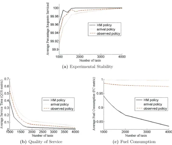
6-1 Simulation Results. Fig. 6-1a shows the percentage of requests serviced for each policy with increasing n. Fig. 6-1b shows the decrease in service time for each policy with increasing n (QOS metric). Fig. 6-1c shows the improvement in fuel consumption for each policy with increasing n (FC metric). . . . . 69

List of Tables

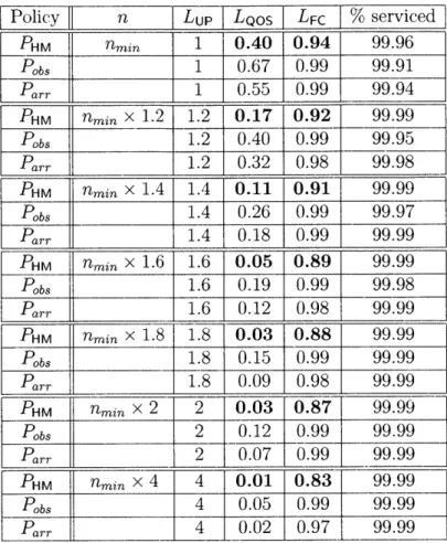
6.1 Simulation Results. A lower metric indicates better performance. The

List of Algorithms

1 Clear Algorithm . . . . 52 2 Practical HM Policy Optimization Algorithm . . . . 68

Chapter 1

Introduction

1.1

Motivations and Goals

Exploration and patrolling are central themes in distributed robotics. The simple

task of deploying a robot to autonomously explore an unknown environment needs

little motivation. With the Curiosity Rover having just celebrated its first birthday

at the time of writing of this thesis, it would not be an overstatement to say that

exploration is one of the most enduring pursuits in robotics.

The goal of exploration is to inspect and obtain a representation of some region

under consideration. The goal of patrolling is to continuously inspect some region

under consideration, while performing certain actions or fulfilling certain problem

con-ditions. These deployment scenarios have obvious direct applications in surveillance,

disaster response, and military operations. But beyond such direct and practical

ap-plications, exploration and patrolling have even deeper fundamental importance in

robotics as they can be used to model an ever wider superset of seemingly unrelated

deployment objectives.

To elaborate, exploration is fundamentally the static acquisition of information

from an environment. In the most general sense, an agent or group of agents

tra-verse an environment and record some kind of sensory data. The objectives of an

exploration task can be different and will inevitably depend on the application in

question. We consider the canonical example, wherein a robot is tasked to traverse

an unknown environment and record a physical map using sensor data. The task is accomplished when data has been gathered from every part of the environment, and the environment is fully mapped. This is the literal interpretation of exploration. But this condition is loose and is malleable to interpretation.

In another example, a robot could be deployed on the battlefield in search of land mines. In this case, the immediate physical environment may or may not be known; the robot may need to clear a specific area, or may need to find a safe path through a certain distance. Any combination of these and other parameters would result in different problems, but all are easily encoded as exploration problems by adjusting the conditions to express the requirements of the problem.

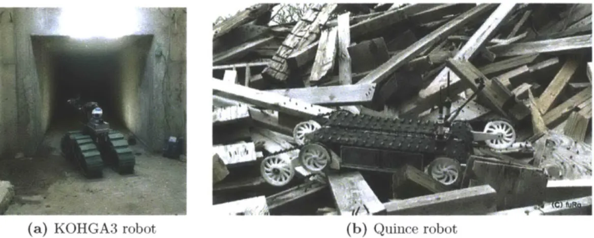
As a final example, we consider a special case of exploration considered in this thesis, called pursuit-evasion. In this scenario, a group of robots are required to sweep an unexplored environment and detect any intruders that are present. Pursuit-evasion is an example of non-recontaminating exploration, whereby an initially unexplored and contaminated region is cleared while ensuring that the cleared region does not become contaminated again. There are interesting real-life applications of pursuit-evasion. Aside from the literal interpretation (pursuing an evader), there are other scenarios that motivate non-recontaminating exploration. For example, in a disaster response scenario following an earthquake, a group of robots is required to locate all survivors in inaccessible areas, while the survivors are possibly moving in the environment. In the aftermath of the Tohoku Earthquake and Tsunami of 2011, the KOHGA3 and Quince search and rescue robots were deployed under these kind of circumstances (Figure 1-1).

Patrolling is an even more general abstraction of such deployment scenarios. Pa-trolling can be interpreted as the dynamic acquisition of data from an environment. In the most general sense, an agent or group of agents traverse an environment and

continuously record some kind of sensory data. It is not hard to see that patrolling is

a generalization of exploration. To motivate this, consider a special case of patrolling where the information being gathered from the environment is constant. If the goal of the task is to continuously acquire this information with time, then a single

ac-it .

(a) KOHGA3 robot (b) Quince robot

Figure 1-1: KOHGA3 and Quince search and rescue robots deployed in the aftermath of the

Tohoku Earthquake and Tsunami of 2011.

quisition is sufficient at all point, as we then have full knowledge of this information thereafter. Thus we can see that this simply reduces to an exploration problem, and exploration in the sense of static data acquisition is a special case of patrolling. If the data source changes with time, acquisition needs to occur continuously, so patrolling can be interpreted as "persistent exploration".

Once again, the goals of a patrolling task depend on the problem being modeled. In the canonical example, a surveillance robot patrols for an intruder in a closed environment. This is the most familiar interpretation of patrolling; in this scenario perhaps the robots are required to patrol regions where intrusion activity is more likely, and avoid safer regions. The task is never "accomplished" as such, since the patrolling is continuous, rather the objective now becomes to provide certain guaran-tees, for example that no intruders enter the patrolled area over a period of time.

To consider another example, a group of autonomous robots may be deployed to cater to an oil spill in the ocean. Following the Deepwater Horizon oil spill of 2010, the Seaswarm oil absorbing robot was deployed for exactly this purpose (Figure 1-2). Such robots may be required to patrol more frequently in regions where there is oil, and avoid clean regions. We may have an estimate of the rate of expansion of surfaced oil based on the hydraulic pressure at the source of the leak. However, we do not know where in the region the oil will surface. The robots patrolling the

(a) Horizon oil spill (b) Seaswarm oil absorbing robot

Figure 1-2: Aerial view of the Deepwater Horizon oil spill, 2010 (left) and the oil absorbing robot deployed in the cleanup efforts (right).

region should cover the entire area at some minimum rate, in order to guarantee that an oil spill will not be greater than a certain radius. Clearly this is a different problem than the previous example, and the objective and criteria for success depend on many different parameters. Nonetheless, these two examples and the previous three exploration examples, can all be encoded as patrolling problems.

Deploying a group of robots, or any type of agent in general, to explore or patrol in dynamic or unknown environments presents us with some fundamental conceptual steps. Regardless of the problem domain or application, we can broadly categorize these as follows. We are required to (a) understand the environment that the agents are being deployed in; (b) encode the task as a set of constraints and guarantees; and (c) derive an effective deployment strategy for the operation of the agents.

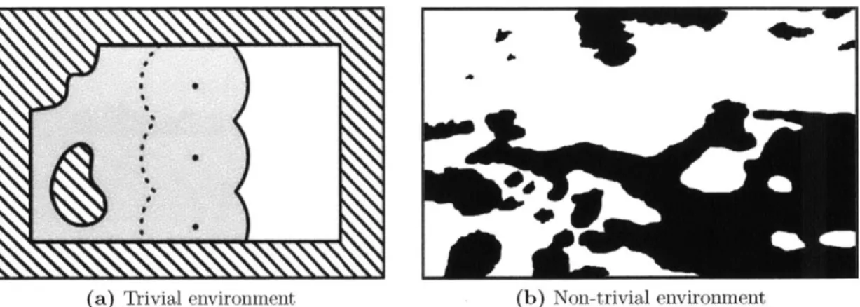
There are notable technical challenges involved in each step. In the first step (a), we need to understand what kind of properties of the environment we are interested in: for example, intuition tells is that width is important; and how they can affect the deployment scenario: the width of the environment may affect the number of agents required to explore it. This is difficult because even in trivial cases it is already unclear how to interpret the simplest geometric parameters (for example in Figure 1-3a it is already unclear how to define the "width" of the environment). In more realistic environments (e.g. Figure 1-3b) our intuition fails and we must be very precise about what kind of metrics we need to obtain and how they relate to the specific scenario

i.9

(a) Trivial environment (b) Non-trivial environment

Figure 1-3: A trivial example environment (left) and a more realistic non-trivial environment

(right). The free region is shown in white and the obstacle region is shown in black.

that is under consideration.

In the second step (b), the difficulty lies in identifying the right level of abstraction for the model. On the one hand, a model that is too simple will not be general enough to express the nuances that fully capture the problem requirements. The problem constraints should be fully captured by the model, and the necessary guarantees should be verifiable from the solution format. On the other hand, if the model is too complicated, it may be difficult to develop a tractable solution and/or to encode the solution as a deployment algorithm. Different levels of abstraction yield different results: some are more general, some more efficient, some more elegant. Which level of abstraction is most suitable depends on the particular requirements of the problem. In the third step (c), the challenge is, put simply, to find a solution that works, and to prove that it works in theory and in practice. The solution can be imperative - an algorithm that directly dictates the deployment of the agents, or it can be passive - a policy that defines a set of rules according to which the agents make decisions as the deployment scenario unfolds. Generally speaking, a sound algorithm or policy should at least guarantee progress and termination. Informally, we understand progress to mean that the algorithm or policy evolves in some progressive manner towards its objective, and we understand termination to mean that the algorithm will eventually complete. Finally, proving that the solution is sound is the primary challenge on the theory front. But equally important is that the solution actually works in a real

application.

This thesis presents a coherent treatment of these steps at the theoretical and practical level. In consideration of the first step (a), we present a novel methodology for understanding an arbitrary continuous environment. We introduce tools for ana-lyzing the environment's underlying topology and geometry. We present an algorithm for obtaining a concise configuration space representation of a physical environment. We derive reasoning about this representation, and show how it can be transformed into a discrete acyclic graph representation of the environment.

In consideration of the second step (b), first we consider a special case of ration called pursuit-evasion. We show how the problem constraints of this explo-ration scenario can be encoded as rules within a discrete environment representation. We establish a mechanism for deploying agents in the environment by casting these rules as a game. We then consider the more general problem of patrolling. We show how a patrolling problem can be set up on a general graph. We encode the prob-lem constraints in a discrete Markov model that faithfully captures all the important properties in problem domain.

In consideration of the final step (c) we present two deployment algorithms. First, we present an exploration algorithm for pursuit-evasion. We show how our environ-ment characterization can be used to derive an algorithm that will guarantee the evaders are detected with the minimum number of pursuers. Second, we present a policy for patrolling on a general graph, and show how this policy is used to solve an important real-life problem in urban transportation. We extend our Markov model to capture the operation of a fleet of service agents (taxis) patrolling the city in re-sponse to incident requests (arriving customers) throughout the day. Our goal is to compute a solution in the form of the required number of taxis in the system and their patrolling policy. We encode the solution as a scalable optimization problem and present a practical patrolling policy.

The thesis presents a coherent treatment of all the steps involved in developing a deployment algorithm for robotic exploration and patrolling: (1) understanding the problem specification, (2) characterizing and representing an arbitrary continuous

environment, (3) transforming the problem into a discrete representation, (4)

devel-oping an effective algorithm to solve the problem, and (5) applying the algorithm to

a real-life application.

1.2

Contributions to Robotics

This thesis makes the following contributions:

" Environment characterization for non-recontaminating exploration.

The first part of this thesis addresses the problem of obtaining a concise

descrip-tion of a physical environment for robotic exploradescrip-tion. We aim to determine the

number of robots required to clear an environment using non-recontaminating

exploration. We introduce the medial axis as a configuration space and derive a

mathematical representation of a continuous environment that captures its

un-derlying topology and geometry. We show that this representation provides a

concise description of arbitrary environments, and that reasoning about points

in this representation is equivalent to reasoning about robots in physical space.

" Deployment strategy for non-recontaminating exploration. We

lever-age our continuous environment representation to derive a lower bound on the

number of required pursuers required to explore the environment using

non-recontaminating exploration. We provide a transformation from this continuous

representation into a symbolic representation. Finally, we present a generalized

pursuit-evasion algorithm. Given an environment we can compute how many

pursuers we need, and generate an optimal pursuit strategy that will guarantee

the evaders are detected with the minimum number of pursuers.

* Markov-Based Model for Urban Mobility Networks. In the second part

of this thesis we present a Markov-based urban transportation model that

cap-tures the operation of a fleet of taxis in response to incident customer arrivals

throughout the city. We leverage data from a fleet of 16,000 taxis in

Singa-pore to create a realistic model of taxi fleet operation in SingaSinga-pore. We show

that a standard undirected clique model is highly restrictive in terms of the kind of transportation network that it can describe. We present an improved model and discuss the steps taken to ensure that the model is realistic while still complying with the Markov framework. We then present a mechanism by which an optimization problem can be set up to handle a sparse network while maintaining a computational complexity that is independent of the degree of precision of the model.

Deployment strategy for patrolling a Markov-based graph model, with application to urban mobility systems. Using the above urban trans-portation model, we show how we can learn and interpret the current default behavior of taxi drivers within our framework, and prove that the current be-havior is sub-optimal with respect to several evaluation criteria. We show how to compute a solution in the form of the required number of vehicles in the sys-ten and their redistribution policy. We then consider the solution with respect to three seemingly different optimization criteria. The first criterion consid-ers the customconsid-ers, whose end goal is to minimize the time spent waiting for a taxi. The second criterion considers the urban planning authority whose goal is to minimize the number of vehicles in the road network. The third criterion considers the cost and environmental implications of fuel consumption. We en-code the solution as a scalable optimization problem and present a practical redistribution policy.

* Experiments. We evaluate our policy by comparing it against the actual observed redistribution of taxi drivers in Singapore. We present experimental results via implementation in large-scale traffic simulations and consider the extent to which optimization at different levels of abstraction can work together as part of a complete urban mobility system. We show that our proposed policy is stable and improves substantially upon the default unmanaged redistribution of taxi drivers in Singapore with respect to the three optimization criteria.

1.3

Relation to Previous Work

An important aim of our work is to bridge the different levels of abstraction that work

to date has been grounded in. This section elaborates on this claim, and highlights

the motivations for improvement over the existing state of the art. Chapter 2 provides

a comprehensive survey of related work.

Environment characterization for pursuit-evasion has been considered for

polygo-nal spaces. We highlight that these studies considered robots equipped with infinite

range visibility sensors deployed in polygonal spaces. Consequently the scope of

en-vironment characterization was limited. By contrast we consider limited visibility

sensors, and we do not require the environment to be polygonal.

The medial axis has previously been studied in the context of robotic navigation.

In this work, we use the medial axis to capture the underlying topological and

ge-ometric properties of our environment, and use it to transform the problem into a

graph formulation. In our work, we consider the medial axis in a completely novel way

- by treating it as a configuration space to derive a robust representation of a

con-tinuous environment that captures its underlying properties. We then use the medial

axis we then leverage existing exploration models to build a concise representation of

arbitrary environments in continuous two-dimensional space.

Visibility-based pursuit-evasion has been considered for continuous two-dimensional

spaces. Generally speaking, visibility-based algorithms do the correct thing locally,

but do not rely on, or make any guarantees for, a global description of an environment.

As such, they may not be guaranteed to terminate.

Pursuit-evasion on graphs that are representations of some environment date back

more than four decades. Although discrete graph-based models offer termination and

correctness guarantees, they assume the world is suitably characterized and make

no reference to the underlying physical geometry of the environment that is being

represented.

In our work, we make use of the medial axis to establish a transformation from

a continuous representation of an environment into the discrete domain. First, this

allows us to calculate bounds on the number of robots required to clear an environ-ment, and to provide termination guarantees for existing pursuit-evasion algorithms. Second, this establishes an application platform for existing graph-based algorithms making them applicable to continuous environment descriptions.

More generally, we establish techniques which can in principle be used to trans-form a low-level continuous representation into a high-level graph-based discrete rep-resentation, and thus offer a mechanism for transforming any low-level exploration or patrolling problem into high-level problem.

Many different application scenarios of the exploration and patrolling model have been studied, as motivated by the examples in the preceding discussion and in Figures 1-1 and 1-2. As an end point for our work we consider an application of some practical significance - urban mobility has been an active area of research since the turn of the century. In the US, the annual congestion cost is projected to grow to $133 billion by 2015 [22]. Not surprisingly, social and municipal trends are changing in favor of a modernized system of public transportation, and the recent volume of research in the subject reflects this.

Dynamic Traffic Assignment problems generally aim to optimized traffic flow while accounting for congestion effects. DTA models commonly differ widely in the rep-resentation of the supply and demand processes. Mobility-on-Demand (MOD) is a newer paradigm for handling traffic congestion. The Pickup and Delivery prob-lem (PDP) is a paradigm for handling traffic congestion whereby passengers arriving into a network are transported to a delivery site by vehicles. Load balancing in the Mobility-on-Demand systems is a similar a problem. As well as system-level traffic flow considerations, socially motivated objectives have also been considered, where the collective optimization criteria of the entire system are incentivized in favor of individual optima.

DTA and PDP problems are characterized by inherent mathematical intractabil-ity and challenging complexities. One practical consequence of this is that research has favored the development of heuristic solutions that emphasize effectiveness, ro-bustness, and deployment efficiency over claims of uniqueness or global optimality

that may not be essential or particularly meaningful in the practical applications. As

such, solutions tend to be less general, and are useful within narrow margins of the

problem context.

Our work extends to encompass a broad scope of optimization criteria. We

con-sider the interplay between global optimization criteria typical of related studies of

DTA and MOD systems, as well as social optimization criteria as motivated by recent

studies of congestion-aware traffic systems.

We believe that urban mobility is an exciting application scenario for robotics

al-gorithms, in particular for the following reason. Infrastructure and technology

devel-opments are resulting in MOD systems becoming "smart" to varying degrees. Vehicles

can now drive themselves and human drivers often rely on automated navigation

sys-tems. The lines between what is a manned system and what is an autonomous system

are becoming blurred. Developments in distributed robotics are becoming ever more

pertinent to vehicle operation, navigation systems and traffic networks. The

applica-tion of our algorithms tradiapplica-tionally developed for autonomous robots to human taxi

drivers offers us new insights into transportation systems and sets precedent for the

urban mobility systems of the future.

1.4

Thesis Organization

This thesis is organized into eight chapters. Chapter 2 provides a comprehensive

survey of related work. Chapter 3 presents a mechanism for obtaining a concise

representation of a physical environment for robotic exploration. Chapter 4 presents

an optimal deployment algorithm for a group of robots engaged in distributed

non-recontaminating exploration. Chapter 5 presents a Markov-based urban mobility

model and a mechanism by which a group of robots can patrol the graph to service

persistent requests. Chapter 6 presents a practical deployment policy for patrolling

the urban mobility model and shows how our algorithm offers several improvements

over current ground truth behavior. We conclude the thesis in Chapter 7, reflect on

the contributions of the work and consider lessons learned for future work in this area.

Chapter 2

Related Work

This thesis builds on ground-breaking prior research in robotic algorithms for explo-ration, pursuit-evasion, and task allocation. The research also builds on prior research on modeling and lower bounds for decentralized algorithms. In this chapter we detail some of the key results.

2.1

Exploration, Pursuit-Evasion and Patrolling

Visibility-based pursuit-evasion in continuous two-dimensional space was first intro-duced in [43]. Frontier-based exploration was introintro-duced in [49] and extended to multiple robots in [50]. In [10] the authors consider limited visibility frontier-based pursuit-evasion in non-polygonal environments, making use of the fact that not al-lowing recontamination means we do not need to store a map of the environment; here a distributed algorithm is presented which works by locally updating the frontier formed by the sensor footprints of the robots. Another distributed model was more recently considered in [6]. Limited visibility was also considered in [41] which presents an algorithm for clearing an unknown environment without localization. In [13] the problem was considered for a single searcher in a known environment.

Environment characterization for pursuit-evasion has been considered for polygo-nal spaces. In [15],[17] pursuit-evasion in connected polygopolygo-nal spaces is investigated, and tight bounds derived on the number of pursuers necessary based on the number of

polygon edges and holes. In [29] basic environment characterization is established, by

means of a general decomposition concept based on a finite complex of conservative

cells. In [48] similar ideas were explored, and several metrics proposed for primitive

characterization of polygonal spaces.

The medial axis has previously been studied in the context of robotic navigation.

For example, in [16],[20],[47] the medial axis was used as a heuristic for probabilistic

roadmap planning. One of the key features that makes the medial axis attractive for

such applications is that it captures the connectivity of the free space.

Pursuit-evasion on graphs that are representations of some environment goes back

as early as [33],[35]. Randomized pursuit strategies on a graph are considered in [1].

Roadmap-based pursuit-evasion is considered in [24] and [39] where the pursuer and

evader share a map and act according to different rules. In [39] a graph-based

repre-sentation of the environment is used to derive heuristic policies in various scenarios.

More recently, [27] presents a graph-based approach to the pursuit-evasion problem

whereby robots use blocking or sweeping actions to detect all intruders in the

envi-ronment. In [25] and [26] the more general graph variant of the problem was reduced

to a tree by blocking edges.

Many other approaches and starting assumptions have been explored.

Proba-bilistic evader detection, where multiple searchers are tasked with efficiently locating

evaders is studied in [21], while [19] presents a greedy probabilistic policy for multiple

pursuers. Roadmap-based pursuit-evasion, where the pursuer and evader share a map

and act according to different rules is studied in [24] and [39]. Randomized pursuit

strategies under different conditions are investigated in [23]. An adaptive planning

strategy for pursuit-evasion in unknown environments is presented in [2].

2.2

Applications to Urban Mobility

The Dynamic Traffic Assignment problem (DTA) dates back as early as [31] and

[12]. Generally speaking, the objective of DTA problems is to optimize traffic flow

while accounting for congestion effects. A thorough survey can be found in [38]. For

example, the problem is grounded in continuous time control theory in [12], while [11] presents a variational inequality formulation. A mathematical programming approach in used in [31], [51]. Another recent work [51] models the problem as a linear program, and a simulation-based approach in [3] presents an offline model for estimation of supply and demand.

Mobility-on-Demand (MOD) is an emerging paradigm for handling traffic conges-tion. In MOD systems, the goal is to provide users with on-demand rental facilities of convenient and efficient modes of transportation [32]. Load balancing in MOD systems is similar to the Pickup and Delivery problem (PDP), whereby passengers arriving into a network are transported to a delivery site by vehicles. For a review of the state of the art see [4], [34] and the references therein. Autonomous load re-balancing in MOD systems has recently been studied in [36] and [37], where a fluid model was used to represent supply and demand.

As well as system-level traffic flow optimizations, socially motivated criteria have also been considered. Recent work on traffic planning explored optimizing a drivers's route subject to congestion [30]. Social optimum planning models for computing vehicle paths are presented in [40, 46].

Chapter 3

Environment Characterization for

Non-Recontaminating Exploration

This chapter addresses the problem of obtaining a concise description of a physical

environment for robotic exploration. We aim to determine the number of robots

re-quired to clear an environment using non-recontaminating exploration. We introduce

the medial axis as a configuration space and derive a mathematical representation of a

continuous environment that captures its underlying topology and geometry. We show

that this representation provides a concise description of arbitrary environments, and

that reasoning about points in this representation is equivalent to reasoning about

robots in physical space. Finally, we leverage this representation to derive a lower

bound on the number of required pursuers.

This chapter of the thesis is organized as follows. In Section 3.1 we provide a

formal model for non-recontaminating exploration and state the problem that we are

addressing. In Section 3.2 we introduce the medial axis as a configuration space and

show that reasoning about points in this space is equivalent to reasoning about robots

in the physical world. We formalize the notion of width, corridors and junctions and

derive bounds on the number of robots required to traverse a junction.

3.1

Problem Formulation

We now present a formal model of the problem we are addressing. Our model builds on the notation and terminology introduced in [10]. We have a team of n exploration robots deployed in the Euclidean plane R2. Each robot is equipped with a holonomic (uniform in all orientations) sensor that records a line of sight perception of the environment within a maximum sensing radius r. We assume that two robots can reliably communicate if they are within line of sight of each other and if the distance between their positions is less than or equal to 2r.

The position of a robot is constrained to be within some

free

region

Q,

which is a closed compact subset of R2. The obstacle region B makes up the rest of the world, and is defined as the complement of

Q.

In this work we require both

Q

and B to be connected spaces, which means there are no holes in the environment. We define the obstacle boundary BB as the oriented boundary of the obstacle region (which by definition is the oriented boundary of the free region).

We assume a continuous time model, i.e. time t E R>o. Let Ht be the holonomic

sensor

footprint

of robot i at time t, which is defined as the subset of

Q

that is within direct line of sight of robot i and within distance r of robot i. Formally, if p E R2 is the position of robot i at time t, then Hti

{x

c

Q

I

d(p, x) < r A Vy E [px] , y E

Q}

where d(x, y) is the Euclidean distance between x and y (see Fig. 3-1a). Let

H

be the union of the sensor footprints of all robots at some time t, given by Hit -

Un

₀ Ht. This

corresponds to the region being sensed by the robots at time t. We define the inspected

region It C

Q

as the union at time t of all previously recorded sensor footprints,

given by It = {p E R

2

I

Eto E [0, t] such that p E Hto}. The contaminated region (or

unexplored region) Ut is defined as the free space that has not been inspected by time

t, given by Ut =

Q

\

It (see Fig. 3-1b). Note that at time t = 0 the contaminated

region is given by

Q

\

Ho. We define the cleared region Ct g

It

as the inspected region that is not currently being sensed, given by Ct = It \ Ht. We say that recontamination occurs at time t if the cleared region Ct comes in contact with the contaminated region

Q1 H

(a) Sensor Footprint (b) Inspected region (c) Boundaries

Figure 3-1: Fig. 3-la shows a robot located at some position p within the free region Q. The sensor footprint H and its oriented boundary OH are shown on the right. Fig. 3-1b shows the inspected region It and the contaminated region Ut at some time t. Fig. 3-1c shows the inspected region boundary 01, the inspected obstacle boundary DIB and the frontier Y.

non-empty, i.e.

cl(Ct)

n cl(Ut)

#

0).

When time is clear from context, we understand I and U to mean the current inspected region and the current contaminated region, respectively. We define the

inspected region boundary aI as the oriented boundary of the inspected region I. We

define the inspected obstacle boundary 0 1_B

as the intersection of the inspected region boundary and the obstacle boundary, given by aIB = aI

n &B.

We define the frontier F as the free (non-obstacle) boundary of the inspected region, given by F =i \ 81

B

(see Fig. 3-1c). Observe that by definition the frontier F separates the free region

Q

into the inspected region I and the contaminated region U. Observe also that the frontier need not be connected, and is in general the union of one or more disjoint maximally connected arcs. We understand the frontier of a group of robots F' C F

to mean a single maximally connected arc of the total frontier formed by the exterior boundary of the sensor footprints of that group of robots.

The goal of exploration algorithms is to inspect the entire free region. For non-recontaminating exploration the goal is to inspect the entire fee region without ad-mitting recontamination. In both cases we say that an environment has been suc-cessfully explored if It =

Q

at some time t. In this thesis we deal specifically with non-recontaminating exploration and present an algorithm that is guaranteed to ex-plore a space without admitting recontamination.

An algorithm for exploration relies on robots to "expand" the frontier boundary until the entire free region becomes inspected. However, in a non-recontaminating exploration algorithm the goal is not only to expand, but also to "guard" the

fron-tier, ensuring that the inspected region does not become contaminated again. This difference makes non-recontaminating exploration more restrictive than conventional exploration. For example, observe that regardless of the size of the sensing radius of the robots (as long as r > 0), or the properties of the world (as long as

Q

is a connected space), a single robot can always explore the world. However, in non-recontaminating exploration this is not true in general. Informally speaking, if the "width" of the corridors in the free region is larger than the sensing radius of a robot, then it should appear obvious that a single robot cannot simultaneously expand and guard the frontier to inspect the entire free region.

Consider the simple rectangular free region

Q

shown in Fig. 3-1b. We can reason that if the width of

Q

is less than the sum of the sensor diameters of the n robots, then the environment can be explored without admitting recontamination. However, even in this simple example it is not completely clear what is meant by width. Notice that if we consider width to be the distance from the left to the right border then this reasoning fails -- in this case width would specifically mean the smaller of the two dimensions. So it is already non-trivial how to characterize a very simple environment, and things become much more complicated in non-rectangular environments.

In this thesis we study the relationship between an environment

Q,

the sensor radius r, and the number of robots n required for non-recontaminating exploration of

Q.

Intuition tells us that corridor width and junctions are important features. We formalize the notion of corridors and junctions and present a general method for computing a configuration space representation of the environment that captures this intuition. We show that this representation provides a concise description of arbitrary environments.

A canonical example of non-recontaminating exploration is pursuit-evasion. In this scenario there is a group of robot pursuers and a group of robot evaders deployed in the free region

Q.

The evaders are assumed to be arbitrarily small and fast. The goal of the pursuers is to catch the evaders (by detecting their presence within the sensor footprint), and the goal of the evaders is to avoid getting caught. Whenever part of the frontier is not being guarded by the pursuers, the evaders can move

undetected from the contaminated region to the previously inspected region, thereby

recontaminating it.

3.2

Environment Analysis

In this section we present the medial axis as a configuration space and show that

reasoning about points in this configuration space is equivalent to reasoning about

robots in physical space. First, we establish the necessary geometric framework,

accompanied by a series of definitions and claims. Second, we introduce an exploration

model in this configuration space and justify that it allows us to reason about the

physical movement of the robots in the environment.

3.2.1

Environment Geometry

The distance transform is a mapping D :

R2 -+

R where D(x)

= minyCB

{d(x, y)}

and d(x, y) is the Euclidean distance between x and y (extending definition in [8] to

the continuous domain) (see Fig. 3-2b). Observe that by definition if x (

Q

then

D(x)

=

0. The distance transform of a point x

_c

Q

_{captures the notion of "undirected}

width" of a region around a point x in free space, that is we get a measure of how

wide or narrow a region is without being explicit about orientation.

The medial axis or skeleton S of a free space is defined as the locus of the centers

of all maximal inscribed circles in the free space [7] (see Fig. 3-2c). Equivalently, the

skeleton can be defined as the locus of quench points of a fire that has been set to

a grass meadow at all points along its boundary [5], [42]. The skeleton captures the

topology of the free space, and aids us in determining which parts of an environment

should be considered "corridors" and which parts should be considered "junctions"

of multiple corridors.

The degree of a point x E S is given by the function 0 : S

-+

N>o which maps

every point on the skeleton to a natural number k. Specifically, we define a point

x

c

S to have degree 0(x)

=

_{k if there exists an a E R>o such that Ve E (0, a] a circle}

(a) Environment image (b) Distance transform (c) Skeleton (d) Relief map

Figure 3-2: The environment is represented by a binary image in Fig. 3-2a. Fig. 3-2b shows the distance transform D of the environment. Fig. 3-2c shows the skeleton S. Fig. 3-2d shows the relief map quantization. The relief contours indicate multiples of the sensing radius r.

Borrowing notation from [9], we use the degree of a point x E S to distinguish

between three types of points on the skeleton: corridor points, end points and junction points. Specifically, for a point x c S, we say x is an end point if 0(x) = 1, x is a

corridor point if 0(x) = 2, and x is a

Junction

point if 0(x) > 2 (see Fig. 3-3a). We

refer to a continuous are of corridor points on the skeleton simply as a corridor. An alternative definition for 0(-) can be stated as follows. For a point x E S let C be the maximal inscribed circle centered at x, and let G be the intersection of this circle with the obstacle boundary, given by G = C

n

DB. (Observe that by definition C has radius D(x) y- 0, and since C is maximal, G is non-empty.) Then 0(x) is defined as the number of maximally connected arcs in G. This definition for for 0(-)

is equivalent to the previous one [7], [14], [28].

Let G1, G2,... , Go(x) be the set of maximally connected arcs of G. Note that in

most cases these arcs are in fact just single points, which corresponds to the intuitive notion of the circle being tangent to the boundary at these points. A cursory glance reveals that this is the case for most corridor points and junction points. For end points that lie on the obstacle boundary, the tangent point coincides with the end point itself. However, the generality is necessary in a few special cases, such as end points of regions that taper off in a sector. In these cases the maximal inscribed circle C will be tangent to the obstacle boundary at a continuous are segment of points. In order to simplify the discussion we define the tangent points Ti(x), 72(x), .. , TO(x)

of a point x E S as the midpoints of the tangent arcs G1, G2, .. ., Go(x) (see Fig. 3-3b).

We define a boundary wall as a maximally connected are segment of the obstacle boundary DB that does not contain a tangent point of any end point. Formally

C B OB r2 Q _Q 6(x) = 1 (e) r* n,(e) 9(z) = 3 .)() 4 e, 71(e;-) ... U() ---(z)= 2

(a) Skeleton points (b) Dead end tangent point (c) Junction tangent points

Figure 3-3: _{Fig. 3-3a shows the three types of points on the skeleton: end points, corridor points,}

and junction points. A corridor is a continuous are of corridor points. Fig. 3-3b shows three points on the skeleton e, e', j _{and their respective tangent points. For end point e the tangent point} Ti (e) is

the midpoint of the tangent arc segment shown (dotted outline). For end point e' the tangent point Ti(e') _{coincides with the end point itself. For junction point j there are 6(j) = 3 tangent points}

Ti, T2, T3. Fig. 3-3c shows a junction point

j

of degree 0(j) = 3. All 3 tangent points Ti, T2, T3 are

located on distinct boundary walls.

OBo

c

_{OB is a boundary wall if it is a maximally connected are segment such that}

Ve E S

I

0(e)

= 1, r(e) 0 BBo_.

Lemma 1. For a junction point

j

E S, the 0(j) tangent points of

j

are located on 0(j) distinct boundary walls.

Proof. A circle C of radius D(j) centered at a junction point

j

will be tangent to

the obstacle boundary at the 0(j) tangent points of

j.

Each pair of adjacent tangent points ri, Ti.1 _{E C (in the sense of counter-clockwise orientation along C) will be on}

opposite sides of one corridor. Consider the obstacle boundary arc segment [Ti Ti+1]

(in the sense of counter-clockwise orientation along OB). If e is the end point of the corridor that straddles the interior of [Ti ri+1], then r(e) will lie on [ri Ti+1]. Thus the boundary wall containing ri is disjoint from the boundary wall containing Ti.1 since neither contains T(e). _{Since this applies for each pair of adjacent tangent points, we}

conclude that all 0(j) tangent points Ti, T₂,. . ., TO6 ) will be located on 0(j) distinct

boundary walls (see Fig. 3-3c). 0 El

3.2.2

Exploration Model

We now show how we can use the preceding definitions and geometric claims to form a model for frontier-based exploration and establish an equivalence between the the medial axis configuration space and the physical environment.

We claim that reasoning about a single point moving along the skeleton allows us to reason about a group of robots that form a frontier with their end to end sensor footprints moving through physical space. We call this point the swarm locus. By definition a corridor point x

c

S has exactly two tangent points. For a swarm locus stationed at x we call these two points the frontier anchor points. The frontier of a group of robots is represented by a corresponding frontier formed by two line segments joining the swarm locus to its anchor points. A group of robots engaged in non-recontaminating exploration will form a frontier arc subtended between two obstacle boundary walls in physical space; the frontier arc separates the inspected region on one side from the contaminated region on the other side. Our abstraction allows us to reason in similar terms: a swarm locus stationed at a point x on the corridor of the skeleton will similarly form a frontier arc consisting of two line segments subtended between two obstacle boundary walls; the frontier arc transposed onto

Q

likewise separates the inspected region from the contaminated region (see Fig. 3-4a). We understand the frontier of a swarm locus to mean the frontier F' C F of a group of robots represented by a swarm locus stationed at a point x E S.

Note that we are making a simplifying abstraction in representing the frontier F' C F of a group of no robots by two end to end line segments subtended between two obstacle boundary walls. Observe that as n grows, the abstraction becomes more accurate as the periodic protrusion of the frontier due to the curvature of sensor footprints becomes finer-grained and less prominent with respect to its length. In general, this abstraction is justified as we are usually interested in characterizing environments where n

>

0.

For the purposes of introducing the exploration model we assume that the swarm locus always begins at an end point. (Note that this assumption only serves to simplify the discussion, and can be removed easily by introducing several special cases.) From the definition of the degree of a point on the skeleton, a maximal inscribed circle C centered at an end point e E S will be tangent to the obstacle boundary at a single point T(e). Thus both anchor points are the same point r(e) and the frontier F' C F of a swarm locus stationed at e is formed by two identical line segments [e T(e)]. In

I Uk 1

k Uk

F S

F' S \

e

x

swarm locus"

~

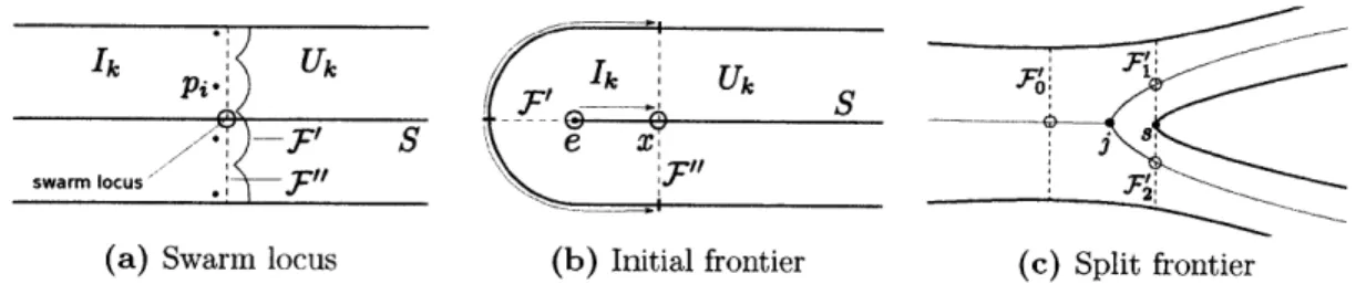
,F".~

(a) Swarm locus (b) Initial frontier (c) Split frontier

Figure 3-4: Fig. 3-4a shows a group of robots at positions pi forming a frontier F' with the exterior boundary of their sensor footprints. Superimposed is the corresponding swarm locus stationed at a point x E S forming a frontier F" with two line segments subtended between two obstacle boundary walls. Fig. 3-4b shows the initial frontier F' of a swarm locus stationed at an end point e, separating the environment into Io = 0 and Uo = Q. As the swarm locus moves along the skeleton to reach a point x E S, it forms a frontier F". The swarm locus has swept across the environment and cleared the region to the left of F". Fig. 3-4c shows the configuration of a split frontier. A swarm locus is traversing a junction point j with 6(j) = _{3. The ingoing frontier F splits, producing 1 split point}

s and 2 outgoing frontiers F{, F{.

this configuration, F' separates the environment

Q

into the inspected region

1

_o

₌

₀

and the contaminated region Uo

=

Q,

corresponding to the fact that the swarm locus

has not yet explored any of the environment. As the swarm locus starts moving along

the skeleton, the anchor points will move along 9B on either side of the corridor

and the frontier will "sweep" across the environment. The frontier now separates

Q

into two disjoint nonempty regions. The inspected region begins growing, while the

contaminated region begins shrinking, corresponding to the fact that the robots have

begun clearing the environment (see Fig. 3-4b).

Moving Through Corridors

We define the relief map R : R2 --+ N as the quantization of the distance transform

using the sensing radius r, given by R(x)

=

[D(x)/r] (see Fig. 3-2d). The relief map

uses the distance transform to similarly capture the notion of width, expressing the

same information in terms of the number of robots required at a point x to reach the

closest point on the obstacle boundary.

Lemma 2. A group of no robots represented by a swarm locus that reaches a

corridor

point x G S prevents recontamination if and only if no > R(x).

Proof. In order to prevent recontamination, the group of robots must subtend a

frontier between two obstacle boundary walls in physical space. By definition, the