Density perturbations in hybrid inflation

Density Perturbations in Hybrid Inflation

by

Nguyen Thanh Son

Submitted to the Department of Physics

in partial fulfillment of the requirements for the degree of

Master of Science

at the

MASSACHUSETTS INSTITUTE OF TECHNOLOGY

September 2009

MASSACHU3ETTS INSTITUTE

OF TECHNOLOGY

AUG

R

i

2012

,.LIBRARIES

@

Massachusetts Institute of Technology 2009. All rights reserved.

Author ...

Department of Physics

July 28, 2009

Certified by...

Alan H. Guth

Victor F. Weisskopf Professor of Physics

Thesis Supervisor

Accepted by ...

... . .... .. .... ...,. .

Tho

s J. Greytak

Associate Department Head for Education

Density Perturbations in Hybrid Inflation

by

Nguyen Thanh Son

Submitted to the Department of Physics on July 28, 2009, in partial fulfillment of the

requirements for the degree of Master of Science

Abstract

Inflation is a substantial modification to the big bang theory, and supernatural infla-tion is a hybrid inflainfla-tion motivated from supersymmetry. In this thesis we carry out a one dimensional numerical simulation to verify the untested analytic approximation of Radall et al. The results show a good agreement for a wide range of parameters. We also propose a new method for calculating density perturbations in hybrid inflation, which shows an excellent agreement with the simulation in one dimension.

Thesis Supervisor: Alan H. Guth

Acknowledgments

I first wish to thank my advisor Alan Guth for his invaluable help on both physics and

non-physics matters. It has always been a pleasure and honor to work with him. I wish to thank Hong Liu and Xingang Chen for their knowledge and advices. I wish to thank my collaborator Carlos Santana for his patience and enthusiasm. I am honored to be a fellow of the Vietnam Education Foundation. And last but not least, I wish to thank my parents Nguyen Trung Thuan and Doan Thi Phong for their endless support and encouragement, my companion Dang Thi La Thu for her understanding and sharing, my undergraduate research advisor Nguyen Quoc Khanh for leading me through the very first steps of scientific research, and all friends and teachers that I

Contents

1 Hybrid Inflation

1.1 Classical evolution . . . .. . ... .. . . . . .. . . . . .

1.2 Expansion in M odes . . . .

2 Time Delay Method

2.1 Time Delay Definition ... ...

2.2 Proof That Time Delay Is Fixed ...

2.3 Randall-Soljacic-Guth Approximation ... 3 Numerical simulation

3.1 Field evolution ...

3.2 The ending time . . . .

3.3 Monte Carlo Simulation . . . .

3.4 The Direct Integration Method

3.5 Variation of the time delay field

3.6 Conclusions . . . . 7 8 10 14 15 17 17 20 . . . . 20 . . . . 2 2 . . . . 2 3 . . . . 26 . . . . 3 1 . . . . 34

List of Figures

1-1 Mode function for k/H =1/256, 1/16, 1, 16, 256 . . . . 12

2-1 RSG approximation for different sets of physical parameters. . . . . . 19

3-1 Compare the RSG approximation with the Monte Carlo simulation.

The rescaling parameters are krescaled = 2.2k, ATrescaled = 0.63AT. . . . 23 3-2 Compare the direct integration method with the Monte Carlo

simula-tion. The parameters are po = 18 and pV, = 1/22 . . . . . 30 3-3 The mean ending time. . . . . 32

List of Tables

3.1 Change the physical parameters yo and [p with fixed product p1y0 . 24

3.2 Compare our simulation results with Burgess' for po = 18 and pbk = 1/22. 25

Chapter 1

Hybrid Inflation

Inflation is the epoch when the energy density of the universe is dominated by the potential energy of a scalar field. During this epoch, the scalar field is either trapped in a false vacuum or slowly rolling down a hill, the energy density of the universe is approximately constant, and the scale factor is exponentially growing with time.

Inflation was first introduced to solve the problem of magnetic monopoles pre-dicted by Grand Unified Theories[3]. By adding an epoch of exponential expansion, any unwanted relic produced before inflation will be diluted away. It was shown later that inflation also provides an explanation for the flatness and the horizon problems of the Standard Model of Cosmology. Recent measurements confirmed the prediction of inflation for scale-invariant density perturbations and a flat universe.

However, inflation does face the naturalness problem: most inflation potentials have small parameters, either to have the correct order of magnitude for the density perturbations or to have enough e-foldings. One way to get over this difficulty is to construct an inflation potential with small parameters that already existed in particle physics so that we do not need to introduce new ones. This is the motivation for Supernatural Inflation[7], a hybrid inflation model with a potential motivated from supersymmetry. As with other hybrid inflation models, supernatural inflation does not have a classical solution for the evolution of the scalar field, to which quantum fluctuations can be treated as small perturbations. The authors of Supernatural

We will validate the approximation by comparing with a Monte Carlo simulation. Kristin Burgess in her Ph.D. thesis [2] has reached the conclusion that the analytic approximation and the simulation are in good agreement provided that we rescale both the amplitude and the wave number of the analytic calculation for density perturbation by two factors of order 1. The aim of this thesis is to go one step further

by investigating the dependence of these factors on the model parameters.

1.1

Classical evolution

We will consider a scalar field in a fixed background de-Sitter space, with the scale factor

a(t) = e Ht

where H is the Hubble constant during inflation. The scalar field <0 is described by the Lagrangian density

Lp = eHt 2 _ -2HtV 2 2t (1.2)

In a typical single field inflation the mass term would be time-independent. In a hybrid inflation, however, the mass term is controlled by the second scalar field which acts as the switch to end inflation. We will consider the mass term of the form:

m2(t) = -m - (I(1.3)

We will set r = 4 in the simulation. The second scalar field is described by another Lagrangian density but with fixed mass

LO = eHt [ 2 _ e-2Ht(VV) 2 - 2m

j2

(1.4)

Note that the Lagrangian densities are defined up to additive constants. These con-stants will be defined to have sufficient values for negligible variation of H during inflation.

The equations of motion are

$ + 3H - e-2_{H V}2 _{=-T (1.5)}

b+ H - e- 2HtV2 -2 (1.6)

Using the slow-roll approximation for the 0 field, we get the evolution as:

0(t) = oce-(m /)(.7

The integration constant was chosen so that b = 'c and m 2(t) = 0 at t = 0. The

mass term for

#

becomes

2 2 [1_-rp rN] 18

m=- iM₀ [ -1-8)

where we have defined

N Ht

P m0/H (1.9)

With the mass term (1.8), the scalar field

#

has two separate stages of evolution

" Oscillation N < 0, m2 > 0: The

#

field is trapped at its local minimum. Classically, there will be no fluctuation, and

#

will stay at the same value even when the potential flipped. Quantum mechanically,

#

will oscillate around the minimum, and those quantum fluctuations will provide the initial deviations for rolling down in the tachyon stage.

* Tachyon N > 0, m2 < 0: potential flipped,

#

has negative effective squared mass and will roll down the potential hill until reaching a new minimum.

In our toy model, which is constructed as a free field theory, the

#

field will roll down forever. For ending inflation, instead of reaching a true minimum, the

#

field will

1.2

Expansion in Modes

We will approximate space by a lattice so that the problem can be solved numerically To make the calculations as efficient as possible, we work in one space dimension. Although we are really interested in three dimensions, the one-dimensional model will allow us to test the analytic approximation that will be described in Section 2.3. Assume, therefore, that the space consists of a box of fixed coordinate length b, with periodic boundary conditions with

Q

independent points. In the computer program, the number of points

Q

will be chosen as a power of 2 (Q = 217) so that we can use

the Fast Fourier Transform algorithm to speed up the calculation.

X = --b (1.10)

Q

where 1 = 0, 1, ..., (Q - 1). And the wave number is

27r

k = b "(1.11)

b

with n running from -Q/2 to (Q/2) -1. Because of the periodic boundary condition, only one value of k on the boundary is needed.

The mode expansion of the scalar field is

1 1 [27r- 1/2 (Q/2)-l k i-U

#(x, t) =

[2j

Y

[c(k)eikxu(k, t) + dt(k)e-iku*(k, t)]

/ b _-/n=-Q/2

eikx [c(k)u(k, t) + dt(-k)u*(-k, t)] (1.12)

n=-Q/2

where c(k) and dt(k) are creation and annihilation operators. The canonical commu-tation relation of the scalar field is

where

(1.14)

wX(x)

=

--M<b(X)

Using the normalization convention of u(k, t) as in [4] and [2], we can get the commutation relations for the creation and annihilation operators as

[c(k)ct(k')] = [d(k)d t(k')] [(k), dt(k')] = [c(k)c(k')] = t6k,k' = 0 (1.15) (1.16)

Substituting the mode expansion back into the equation of motion, we get the equa-tion for the modes

i + Hit + e-2_Htk2_{u =}

-mo(t)u (1.17)

Define new function and variable as

k

a- _ H u(k, t) (1.18) (1.19) - R(k, t)eo(kt) 2kH

then the equation of motion becomes

ft = -e + R[P2(1 - e-N) k-2 -2N] + S= k2 -2N R3 (1.20) (1.21) keN

At early time, the k term in equation (1.17) dominates over the mo(t) term and the solution will be [4]

u(k, t) = 2 e~-N/2Z(Z)

where

(1.22)

Z = - e-N

4 n5 ,(4 10 3 10 10 2 10 10* 10-10-2 -10 -5 0 Ht 5 10

Figure 1-1: Mode function for k/H =1/256, 1/16, 1, 16, 256

k/H=1/256

---- k/H=1/16

k/H=1

---- k/H=16 k/H=256

and Z(z) satisfies

d2_{Z dZ +}

z2 +Z z

+

-Z2- =0 (1.24)

At early time, the mode functions have the form

1

-u(k, t) ~l eikeN (1.25) 2Hk or in term of R and 0 R - 1 (1.26) 0 k

Ie--N(.7

These equations will be used as the initial conditions for the differential equations (1.20) and (1.21). For numerical calculation, given the values of R(k, t) and R(k, t), we can always use the Runge Kutta method to evaluate the values of R(k, t + dt) and

R(k, t + dt). With the step size dt = 5 x 10-4 in units with H = 1, the error in AR/R

is less than 10-' for the entire rage of t. Some results from these integrations are shown in Fig. 1-1. We can see that all the mode functions increase exponentially at the same rate at late time, which is consistent with the asymptotic form of the mode

equations when N -- oo

R -b + R[p1 e (1.28)

Chapter 2

Time Delay Method

Time delay is a method of calculating the primordial density perturbation[5],[6],[8]. At the end of inflation, the inflation field rolls down a hill in its potential energy diagram toward its true vacuum value. Because of the quantum fluctuations, some regions may reach the end of inflation earlier than others, and therefore have less inflation.

This method has the advantage of being simple and intuitive, but it also has some limitations:

" Valid only if H ~const during inflation.

" Valid only for single field inflation. However, we will make an attempt to use it

for hybrid inflation.

" Requires an assumption of instantaneous ending of inflation. This

approxima-tion can be justified as follows: The characteristic time scale is not the Hubble scale size, but the time for light to travel a wave length of the fluctuation modes. But the modes that we are interested in, observable in the CMB, have already exited the horizon many e-foldings before the end of inflation. So, even if the transition of inflation takes a couple of Hubble times, it is still 20 order of magnitude smaller than the characteristic time scale.

2.1

Time Delay Definition

We will work in the de-Sitter background

ds2 = -dt 2 + a(t )2dx2 (2.1)

where

a(t) = eHt (2.2)

The equation of motion for the scalar field in a de-Sitter background is

q+3H*= #

+

2v 2 (2.3)

(o a

where

v2o = a20 (2.4)

Ox2

The equation of motion (2.3) has a homogeneous classical solution o(t). The true scalar field is of course a quantum field described by a feld operator, but we assume that at suffciently late times the field is accurately modeled by a classical scalar field which has small perturbations about the homogeneous classical solution. Thus we write

O(x, t) = 0(t) + 6#(x, t) (2.5)

Substituting the above expansion back into (2.3), we have the equation for the per-turbation part

6q + 3H qy = - a2 q$ + 1V 2jo (2.6)

a2 (2.6) We want to understand the behavior of 60 at late time during inflation when the Hubble parameter H is constant. As the scale factor a(t) grows exponentially, the term proportional to 1/a 2 can be neglected and the equation for 60(x, t) becomes

&

2

_v

6q

+3H60 =- 26 (2.7)

If we introduce a new function X(t) = o, then taking a derivative with respect to

time on both sides of the equation for

#o

gives the equation for x.

a2V

5

+ 3Hi = - (2.8)

where we ignore for the moment the explicit time-dependence that V(O) has for the toy model of hybrid inflation that we are studying. With this proviso, equation

(2.8) is identical to the equation for 60. This second order differential equation has

two independent solutions, and the most general solution is a linear combination of these two solutions with two free parameters. However, we can show that one of the solutions is damped at late time. So, at late time 60(x, t) is proportional to 0, and we call the parameter of proportionality 6r(x). Thus,

60(x, t) -> -6T(x)0o(X) (2.9)

The scalar field can now be rewritten as

#(x, t) = 0(t) + 6(x, t)

= 00(t) - Sr(x)#o(t)

= 0o(t - 6T(x)) (2.10)

So we can consider the perturbed scalar field at different spatial points as the homo-geneous classical solution, but with a spatially-dependent time delay in its evolution. The above argument, however, is invalidated in our toy model by the explicit time dependence of V(#), which leads to an additional term in Eq. (2.8). Nonetheless, the time-dependent mass of Eq. (1.8) approaches the constant -mo at very late times,

2.2

Proof That Time Delay Is Fixed

From the definition of time delay (2.9), we will need to show that ' ap-proaches zero at late time

d ( )

dt 40 (2.11)

During inflation the scalar field will roll faster and faster, so one will only need to show that the numerator approaches zero at late time.

Define the Wronskian as the numerator

W = 600- (2.12)

It follows that

W = -3HW (2.13)

Solution for the Wronskian is then

(2.14)

W ~ e-3Ht

So the Wronskian falls off exponentially at late time, or in other words 0t) is

4o

time-independent at late time.

2.3

Randall-Soijacic-Guth Approximation

The root mean square of the field can be evaluated as

#rms(t) = y-'(0q#(x, t)4*(x,

t)0)

where

10)

_{is the Bunch-Davies vacuum [1]}

c(k)I0) = d(k)l0) = 0

(2.15)

(2.16)

Using the mode expansion (1.12) from previous section, we get

rms(t ) = ~ ( eke-ik'x(0i (CkUk -+ dtku_ ,U, + dk'uk) 0) k k' 1 ~

>jei(k-k')x

uk 2kk' k k' 1 R(k, t)2 (2.17) k

The scalar field

#

was originally trapped at the local minimum. When the potential flipped over, it would roll down the hill with an initial velocity determined by quan-tum fluctuations. Without the quanquan-tum fluctuations, this scalar field would stay for arbitrarily long time at the point of unstable equilibrium. But once it starts to roll down, its evolution can be treated as classsical, but with inhomogeneities determined

by the quantum fluctuations at earlier times. We want to consider this evolution as a

perturbation about a classical homogeneous solution. Following the approximation in Randal et. al.

[7],

we will approximate the homogeneous solution by the root mean square of the quantum field

#ciassicai(t) = #rms(t) (2.18)

The two point correlation function of the scalar field is

A#(k, t) = (010*(k, t)#(k, t) 0)

R(k t) (2.19)

The time-delay field is approximately

AO(k, t)

AT(k) ~I...k. . ' (2.20)

qrms(t)

and evaluated at the end of inflation. The time derivative of the rms (2.17) is

1 R( k t)2-1 R( k' t)R(k' t)

O(k, t) = v

(Z

R k )

(,

'kI' (2.21)

0.10- 0.08- 0.06- 0.04- 0.02-0.00 0. )1 0.1 1I 10 100 k/H

Figure 2-1: RSG approximation for different sets of physical parameters.

Using the mode functions in the previous chapter, we can calculate the mode functions at arbitrary value of k and t. Some examples of the analytic evaluation for the time delay field are shown in Fig. 2-1.

/22 /22 /18 /14 .. ..I.. i Ww -pg=14 p,,=1 p--- ,g=18 p,=1 go=18 p,=1 .. =...p.=1

Chapter 3

Numerical simulation

3.1

Field evolution

The scalar field is a quantum field, and its evolution is a quantum process. We will use random numbers to simulate the creation and annihilation operators in (1.12)

c(k) = a,+ia2

dt (k) = a₃+ ia₄ (3.1)

where a1, a2, a3, and a4 are random numbers with normal distribution of standard

deviation 1/"Vr. Each Monte Carlo realization of the vacuum corresponds to a par-ticular set of random numbers. The vacuum expectation will be approximated by taking the average over a large run with many different sets of random numbers. We can see that the numerical process actually simulates the effect of quantum operators.

(0cI(k)c(k)|0) = ((a, - ia2)(ai + ia2)) = (a, + a2) = 2(a2) = 1 (3.2)

(Oct(k)c(k'

#

k)10) = ((ai - ia2)(a' + ia')) = 0 (3.3)

We are considering a toy model in which the scalar field

#

is a free field with quadratic potential. Therefore, each mode can evolve independently of the others. Once we have initialized a random value for the field, we can simply follow the evolution of that

numerical value until the end of inflation.

Having the mode functions at arbitrary time and wave number, we can evaluate the scalar field at arbitrary time and space using the mode expansion. Consider the first component of (1.12) c(k)eikxu(k, t) -1 Q/2-1 =

S

c(k) eiku(k, t) + E c(k) eikxu(k, t) m=-Q/2 m=0 Q-1 Q/2-1 =

3

c(k) eikxu(k -

Q,

t) + E c(k)eikxu(k, t) m=Q/2 m=0 (3.4)

where we have used

eikx = i(k-Q)x

and

(3.5)

27r

(3.6)

In the computer program, we used the value of b such that the maximum value

kmax =

Q!

= 512 in the units where H = 1. The numerical values of kmax was

chosen well beyon the position of the peak of the spectrum and should not have effect on the numerical results.

Similarly for the second term

Q/2-1 Q/2-1

>

dt(k)e-ikxu*(k,t) =

3

dt(k)eikxu*(-k,t) m=-Q/2 m=-Q/2 Q-1 Q/2--1 = E dt(k)eikx*(k-Q,t)+ E dt(k)eikxU*(kt) m=Q/2 m=0 (3.7) Q/2-1 z: m=-Q/2

where we have used u(k, t) = u(-k, t). The mode expansion becomes Q/2-1 E e kf (k, t) + m=0 Q-1

Seikxf

(k m=Q/2

- Q t))

[c(k)e(k't) _{+ dt (k)e-iO(k,'))]} If we define f(k, t) m = 0...Q/2 -1 f(k -Q,t) m=Q/2...Q -1 27r )-1 #(X, t) = _

Y

ix#0(k, t) mn=O (3.11)

This equation will be used in the computer program to calculate the ramdom real-izations of the scalar field in x space.

3.2

The ending time

The condition for ending inflation is

#(X, tend(x)) = #end (3.12)

At each value of x, we solve the above equation and get tend(x), the inflation-ending

time for each value of x. The strength of fluctuations in the time delay tend(x) at a given wave number k can be measured by

27rkk 1/2

(k) = (b(tend(k)tend(k))) (3.13)

where tend(k) is the Fourier transform of tend (x)

(3-14)

tend(k) = b

S

-ikx tend ()

2 x #(x, t) = where b 1 f (k, t) = R(k, t) 27r v2 kb (3.8) 0(k, t) = then (3.9) (3.10)

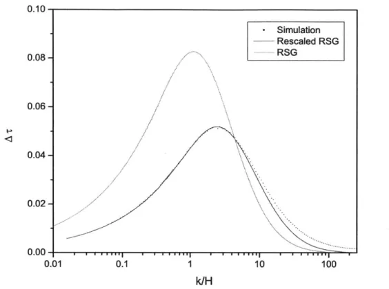
0.10 - Simulation Rescaled RSG 0.08- RSG 0.06 -0.04 -0.02 0.00-1 1 1 1.. il I a- rrr....I 0.01 0.1 1 10 100 k/H

Figure 3-1: Compare the RSG approximation with the Monte Carlo simulation. The

rescaling parameters are krescaled = 2,2k, ATrescaled = 0.63AT.

The bracket in (3.13) is the vacuum expectation, or in the simulation it is average over many different sets of random numbers.

3.3

Monte Carlo Simulation

As we have discussed in the previous chapters, the quantum fluctuations set the initial values at the top of the hill for the scalar field to roll down. Without the quantum fluctuations, the field would stay at the unstable equilibrium for an arbitrary long time. If we look at an arbitrary time-slice when the field is rolling down, the fluctuations are at the same order of magnitude as the field itself.

In our simulations, for each set of physical parameters, we run the simulation for

Table 3.1: Change the physical parameters p and pg, with fixed product pp+

for the vacuum expectation. As we can see in Fig. 3-1, the RSG approximation is at the same order of magnitude as the Monte Carlo simulation. Burgess has pointed out in her thesis that the RSG approximation would be in very good agreement with the simulation if we rescale AT and shift k, each by a factor of order 1. To find these rescaling factors, we first define a rescaled-RSG time delay field as a function with two parameters:

A-rescaled(k) = AArRSG(Bk) (3.15)

The total distance between this rescaled function and the simulation value can be calculated as

D(A, B) Z [Asimulation(k) - ATrescaled(k)]2 (3.16)

k

Then we will find the values of A and B such that D(A, B) is minimized.

To understand the behavior of the rescaling, we ran the simulation for a wide range of physical parameters m and mo. It turned out that the amplitude rescaling A was almost constant, stayed at 0.63 in the entire range of examined parameters, while the wave number shifting factor B was more sensitive to the physical parameters.

We also noticed that not only the rescaling factors, but also the peak of the time delay field and the time of ending inflation would be constant if we vary both two physical parameters pp and o, in such a way that their product is constant as in

Table 3.1. This can be explained as the mass dependence of the equation of motion for the mode functions

pg(1 - ePON) ~Op -iN + 2(pN)2 + --

)

(3.17)

pip pO A B 6Tmax tend

1/22 18 0.6280 2.203 0.052 12.79 1/33 27 0.6280 2.203 0.052 12.71 1/55 45 0.6280 2.203 0.051 12.68 1/110 90 0.6280 2.203 0.051 12.66

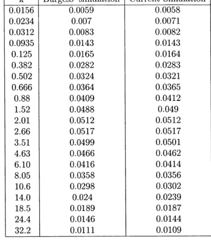
Table 3.2: Compare our simulation results with Burgess' for p = 18 and pp = 1/22. A B

[

6 rnax tend 0.450 0.629 2.821 0.0716 19.6 0.600 0.628 2.448 0.0617 15.9 0.818 0.628 2.203 0.0520 12.8 1.00 0.627 2.09 0.0460 11.1 1.28 0.626 1.982 0.0401 9.35 1.80 0.623 1.876 0.0331 7.45 3.00 0.620 1.770 0.0234 5.19 4.00 0.618 1.727 0.0192 4.24 5.00 0.617 1.704 0.0165 3.63 8.00 0.615 1.667 0.0120 2.63 11.0 0.614 1.649 0.00967 2.11 15.0 0.613 1.635 0.00784 1.71 20.0 0.613 1.628 0.00646 1.41 30.0 0.613 1.622 0.00492 1.07 50.0 0.613 1.614 0.00350 0.76

k Burgess' simulation Current Simulation

0.0156 0.0059 0.0058 0.0234 0.007 0.0071 0.0312 0.0083 0.0082 0.0935 0.0143 0.0143 0.125 0.0165 0.0164 0.382 0.0282 0.0283 0.502 0.0324 0.0321 0.666 0.0364 0.0365 0.88 0.0409 0.0412 1.52 0.0488 0.049 2.01 0.0512 0.0512 2.66 0.0517 0.0517 3.51 0.0499 0.0501 4.63 0.0466 0.0462 6.10 0.0416 0.0414 8.05 0.0358 0.0356 10.6 0.0298 0.0302 14.0 0.024 0.0239 18.5 0.0189 0.0187 24.4 0.0146 0.0144 32.2 0.0111 0.0109

is a function of pepp when N ~ 0. So the density perturbations are determined by the initial fluctuations of the field

#

at the time when the potential flips sign.

3.4

The Direct Integration Method

The Monte Carlo simulation can accurately describe the evolution of the scalar fied and evaluate the time delay. However, the amount of numerical work makes it ex-tremely difficult to expand to a realistic 3-dimensional system. In this section we will introduce a new method of evaluating the time delay field with excellent agreement with the Monte Carlo simulation in 1-dimensional system.

As we have discussed at the end of chapter 2, the equations for the asymptotic behavior of the mode functions were (1.28) and (1.29). So we can write

u(k, t --+ o) ~ eAtu(k) (3.18)

where A can be defined as

_ qrms(t )

A = rms(t) (3.19)

#rms

(t)

Then we have the approximate expression for the scalar field at late time is

I0(X7

t) 12 =

I0(X7

to) 12

e

2AHRt

(3.20)

where t = to + 6t and to satisfies

o2st) =#2, (3.21)

Solving for the time of ending inflation, we get

6t(x) = log (7 to)1) (3.22)

If we rescale the scalar field by its root mean square O(x, t) = -( t) then

OrMS (t)

1

of= 2A lg|~ ,t)2

We will evaluate the time-delay field in x space

(6t(x)6t(O)) = _ (log I (x, to)12log I (O, to)12)

where the bracket

()

denotes the vacuum expectation. Rewrite the complex scalar field as

O(x, t)

O(R, t) = X1 + iX2 = X 3+ iX 4 (3.25) (3.26)

where Xi's are real. The vacuum expectation can be written as the integration over the jointly Gaussian distribution of four random variables,

(F[X]) = d exp{ -- XTE-X}F[X]

1) J ~(2wr)2/detE 2 (3.27)

where

dX = dX 1dX2dX3dX4

Eij = (XiX,)

The mode expansion of the scalar field <(x, t) can be written as

X1 = 1N(x) + q*(x) 2 ) * X2t 14 x) - ($() 2iLJ (3.28) (3.29) (3.30) (3.31) (3.23) (3.24)

We can get the components of the matrix E as

1 1

Ell = ₌ E22 = ₌₂ -( (X) *(X)) = ₂

-E12= E21 = )+ q$*(

4i1

In the end, we will get the variance matrix as

2

z

0 A0 ₂1

x)q$*(x))

=

0

where

A = (X1X3) = (X2X4) = 1b

Ift(k,

to) 12eikx

and Equation (3.24) becomes _1 (6t(x)6(0)) =

4I

2

I

dX1dX2dX3dX4 log(X2 (27r)2[i - A2] g 1 exp{- 4[1 _ A2] [X + X 3+X X4 -+X) log(X2 + X4) 4(X1X3+ X2X4)A}

Changing the variables to polar coordinates

X,

=r 1 cos 01 X2 = rl sin 01 X3 = r2cos 02 X4 = r2sin02 (3.32) (3.33) (3.34) (3.35) iL(k, t) = u(k, t) Orms(t) (3.36) (3.37) (3.38) (3.39) (3.40) (3.41)

27r

127r

(6t(X)6(0)) = A2J do

d00

ridr 0 r2dr2 1

(27)2[i - A2]

exp{- 4 1 2 + r2 - 4Ar1r2cos]}

where 6 = 01- 02. Changing variables again

r = r4 r2 =)r equation (3.37) becomes log(ri)log(r₂) Cos sin

(6t(x)6(0))

= I 2- 7 (27r) [ 1- A2] A2 dO 17/2 d0 do cos

#

sin

#$

00

r3dr log(r cos log(r sin

#)

exp{- 1 - ₂ [r2(1 - 4A cos 0 sin 0 cos 6)]} (3.45)

The integration over r can be done analytically

00

r3dr log(ar) log(br) exp(-cr2₎

0

(

8

2 _{[ -} 2_{)- + - - 2 log ab(y - 1 + log c) + 4 log a log b + log c(2-y} - _{2 + log c)]}

(3.46) where a cos# b sinq# c 4 2 (1 - 4A os sin # cos 0) -y a0.577215664901532 then (3.42) (3.43) (3.44) (3.47) (3.48) (3.49) (3.50)

.,

, ,

0.1 1

- Monte Carlo Simulation Direct Integration

10

k/H

100

Figure 3-2: Compare the direct integration method with the Monte Carlo simulation.

The parameters are po = 18 and yp = 1/22. 0.06

0.04-

0.02-

-Consider the special case

(6t(0)6t(0)) = 4 2 27(l) exp{- X + X)} log2(X2 + X2) (3.51)

Changing variables lead to

(ot(0)Ot(0)) = dO

f

rdre-- [logr2]2

4A2 w

= 8 rdre-r2 [log r]2

= (,2 + 2)(3.52)

4A2 6

The integration (3.45) will give us the time delay field in x-space. The

corre-sponding k-space time delay field was plotted in Fig. 3-2 along with the Monte Carlo

simulation for reference. The difference between the two results is about 1%, which

can be think of as the limit of the convergence of the Monte Carlo simulation. It

would be possible to reduce the difference by increasing the number of runs in the

Monte Carlo simulation.

3.5

Variation of the time delay field

From the previous sections, we have seen that the both the time delay field and the mean ending time depend only on povg, but not po/pv,. Since we have investigated a wide range of physical parameters, it would be possible the see the pattern of the dependence. Define a new parameter as

POVO =(3.53)

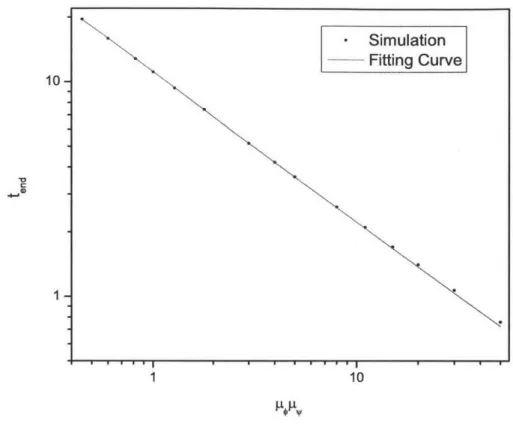
The dependence of the ending time tend and the time delay peak 6Tma, on ( can be

fitted as

- Simulation Fitting Curve

10-C

1 10

Figure 3-3: The mean ending time.

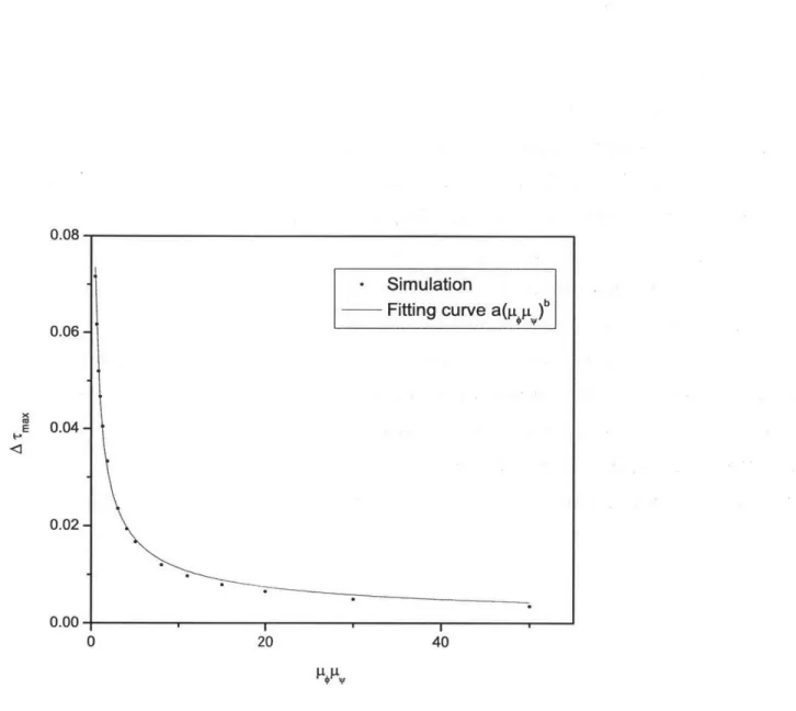
where a 0.045 (3.55) b ~ -0.60 (3.56) and tend(() = cd (3.57) where c 11.2 (3.58) d ~ -0.70 (3.59)

20 40

PLp

Figure 3-4: The peak of the time delay fields.

0.08

0.06

- Simulation

Fitting curve a(p p)

0

E

0.04-0.02

0.00 0

3.6

Conclusions

The time delay field calculated from the simple approximation proposed by Randall et. al. shows a very good agreement with that of the Monte Carlo simulation up to a rescaling in the amplitude and a shifting in the wave number both by factors of order

1. This is the same conlcusion as Burgess but with wider range of mass parameters po and p,. We also noticed that the time delay field only depends on the product

but not the ratio of the two mass parameters. By varying this product from 0.45 to

50, we can have the peak of the time delay field changing from 0.072 to 0.004.

The Monte Carlo simulation is a powerful tool to investigate the evolution of the fields in 1-dimensional systems, but very difficult to expand to 3-dimensional due to an enormous computational requirement. By integrating over the probability distribution of the scalar field, the direct integration method can accurately produce the result of the Monte Carlo simulation in the asymtotic regime when all mode functions increase with time at the same rate independent of k. The direct integration method is very suitable for 3-dimensional expansion since the probability distribution integration has the same form, with the only parameter dependence arising from the two point function A(x).

Bibliography

[1] T. S. Bunch and P. C. W. Davies. Quantum field theory in de sitter space: Renormalization by Point-Splitting. Proceedings of the Royal Society of London.

Series A, Mathematical and Physical Sciences, 360(1700):117-134, March 1978.

ArticleType: primary-article

/

Full publication date: Mar. 21, 1978

/

Copyright

1978 The Royal Society.

[2] Kristin Burgess. Early stages in cosmic structure formation. http://dspace.mit.edu/handle/1721.1/28643. Thesis (Ph. D.)-Massachusetts Institute of Technology, Dept. of Physics, 2004.

[3] Alan H. Guth. Inflationary universe: A possible solution to the horizon and

flatness problems. Physical Review D, 23(2), 1981. [4] Alan H. Guth. Notes for scalar field, 2001.

[5] Alan H. Guth and So-Young Pi. Fluctuations in the new inflationary universe. Physical Review Letters, 49(15), October 1982.

[6] S. W. Hawking. The development of irregularities in a single bubble inflationary

universe. Physics Letters B, 115(4):295-297, September 1982.

[7] Lisa Randall, Marin Soljacic, and Alan H. Guth. Supernatural inflation: inflation

from supersymmetry with no (very) small parameters. Nuclear Physics B,

472(1-2):377-405, July 1996.

[8] A. A. Starobinsky. Dynamics of phase transition in the new inflationary universe

scenario and generation of perturbations. Physics Letters B, 117(3-4):175-178, November 1982.