HAL Id: hal-03185047
https://hal.uca.fr/hal-03185047
Submitted on 30 Mar 2021
HAL is a multi-disciplinary open access archive for the deposit and dissemination of sci-entific research documents, whether they are pub-lished or not. The documents may come from teaching and research institutions in France or abroad, or from public or private research centers.
L’archive ouverte pluridisciplinaire HAL, est destinée au dépôt et à la diffusion de documents scientifiques de niveau recherche, publiés ou non, émanant des établissements d’enseignement et de recherche français ou étrangers, des laboratoires publics ou privés.
Approach 1
Yong He
To cite this version:
Yong He. Market transition in Rural China -A New Institutional Approach 1. EURASIAN JOURNAL OF ECONOMICS AND FINANCE, 2021, 3 (1), pp.1-21. �hal-03185047�
Market transition in Rural China –
A New Institutional Approach
1 Yong HeCERDI-CNRS, University Clermont-Auvergne, yong.he@uca.fr Received: 16 October 2020; Revised: 23 October 2020; Accepted 9 November 2020; Publication: 10 February 2021
Abstract: With the guidance of a framework of new institutional economics, the theoretical
modelling establishes the necessary and sufficient conditions for institutional change to occur in authoritarian regimes: first, external shocks must be strong, much stronger than in a democratic regime; second, the shocks must be of such a kind that gives rise to factional competition within the ruling group. It predicts that involvement by the ruled group brings about more extensive institutional change than that merely driven by the ruling group. The theory is then applied to explain rural China’s market transition. As institutional change defines payoff structure, the extent of this change is approximated by the income advantage of cadre households relative to noncadre households. Econometric tests based on a Chinese rural household panel data of 21 years confirm the theoretical prediction.
Keywords: Institutional change, authoritarian regime, political returns, market transition,
new institutional economics, Chinese rural cadre.
JEL Classification: B52, P2,R2. I. Introduction
Authoritarian regimes refer to political systems in which countries are ruled by a minor group of persons not chosenthrough voting process by the people. They correspond to all nondemocratic regimes, and coverabout one third of countries and onehalf ofthe population in the world.
This study adopts an approach of newinstitutional economics of which three Nobel prize owners: Ronald Coase, Douglass North and Oliver Eaton Williamson are the main contributors. Our theoretical framework is inspired by North’s analysis on institutional change in economic history. North (1992) has ever noticed the deficit of a newinstitutional understanding of non democratic world: “research in the new political economy (the new institutional economics applied to polities) has been largely focused on the United States and other developed countries. While we know a lot about the characteristics of the polities of third world countries we have very little theory about such polities”.
In North (1990)’s theory of institutional change, exogenous changes inthe environment (hereafter they are calledexternal shocks)alter relative prices, and organizations as player use their bargaining strength to reinforce or change the ongoing rules. Therefore, political competition between organizations is
the key condition for institutional change to occur. Applying this framework to authoritarian regimes, the crucial question to answer is how could exist politicalcompetition? If the ruling group monopolizes the decision makingaboutinstitutional change and their interests are more likely linked with the existing system, the status quo couldlast very long.
Ourmodel is grounded on following ideas.The players are divided into ruling and ruled groups in which only the first has decisionright forinstitutional change. The ruling group is assumed to beendogenously divisible into, using conventional terms, conservative and reformist factions.External shocks must bemuch stronger than in a democratic regime, because the ruled group is small in size, the common interest within the group is strong, and the costs for reaching an agreementare low. The strength of the shocks, nonetheless,is not the unique requirement.They must be of such a kind thatdifferentiates their interests, leading the reformists to perceive their advantages for engaging in institutional change, and making their bargaining strength to exceed that of the conservatives. Whenever the reformist faction is weaker than another one, institutional change is blocked.
Furthermore, institutional changejust coming from political competition within the ruling group is limitedin taking into accountthe interests of the ruled group. Involvement in institutional change by the ruled group itself is a major factor. This, again, depends on the strength and nature of external shocks. Some types of shocks could affect relative prices to the advantage of the ruled group. The best example is the Black Death in Europe during 14th century that caused sudden wage increase. As the results of these shocks, individual choices and actions in consumption, production, and other activities could make ongoing institutional setting obsolete. This involvement firstly contributes to the decision making on institutional change by the ruling group throughreinforcing the bargaining strength of the reformists within the ruling group. It also gives rise to more extensive institutional change than the one merely driven by intraruling group competition.
Therefore, the necessary condition forinstitutional change in authoritarian regimes is strong external shocks. The differentiation between the interests of the conservative and reformist factions within the ruling group and their competitionarethe sufficient condition for this change.Furthermore, the degreeofpopularinvolvementdetermines the extent of this change.
This theory is testable, first through empirical validation with case studies, and second with econometrical tests. We explain China’s rural market transitionwith this theory throughdividing this transition into three phases. External shocks haveprompted all of them. Whereas the first two phases were driven by the political competition within the ruling group, the third proceeded with strong involvement by the ruled group through their voting by feet.
Then we set an econometric test for verifyingthe prediction that with popular involvement, institutional change ismore extensive than that merely
driven by the ruling group. Given, following North, an institutional change defines changes in payoff structure, and this structure has two dimensions: overall growth of the payoff and its distribution among individuals, we are able to use global income growth and political returns reflecting income distribution among ruling and ruled groups as indicators to measure the extent of institutional change. Political returns are specific to authoritarian regimes, because in the absence of democracy, these returns correspond to the rents resulting from the monopoly of the ruling group.These returns must be changing along with institutional change that affects the power to control of the group. Asample of household panel data from 1989 to 2009 is constituted, and political returnsare defined as the ratio of the net income advantage of cadrehouseholdsto the incomes of noncadre households.Applying fixed effects and matching method to minimize estimation bias, we find that, as expected, the third phase brought about much higher income growth as well assharperdecrease in political returns.
To summarize, this study has contributed to: 1) constructing a theoretical framework to explain the blockage and occurrence of institutional change in authoritarian regimes; 2) empirically illustrating the theory with Chinese rural market transition and providing econometric teststo the key theoretical prediction.The study, therefore,has filledthe gap of the new institutional theory in the deficiency of theoretical setting and empirical tests on institutional change in authoritarian regimes.
The remainder of this study is organized as follows. Section II constructs the theoretical framework. Section III applies the theory to analyzeChinese rural market transition. Section IV provides arguments for the measurement of the extent of institutional change, introduces data and econometric methods, and analyzes the results. Finally, section V concludes.
II. The theory
Bad institutional change happens more frequentlyin authoritarian regimes.In this study, however, institutional change, like in most previous works,implicitly refers to “good” institutional changethat, in broad sense, leads to Pareto efficiency.
North (1990, 1991) provides a general economic approach to institutional change. Institutions define the rule of the game and the payoff structures. External shocks arethe driving force of institutional change through altering relative prices, and creatingopportunities for the players in the society to change the rules of the game; Organizations are players. They consist of groups of individuals bound together by some common objectives, andcompete in function of the perceived advantages and costs of altering the institutional framework.Institutional change comes as the result of their competition.
Applying this approach to authoritarian regimes, as a large majority of people are excluded from the decisionmaking process, political competition
appears absent. North (1996) puts major importance on political competition, and affirmed that the best political solution is democratization in which, political market reaches to a solution at the lowest transaction costs.
In following model,we show that, together with some other mechanisms, political competition similar to democratic competition exists in authoritarian regimes in a special form.
II.1. Political competition within the ruling group
In authoritarian regimes, the competition between different factions within the ruling groupbecomes possible because the composition of the group is not homogenous (for an analysis on communist regime, cf. He, 1992). Adopting the most conventional way, its members can be distinguished into reformist and conservative factions: the former is more likely to accept and the latter refuseinstitutional change. Note J as the decision rule for an institutional change:
J = R – C (1)
J is a function of bargaining strengths of the reformist faction R and the
conservative faction C. Institutional change is blocked if J � 0. Otherwise the change passes.
Bargaining strengthsof the two factions are function of the extent and kind of external shocks, or, the formation of two factions is endogenously determined. We firstly specify three effects of external shocks:
PR = f(E)
where E refers to the extent and kind of externalshocks, and PR the relative prices effect in the favor of the reformist faction to the detriment of the conservative faction, with �PR/�E being either > 0 or � 0. In the latter case, the conservative faction is more favored.
In the context of developing countries in which authoritarian regimes are more likely to subsist, people potentially belonging to reformist faction arethose with higher education level and entrepreneurial ability. One example of this relative prices effect is that the appearance of new technologies could valorize the ability of the technocrats.
A tax revenue effect is also assumed, which refers to a potential change in tax revenue for the governmentwith thenew institutional settingsas the consequence of external shocks relating to this revenue under the old one:
T = f(E)
where T is the estimated tax revenue change, with �T/�E being either > 0 or ��0. The political stability, defined as the propensity for the change of political regime, is also a concern:
S = f (E) (4)
where S reflects the change in political stability level with the new institutional settings as the consequence of external shocks relative to this level under the
old one, with �S/�E being either > 0 or ��0. New institutional setting often threatens political stability, thus increases the bargaining force of the conservative faction.
Combining these equations, and assuming that the reformists care changes in tax revenue, and the conservatives in political stability, we get:
J = R[PR(E), T(E)] – C[PR(E), S(E)] (1.1)
where R� > 0 and C� < 0.
R� > 0 means that relative price and tax revenue effects favor the reformist faction. Whenrelative prices change provides the opportunity for some members of the ruling group to gain under a new institutional setting, and the gain is enough large to reach a Pareto efficiency (that is, the gain is always positive after recompensing the potential losers), the reformistsbenefit from a rise in bargaining strength. Likewise, tax revenue effect also reinforcesthe bargaining power of the reformists,because they bring improved governmental financial conditions. C��< 0 can be interpreted in a similar way: a threat topolitical stability reinforces conservatives’ bargaining strength.
Equation (1.1) implies that the existence of strong external shocks is a necessary condition for institutional change. Just like in a competitive product market in which prices are highly sensitive to slight adjustment between supply and demand,in a democratic regime, the political market insures that even a weak shock altering relative prices could spontaneously yield a demand for institutional change.In authoritarian regimes, however, as the costs of an agreement reachedwithin a smallsized group are small, andas the maintenance of their rule is a strong common interest, in the presence of weak shocks, the ruling groupis more likely to keep unified, and blocks institutional change.
Equation (1.1) also implies that the existence of strong external shocks is only a necessary condition. J > 0 not only requires E being enough strong, but also, �PR/�E > 0, �T/�E > 0 and external shocks havingweakpolitical stability
effect (the absolute value of �S/�E is low). In other words, the occurrence of
institutional change also depends on the kinds of external shocks. Some kind of shocks, albeit strong, may fail to differentiate the interests of the two fractions trough PR, T and S. In this case, institutional change could be blocked. Therefore, the occurrence of factional competition is the sufficient condition for institutional change to takeplace.
II.2. Involvement by the ruled group
By definition, the members of the ruled group are excluded from decisionmaking. By which mechanism they are able to be involved in institutional change? Again, external shocks play a crucial role.
Note A the degree of involvement by the ruled group, which is affected by the shocks via changes in relative prices in the favor of the ruled group (PA):
A = f(PA (E)) (5)
While some kinds of shocks differentiate the interests of the ruling group, the others create changes in relative prices in the favor of the ruled group. In subsequent Chinese case, globalization stimulating a rise in wage of rural workers is an example.
When external shocks make actual payoff structure defined by ongoing institutional setting inacceptable for most population, given political voting is unavailable, various processes emerge to fulfil similar function. By involvement from the ruled group, we refer to all kinds of actions, going from changes inindividuals’ choices in consumption and production to political manifestations that express their discontent and weaken existing institutional setting. In rural China’s case, the best example isthe “voting with feet”, or leaving rural regions for cities where the treatment is better, which meaningfully reduced the realm of control of the ruling group. Another example isthe prevalent absenteeism and nonchalance during work that caused huge inefficiency in ExSoviet economy. The actions oftrade unions or of other organizations authorized in some autocratic regimes also give rise to these effects.
Another role of popular involvement is its influence over the ruling group via changes in tax revenue: The demand for institutional change by ruled group, if satisfied, could increase tax revenue, and enhance the bargaining strength of the reformist faction. Or:
T = f(A) with �T / �A ��0 (6)
On the other hand, popular participation in institutional changemay also cause ruling group’s concern aboutpolitical stability:
S = f(A) with �S / �A ��0 (7)
To simplify,the effect of popular involvement on tax revenue and on politic al stability can be inc luded in T(E) and S(E) of Equation (1.1)respectively, so that in the presence ofpopular involvement, the decision rule is always defined by Equation (1.1), but with the awareness that the terms T(E) and S(E) are different between the cases with or without popular involvement.
The key role of popular involvement is that institutional change, whenever decided by the ruling group, will become more extensive than that merely driven by the ruling group. In authoritarian regimes, institutional change mostly consists in giving up some control power by the ruling group in the favor of individual freedom of choice. This concession made merely as the result of the compromise within the ruling group must be smaller than that achieved under the pressure of popular involvement.
Note V as the extent of institutional change. Without popular involvement,
V = f(R, C) with �V/�R > 0, �V / �C < 0; V = 0; if R – C ��0 (8) With popular involvement,
V = f(R, C, A, �RA, �CA) (9)
�RA and �CA are respectively induced bargaining strengths of reformist and conservative factions derived via Equations (6) and (7).In other words, in the absence of voting right, popular involvement also contributes to the decision making on institutional change.
With popular involvement, institutional change is biggerif:
A + �RA > �CA (10) In general, this condition holds, because the ruled group is numerically important, leading popular participation to change the balance of bargaining forces. Nevertheless, it is always possible that the concern forpolitical stability leads �CA to be so high that R + �RA� C + �CA, or institutional changeis blocked. This extreme case often happensinpolitical institutional change. In other cases, especially in the case of economic institution reforms, �CA due to the concern to political stability should be at a reasonable level. Therefore, the condition defined by Equation (10) is more likely to hold, leading institutional change with popular involvement to be larger than that merely driven by within ruling group competition.
II.3. The achievability of institutional change
As the result of foregoing analysis, the conditions under which institutional change is achievable or blocked can be set out.
External shocks could be either neutral or alter relative prices. In the former case, there could be no influence oninstitutional change. In the second case, the influences depend on 1) if they affect relative prices that differentiate the interests ofruling elites or are in the favor of the ruled group; 2) if they exert tax revenue effects. Fully expressingthe extent of institutional changeas a function of external shocks, we get:
V = f{R[PR (E), T(E)], C[PR (E), S(E)], A[PA (E)]} (11) Logically externalshocks are also able to cause bad institutional change ifall or some of the derivatives: �PR / �E, �T / �E, and �PA / �E are negative, so
that �V / �E < 0. But we only consider the case where V � 0.
On the basis of Equations (1.1) and (11), we are able to identifyfivetypical cases summarized in Table 1.
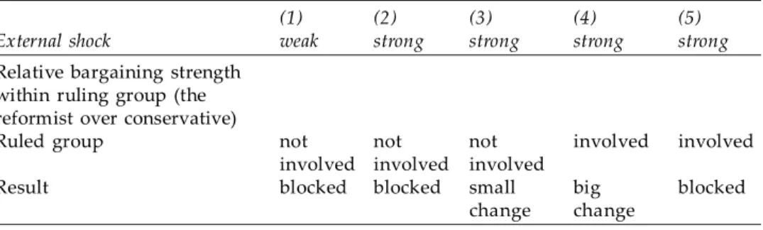
Table 1: A typology of institutional change
(1) (2) (3) (4) (5)
External shock weak strong strong strong strong
Relative bargaining strength within ruling group (the reformist over conservative)
Ruled group not not not involved involved
involved involved involved
Result blocked blocked small big blocked
change change Source: author.
Case 1: When external shocksare weak, so that J � 0, there is not any institutional change.
Case 2: The shocks are strong buttheir effects on relative prices and on tax revenue are quite weak (some or all of �PR / �E, �T / �E, and �PA / �E are small),
or the concern forpolitical stability is too strong (the absolute value of �S / �E
ishigh) so that J � 0, there is not any institutional change.
Case 3: Institutional change occurs with �PR / �E > 0, �T / �E > 0), small
concern about political stability, and absent popular involvement (�PA / �E =
0), so that �V / �E > 0. The extent of the change is small (V is small).
Case 4: Other things being equal to Case 3, there is in addition popular involvement (�PA / �E > 0), so that not only �V / �E > 0 (institutional change
occurs), but alsothe extent of change is large (V is large).
Case 5: Other things being equal to Case 4, there is a big concern for political stability (S(E) is high in absolute value), so that J � 0, institutional change is blocked.
III. An application to Chinese rural market transition
Market transition is a typical case of institutional change. Chinese rural market transition proceeded in a context of change from collectivist command economy to market economy. Rural cadres,officials working in townships and villages, played a leading role in this transition. They form the base for rural political and economic governance,and constitute the ruling group.Statistic information on rural cadres is scarce.They are estimated to be about1.5% of rural population.2
Three phases of Chinese rural market transition can be distinguished, and their differences can be analyzed with the key factors derived from our theoretical framework: external shock, political competition within the ruling group, and the degree of popular involvement.
First phase (19781996) was the establishment of the household responsibility system (HRS). Collective land ownership kept unchanged, peasants were contracted to explore a certain size of land during 30 years renewable, and the yields beyond the quota was sold in free markets at unregulated prices. Thrusted by this change, there was a large development of the township and village enterprises (TVEs).
The external shockdriving this change was the economic crisis caused by the Cultural Revolution (19661976), in which uninterrupted political struggles made national economy to reach the brink of collapse. More incentive rural production system was called for going out from the crisis. This was an external shockcoming from urban area to rural region.
This was a cadredriven institutional change. Theshock altered relative prices in the favor of one part of cadres with higher education level and entrepreneurial ability. The naissance of TVEs started during the mid1970s. Since then alarge number of cadres were formed to be business managers.
While the conservative faction saw loss of control in land and other resources, the reformists got more advantages from the expansions of TVEs,a natural consequence of the application of HRS, which derived important surplus labor. The reformist cadres also benefited fromexpandingtrading networks owing to the growths of TVEs and of agricultural production.
The involvement by peasants, the ruled group,was limited. Without the permission by cadres, peasants had not any right on how to use lands and organize productions, and only passively adapted to this change and accepted their role assigned by cadres.
It is noteworthy that in China, institutional change often proceeds in a form of “ex post institutionalization”. The reform starts at firstin small scope, sometimes clandestinely. If producing positive results, it will be extended to other zones, and at last recognizedofficially. Otherwise, it will shrink in sizeand disappears. The emergence of HRS was in Xiaogang village. After having suffered a severe drought, 18 households secretly signed a contract with local cadres to be allocated lands for exploration, a methodstrictlyforbidden under the old system. In 1979, similar experiments were launched and expanded in Sichuan and Anhui provinces, and generateddramatic increase in agricultural productivity. In 1981, the central government openly praised the reform, and new system was adopted nationwide .
With this change, quickly cereal and food shortage disappeared, and rural industrialization started. Between 1982 and 1988, industrial output of TVEs grew at an average annual rate of 38.2% (Putterman 1997). In the end of this phase, TVEs produced over 30% of all China’s industrial added value, profit and output, and all TVEs across nonagricultural sectors created more than 15% of China’s GDP (Sun 2002).Correspondingly, employment in TVEs rapidly increased to reach to 125.37 million in 1998.
The second phase (between1997and2000, extendable to 2003) was marked with the privatization of TVES. The East Asia economic crisis in 1997 suddenly reduced market size for TVEs adopting laborextensive technology. Market competition had constrained the ability of TVEs to meet revenue and employment imperatives, while local governments’ salesoriented growth strategies had exacerbated governance problems (Kung and Lin 2007). In response to this decline, many small TVEs in financial difficulties were asked either to close or privatized. Thistrend of privatization can be estimated to reach itsend by 2003 where most TVEs had been ownedby private majority shareholders.
Following the theoretical model, again, the success of privatization was due to an external shock: the East Asia crisis, which placed intensive pressure forthe ownership change. More importantly, this shock made the relative prices of entrepreneurial ability appreciated. The Party technocratshad strong incentive for the change in ownership because it could bring enormous benefits to them. According to Li and Rozelle (2003), local governments almost always
sold firms to insiders, especially to their managers or other private owners closely linked with local officers in largescale TVE ownership restructuring. Therefore, this wasalso a cadreled institutional change. The big winner of the privatization was a number of cadres. Peasants had neither opportunities nor capital to be the owners of TVEs, and for them there was little difference between working in collective and privateowned TVEs.
The process of privatization, once more, went in the way of ex post institutionalization. At first privatization started locally and clandestinely, then, at last, it was generalized and formally recognized.
The third phase started from 2000, and was featured by the acceleration ofruralurban migration.According tothe Statistic Annual Yearbooks,the share of migrant workers in total rural labor increased from 7.14% in 1990to 19.47%in 2000. This share reached to 30.91% in 2005 and to 56.17% in 2010.
Eexternal shock came from China’s integration into globalization. Since 2000, as major providers of a large number of manufacturing goods, Chinese coastal regions had been enjoying the reputation of the “world factory”. The increase in demand and in wageincited morepeasantsto leavetheir villages and to work in cities. Ruralurban migration was thentightly restrained by a system of household registration (the Hukou system) with discriminating conditions for rural workers on food quota, housing, medical care, child schooling, and employment (Young 2013).Rural workers were administratively
kept in their villageswithout right of free movement. Before,with less attractive wage
and high costs for installing in cities, staying in villages was the privileged choice for most farmers. With this shock, a massive increase of rural migrants can be considered as voting with feet against ongoing institutional setting in the disfavor of peasants.
This phase also marked a profound evolution in the way of institutional change. It was no longer, as in earlytwo phases, driven by cadres, but by peasants themselves. External shocks made peasants individually changed their choices in allocation of labor. These individual actions produced a collective effect, which made a mounting pressure on the ruling group to reconsider their institutional setting. To satisfy the increasing demandforlabor in cities, the loosening of restrictions on migration came also in a way of ex post institutionalization.It started infew provincesin need ofmigrant workers. It was until 2014 that the differentiation between agricultural and non agricultural Hukou statuses was definitively suppressed at the national level. Three remarks can be made from the comparison of three phases. First, they constitute a whole process of market formation. The first phase partially formed land and products markets. Since then peasants were allowed to rent their contracted lands to the others, and to sell their products. The second phase marked the nascent form of capital market following the privatization of TVEs. Finally,the third phase formed the labor market in which labor mobility became possible.
Second, while two first phases were cadredriven institutional changes, the third was thrusted with intense involvement by peasants.
Third, not only external shocks were needed to be strong, but also successive for the success of market transition. Moreover, because external shocks exerted different relative prices effects: those favorable to reformist cadres and those to peasants, institutional change was driven only by cadresduring the first two phases, whereas peasants were involved in the third phase.
IV. Empirical Tests
The theory mainly yields two predictions: 1) the occurrence of strong external shocks is a necessary and factional competition within the ruling group a sufficient condition for institutional change to take place; 2) institutional change is bigger with popular involvement than that merely driven by the competition within the ruling group.Case studies with descriptive statistics are able to verify the first prediction. This section showswhy and how the second prediction is testable.
IV.I. The measurement of institutional change
The test of the second prediction requires quantitatively measuring the extent ofan institutional change. Following North, institution defines payoff structure. Consequently, a more extensive institutional change must induce bigger change in payoff structure. The change in payoff structure has two dimensions: the growth of total payoff and the change in its distribution among individuals, especially between the people belonging to the ruling and ruledgroups. In the context of rural China, globalin come growth rate corresponds to the first dimension, and changes in political returns, as will be shown, can measurethe payoff distribution. With these indicators, it becomes possible to verify the prediction that the third phase with popular involvement brought about institutional change bigger than that during the first two phases.
Political returns can be defined as the ratio of the net gain from one unit of investment in political activity to its opportunistic costs in other activities. These returns can be surrogated by the ratio of the advantage in income of the ruling group to the income of the ruled group. Political returns are higher in authoritarian regimes, because these returns correspond to the rents derived from the monopolistic political position of the ruling group. The more powerful the monopoly, the higher political returns will be.
A handful of work has addressed political returns. Fisman (2001) showed that in every case of the emergence of a string of rumors about the health of former Indonesian President Suharto, the returns on shares of politically dependent firms were considerably lower than the returns of lessdependent firms. Goldstein and Udry (2008) provided evidence that in Ghana, individuals
holding powerful positions in local political hierarchies have more secure tenure rights to cultivated land and enjoy substantially higher output.
Nee (1989) affirmed that during a transition from planning to markets in rural China, there may have been diminishing political returns. This is because in a central planning system, with economic resources concentrated in the hands of political officials, returns to political power and status must be high. Market transition signifies a progressive change to acompetitive income determination, leading to decreasing political returns of them.
Following our theory, the trend of political returns may not emerge so unidirectional. First, political returns could be not decreasing because the ruling group has the possibility to block market transition. Second, political returns can be either no decreasing or periodically increasing if the payoff structure of a cadredriven transition is excessively to cadres’advantage. Only with popular involvement, institutional change could be expected to producedecreasing political returns. Subsequent section will focus on how to test this predictionempirically.
IV.2. Data and Estimating methods
CHNS database is constituted with longitudinal surveys of eight waves (1989, 1991, 1993, 1997, 2000, 2004, 2006, 2009 and 2011).3 The surveys cover more
than 30000 individuals from about 8000 households (about twothirds from rural and onethird from urban populations) in nine representative Chinese provinces.
Cadre households are defined as the households with at least one member being village or townshiplevel cadres. According to our estimation, the share of cadre households in total rural households is around 5% in rural China.
608 cadre households are identified, in which at least one of household members were reported as a cadre in one of waves 1989, 1991, 1993, 1997 and 2000 in rural areas. As the Chinese government is vigilant on political topics, data on this issue is unusually incomplete. Some cadre households may deliberately not report the existence of cadres. To deal with this, the strategy adopted in this studyis to consider all households that reported at least one time the existence of a cadre as cadre households. The year of their reporting is the starting year, and their cadre household status is assumed as lasting to the final wave of their participation in survey.
Since some cadres, after one or several mandates, may quit their posts,could this way to deal with the data incompleteness lead to serious bias? Several arguments suggest overlooking the effect of this measurement error. First, as cadre is a stable and relatively high profit job, cadres in active service have an incentive to keep their posts as long as possible. Second, the absence of elections favors the reigning cadres to keep their posts by themselves or their relatives. Third, as most cadres must first be Party members, and Chinese rural areas and populations are large, the ratio of Party members to population is much
lower than in urban areas.4 In most villages, a smallnumber of households
with Party members constitute a closed choice set for cadre nominations.5
Fourth and more importantly, becoming a cadre is an investment, or an establishment of a social network. The engagement in political activities forms an accumulative capital. Even after resignation, excadres still exercise influences in village or township activities. Therefore, the absence of formal title could have limited effects on their returns.
As we need to observethe evolution of income effects, among 608 cadre households, a number of them only appeared in a short period due to their interruptions in survey. Arbitrarily the study only keeps those that lasted at least four waves (at least 9 years). As such, 429 cadre households are kept, with 2608 observations.
To ensure comparability, first are removed the noncadre households, of which survey waves started in 2004, 2006 and 2009 due to their limited lengths. Then are removed all households that did not participate in all surveys from their starting wave to wave 2009. This way, 1911 noncadre households are kept for comparing with 429 cadre households. Thus, the panel data set is a total of 2340 households and 16062 observations, starting from waves 1989 to 2000 and ending to wave 2009.
As the first task, we define political returns as
t t c nc t t nc Y Y Y in wave t,
where Y and Ct Y are respectively incomes of household with and withoutnCt
political cadre.
Previously a number of workhave explored the existence of the returns to being cadres and variables explaining these returns in rural China (e.g., Parish et al. 1995; Nee 1996; Parish and Michelson 1996; Cook 1998; Morduch and Sicular 2000; and Walder 2002). These studieswerequerieddue toselection bias they encountered: If rural cadres are richer not because they are cadres, but because of some unobservable superior capabilities, and their becoming cadre and their higher income are both explained by these capabilities, the conclusion that they are rich because of their cadre status would not be fully convincing. In this case, econometrically, both explanatory and dependent variables correlate with error terms, and endogeneity leads to biased estimates.
Before the presentation on how to deal with the selection bias, we list all variables contained in econometric tests.
State_job, collective_job and private_job are three most important income
sources of Chinese rural households. Leaving_home is used to identify the effect of household’s financial resources coming from members working in cities. It affects income in two ways: labors working outside through remittance could raise income. They may also reduce income if they devote income for residing in cities (e.g., housing purchasing). Age, Age2, Gender and Education,used here as control variables, are variables reflecting the household human capital.
Estimations are made with following equation: 4 4 8 2 1 1 1 2 ( * ) it k k ik l l il t t t i jt it Y X Z C Wave µ Wave (12)
The dependent variable, Yit, is Income for household i in year t. Xk is one of
the explanatory variables. Zl is one of the control variables. All these variables are defined in Table 2. Wave is a time dummy between 1989 and 2009, in a total of 8 time points. Variable C is cadre household dummy. As C is timeinvariant and in fixedeffects models timeinvariant variables cannot be estimated, the cross products of cadre household dummy and Wave are used to capture cadre households’ income advantages over time.6 Therefore the coefficient of interest
is �t. Unobservable household characteristics such as ability, family background and other intangibles are captured in µi. Since in fixedeffects models, time invariant variables cannot be estimated, province cross wave is used to control for province fixed effects (�jt). Lastly, �ijt is the error term.
To address the selection bias, this study explores two econometric methods. First, the fixedeffects models are employed. Householdlevel fixed effect models have an advantage to partially overcome endogeneity and selection biasby using fixed effects terms µi and the province fixed effects �jt. Also in household panel data, the serial correlation between the withinhousehold error terms is a concern and this autocorrelation over time biases the t, F and
R2 values. To correct this, White Standard errors clustered at the household level are used throughout.
Second, among 1911 noncadre households, a matching method is applied to identify a group of noncadre households that were as similar as possible to
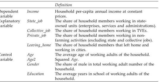
Table 2: Variable definitions Definition
Dependent Income Household percapita annual income at constant
variable prices.
Explanatory State_job The share of household members working in state variable owned units (enterprises, services and administrations).
Collective_job The share of household members working in TVEs. Private_job The share of household members working in non
farming activities (excluding state and collective jobs). Leaving_home The share of household members that left home and
working in cities.
Control Age The average age of working adults of the household.
variable Age2 Squared Age.
Gender The share of male in total working adult number of the household.
Education The average years in school of working adults of the household.
Notes: 1) Data come from the CHNS database.2) All explanatory variables are scaled by the number of household working adults, defined as household members over 16 years old.
the cadre household group at the starting time of evaluation. The procedure is to match the treated and untreated individuals according to their observable characteristics with propensityscore matching methods (See Cameron and Trivedi 2005, chapter 25).
For this purpose, percapita income, asset, education, mean age of adults, and household size are used to identify the matching group.7 They are the
noncadre households whose propensity scores fell within the range of scores of the cadre household observations. Finally as matching the households in the regions with similar development level makes sense, matching was separately appliedin three regions: Coastal, Central and Western regions.8 This
way, a data set of 429 noncadre households with 2801 observations is constituted. Coordinately, there are 1482 nonmatched noncadre households with 10653 observations.
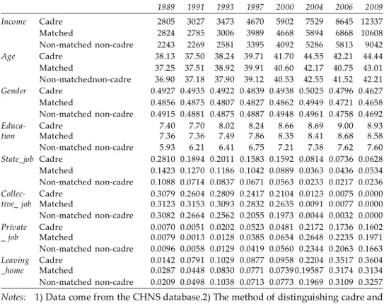
Table 3 presents the evolution of mean values of all variables over time by cadre household group, matched noncadre household group, and non matched noncadre household group.
Table 3: Mean values of variables by cadre and noncadre households
1989 1991 1993 1997 2000 2004 2006 2009 Income Cadre 2805 3027 3473 4670 5902 7529 8645 12337 Matched 2824 2785 3006 3989 4668 5894 6868 10608 Nonmatched noncadre 2243 2269 2581 3395 4092 5286 5813 9042 Age Cadre 38.13 37.50 38.24 39.71 41.70 44.55 42.21 44.44 Matched 37.25 37.51 38.92 39.91 40.60 42.17 40.75 43.01 Nonmatchednoncadre 36.90 37.18 37.90 39.12 40.53 42.55 41.52 42.21 Gender Cadre 0.4927 0.4935 0.4922 0.4839 0.4938 0.5025 0.4796 0.4627 Matched 0.4856 0.4875 0.4807 0.4827 0.4862 0.4949 0.4721 0.4658 Nonmatched noncadre 0.4915 0.4881 0.4875 0.4887 0.4948 0.4961 0.4758 0.4692 Educa Cadre 7.40 7.70 8.02 8.24 8.66 8.69 9.00 8.93 tion Matched 7.36 7.36 7.49 7.86 8.35 8.41 8.68 8.58 Nonmatched noncadre 5.93 6.21 6.41 6.75 7.21 7.38 7.62 7.60 State_job Cadre 0.2810 0.1894 0.2011 0.1583 0.1592 0.0814 0.0736 0.0628 Matched 0.1423 0.1270 0.1186 0.1042 0.0889 0.0363 0.0436 0.0534 Nonmatched noncadre 0.1088 0.0714 0.0837 0.0671 0.0563 0.0233 0.0217 0.0236 Collec Cadre 0.3079 0.2604 0.2809 0.2417 0.2104 0.0123 0.0075 0.0000
tive_ job Matched 0.3123 0.3153 0.3093 0.2832 0.2635 0.0091 0.0077 0.0000 Nonmatched noncadre 0.3082 0.2664 0.2562 0.2055 0.1973 0.0044 0.0032 0.0000 Private Cadre 0.0070 0.0051 0.0202 0.0523 0.0481 0.2172 0.1736 0.1602 _ job Matched 0.0079 0.0013 0.0128 0.0385 0.0654 0.2648 0.2235 0.1971 Nonmatched noncadre 0.0096 0.0058 0.0129 0.0419 0.0560 0.2344 0.2063 0.1663 Leaving Cadre 0.0142 0.0791 0.1029 0.0877 0.0958 0.2204 0.3517 0.3604 _home Matched 0.0287 0.0448 0.0830 0.0771 0.0739 0.19587 0.3174 0.3134 Nonmatched noncadre 0.0209 0.0498 0.1038 0.0713 0.0773 0.1969 0.3109 0.3257
Notes: 1) Data come from the CHNS database.2) The method of distinguishing cadre and noncadre households is introduced in this section.3) The constitution of matched noncadre household group is made with propensityscore matching methodintroduced in this section.
These descriptive statistics provide some interesting information.First, as expected, the cadre group hadthe highest,and the nonmatched noncadre group had the lowest incomes. The gaps in income between cadre and matched noncadre households were smaller. Wave 2009 appeared to be a “bound” in terms of income growth. Through checking, it was found that between 2006 and 2009, there were a significant number of households that began to generate profits from businesses, and this meaningfully influenced the mean income of the population.
Second, while differences in age and gender were not significant, cadre group had net superiority in education over nonmatched noncadre group. This gap between cadre and matched noncadre groupswas small.
Third, in most waves, while cadre households’ share of employment in state owned units was higher, the differences in collectiveowned units between cadre and noncadre householdsvaried in periods. Theshare of the cadre households in private nonfarm businesses, however, became lower than that of noncadre households since 2000. Over the period, jobs in stateowned and collectiveowned units decreasedprogressively to the benefit of private businesses. This corresponds well to above analysis on market transition process.
Finally, leaving home and working in cities were increasing so that in 2009, in all three groups, about one third of the working force left home.
VI.3. Results
Table 4 contains two regressing results basis on Equation (12). The values of
R2 are all satisfactory. F statistics are significant. The rho values are over 0.3. As the group variable is the household, high rho value signifies strong individual effects of households, indicating the appropriateness of the fixed effects models.
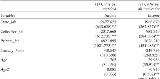
Table 4: Fixedeffects regression results
(1) Cadre vs. (2) Cadre vs. matched all noncadre
Variables Income Income
State_job 2477.623 1968.870 (643.638)*** (362.837)*** Collective_job 2017.668 982.340 (612.735)*** (284.586)*** Private_job 4821.895 3626.210 (1021.773)*** (451.085)*** Leaving_home 40.547 249.786 (518.588) (260.925) Age 11.705 79.986 (84.454) (35.914)** Age2 0.085 0.943 (0.853) (0.362)*** contd. table 4
Education 287.501 191.250 (117.549)** (61.097)*** Gender 1667.032 1886.149 (966.438)* (452.159)*** Cadre_1991 272.303 176.020 (433.914) (280.428) Cadre_1993 204.495 177.419 (451.686) (302.866) Cadre_1997 711.666 800.800 (478.947) (328.110)** Cadre_2000 1367.238 1178.260 (527.565)*** (364.312)*** Cadre_2004 1762.362 1918.262 (583.378)*** (436.855)*** Cadre_2006 1907.372 2448.593 (780.450)** (510.057)*** Cadre_2009 1579.319 2776.965 (962.046)* (683.926)***
Wave_dummy yes yes
Province wave yes yes
Constant 1802.668 2098.986 (2396.885) (985.105)** Observations 5409 16062 Household number 858 2340 Rsquared Within 0.2374 0.2180 Between 0.2423 0.2452 Overall 0.2435 0.2306 F (prob>F) 11.68 27.58 (0.000) (0.000) Rho 0.3250 0.3120
Notes: 1) Data come from the CHNS database.2) The method of distinguishing cadre and noncadre households is introduced in section IV.2.3) The constitution of matched noncadre household group with propensityscore matching method is introduced in section IV.2. 4) The regressions are made based on Equation (12). 5) Robust standard error is in parenthesis.6) * p<0.10; ** p<0.05; *** p<0.01.
The sample of the firstregressioncontains cadre group and matched non cadre group. That of the second regression contains cadre group and all non cadre groups. Based onthe previous arguments, the first estimation isdeemed having less estimation bias than the second one. We focus on the coefficients of cadre dummy over time from cadre_1991 to cadre_2009, with cadre_1989 as the base line. The coefficients of cadre dummy generally confirm the existence of income advantage of the cadre group over time.
In table 5, political returns measured as
t t
C nc
t nc
Y Y
t C
Y and Y are respectively incomes of household with and without politicalnct
cadre in wave t. In line “mean”, these returns are computed with the mean values of incomes of different groups contained in Table 3. In line “estimated”, the term t t
c nc
Y Y is replaced by the estimated coefficients from cadre_1991 to cadre_2009 derived from Table 4.
Table 5: The evolution of political returns
1989 1991 1993 1997 2000 2004 2006 2009
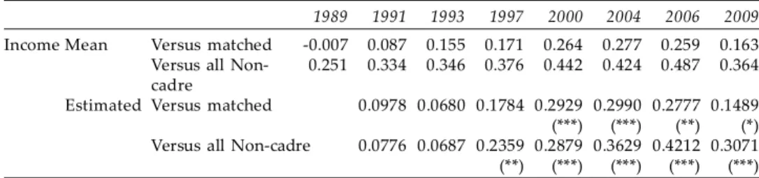
Income Mean Versus matched 0.007 0.087 0.155 0.171 0.264 0.277 0.259 0.163 Versus all Non 0.251 0.334 0.346 0.376 0.442 0.424 0.487 0.364 cadre
Estimated Versus matched 0.0978 0.0680 0.1784 0.2929 0.2990 0.2777 0.1489 (***) (***) (**) (*) Versus all Noncadre 0.0776 0.0687 0.2359 0.2879 0.3629 0.4212 0.3071 (**) (***) (***) (***) (***)
Notes: 1) Data come from the CHNS database. 2) The method of distinguishing cadre and noncadre households is introducedin section IV.2. 3) The constitution of matched noncadre household group is introduced in section IV.2. 4) Political returns are determined as t t c nc t nc Y Y
Y where Yct and Ynct are respectively the incomes of households
with and without political cadre in wavet. 5) The “mean” values of political returnsare calculated on the basis of mean incomes of different groups in Table 3. 6) The “estimated” values of political returns are computed using the coefficients of crossproduct ter ms in Table 4 to substitute t t
c nc
Y Y in the formula determiningpolitical returns. 7) For the “estimated” results, * p<0.10; ** p<0.05; *** p<0.01 in parenthesis.
The values contained in line “mean” are used merely for comparisons with their corresponding estimated values. It is interesting to note that without using matched method, the estimated values are lower than mean values, whereas with matched method, the estimated values are higher than mean values. This seems to indicate that without matching there is an underestimation of political returns. Therefore, applying prudence principle, we focus on the results based on matching method. In the case where some estimated coefficients are insignificant,9 we also consider the coefficients
obtained without matching and the mean values.
The periods corresponding to three phrases are19891997, 19972004, and 20042009. Based on Table 3, income growth in the third period was much higher than that of the first two periods. Income growth ratesofnonmatched noncadre households of three periods were 5.3%, 6.5% and 11.3% respectively. Those ofthe matched noncadre households were 4.4%, 5.7%, and 12.5% respectively.During the first and second periods, as expected, political returns were either stagnated or increasing. During the third period,political returns
saw a sharp fall, from 27.77 to 14.89%. This suggests that in the third phase with popular involvement, peasants got larger improvements relative to cadre group, indicating that institutional change was bigger.Together with the difference in income growth rates, these results confirm the theoretical prediction that the phase with popular involvement brings about much extensive institutional change.
V. Concluding remarks
Motivated by North’s remarks on the deficiency of theoretical approaches to institutional change in less developed countries, this study constructed a theory in which institutional change in authoritarian regimes is explained with the interplay of external shocks, political competition within the ruling group, andthe involvement by the ruled group. The main theoretical prediction established is that the occurrence of institutional change in a nondemocratic regime depends on the strength of external shocks. This is its necessary condition. The differentiation between the interests of the conservative and reformist factions within the ruling group and their competition, which depend on the kinds of external shocks, are its sufficient condition. Furthermore, the theory predicts that with popular involvement, institutional change ismore extensive than that merely driven by the ruling group.
This theoretical framework then was shown to be able toillustrate three phases of Chinese rural market transitionsof which the last phase was featured by popular participation.The above theoretical prediction was validated by econometric tests.
Notes
1. 26 Avenue Léon Blum, 63000 ClermontFerrand, France. The author would like to thank the Carolina Population Center, University of North Carolina at Chapel Hill; the National Institutes of Health (NIH; R01HD30880, DK056350, and R01 HD38700) for the China Household National Survey (CHNS) data collection and analysis files since 1989.
2. China has more than 4 million township cadres, and 5 million cadres working in 600,000 administrative villages (“The reform of village and township administrations”, http://baike.baidu.com/view /493768.htm). Assuming a half of township cadres living in urban areas, there are 7 million rural cadres.
3. Our sample ends in 2009 because of a concern aboutexcessive rural exodus. Extending to 2011may result in disappearance of a number of observations. Meanwhile, a number of surveyed households could more likely report the members outside as full household members, causing estimation bias.
4. With one fourth of 80 million Party members live in rural areas,the ratio of Party members to rural population is 4%, at least two times less than that in urban area. 5. Based on qualitative interviews, Oi (1989) concluded that the importance of becoming Party membership resides in increasing the chances of holding office as a cadre.
6. This method of using a dummy variable to interact with year dummy variables to capture the evolution of its impact over time has been generally employed in econometric studies (Cf. Wooldridge 2016 chapter 14).
7. Asset index is built following Sahn and Stifel (2000), and Filmer and Kinnon(2011). It is composed of 10 items (each of them offers a range of choices): drinking water, toilet facilities, kind of lighting, kind of fuel for cooking, type of ownership of house, surface and room number of household, ownership of electrical appliances and other goods, means of transportation, type of farm machinery, and finally, household commercial equipment. Principal components analysis is employed to derive weights.
8. The distinction of three regions follows the standard classification in China Statistic Yearbooks. The distribution of observations in three regions is 32%, 39% and 29%, and that for cadre households is 34%, 45% and 21%.
9. The coefficients of interest of three first waves are insignificant. Based on some observed incoherence, seemingly the quality of data collection during the early period of surveys was a concern.
References
Cameron A. Colin and Pravin K. Trivedi, (2005). Microeconometrics,Methods and Applications, Cambridge: Cambridge University Press.
Coase, Ronald H. (1937). “The Nature of the firm”, Economica, November, 386405. Cook, Sarah, (1998). “Work, wealth, and power in agriculture: do political connections
affect the returns to household labor?” in Zouping in Transition: the Process of Reform in Rural North China, edited by Andrew Walder, Cambridge, MA: Havard University Press.
Filmer, Deon, KinnonScott, (2011). “Assessing asset indices”, Demography, 49(1), 359 392.
Fisman, Raymond, (2001). “Estimating the value of political connections”, American Economic Review, 91(4), 10951102.
Goldstein, P. Markus and Christopher R. Udry, (2008). “The profits of power: land rights and agricultural investment in Ghana”, Journal of Political Economy, 116(6), 9811022.
He, Yong, (1992). “An economic approach to communist regimes”, Kyklos, 45(3), 393 406.
Kung, James KaiSing, Lin, YiMin, (2007). ”The decline of townshipandvillage enterprises in China’s economic transition”, World Development, 35(4), 569–584. Li, Hongbin, and Rozelle, Scott, (2003). ”Privatizing rural China: insider privatization,
innovative contracts and the performance of township enterprises”, The China Quarterly, 176, 9811005.
Morduch, Jonathan and T. Sicular, (2000). “Politics, growth and inequality in rural China: does it pay to join the Party?” Journal of Public Economics,77, 331356. Nee, Victor, (1989). “A theory of market transition: from redistribution to markets in
Nee, Victor, (1996). “The Emergence of a market society: changing mechanisms of stratification in China”, American Journal of Sociology, 101(4), 908949.
North, Douglass, (1990). Institutions, institutional change and economic performance, Cambridge: The University Press.
North, Douglass, (1991). “Institutions”, The Journal of Economic Perspectives, 5 (1), 97 112.
North, Douglass, (1992). “The New Institutional Economics and Development”, Washington University in St. Louis.
North, Douglas, (1996). ‘Privatization, incentives and economic performance’, in Anderson Terry and P. Hill (eds) The Privatization Process: A Worldwide Perspective. Maryland: Rowman and Littlefield Publishers, Inc.
Oi, J.C., (1989). State and Peasant in Contemporary China, Berkeley: University of California Press.
Parish, L. William, Xiaoye Zhe and Fang Li, (1995). “Nonfarm work and marketization of the Chinese countryside”, China Quarterly, 143, 697730.
Putterman, Louis, (1997). ”On the past and future of China’s township and village owned enterprises”,World Development, 25(10), 16391655.
Rozelle, Scott, Guo, L., Minggao, S., (1999). ”Leaving China’s farms: survey results of new paths and remaining hurdles to rural migration”, The China Quarterly, 158, 367–393.
Sahn D.E, Stifel D.C. (2000). “Poverty comparisons over time and across countries in Africa”, World Development, 28(12), 21232155.
Sun, Laixiang, (2002). ”Fading out of local government ownership: recent ownership reform in China’s township and village enterprises”, Economic Systems, 26, 249– 269.
Walder, Andrew, (2002). “Markets and income inequality in rural China: political advantage in an expanding economy”, American Sociological Review, 67(2), 231 253.
Young, Jason, (2013). China’s Hukou System: Markets, Migrants and Institutional Change, New York: Palgrave Macmillan.
Wooldridge, Jeffrey M. (2016). Introductory Econometrics a modern approach, 6thedition,