RESEARCH OUTPUTS / RÉSULTATS DE RECHERCHE
Author(s) - Auteur(s) :
Publication date - Date de publication :
Permanent link - Permalien :
Rights / License - Licence de droit d’auteur :
Bibliothèque Universitaire Moretus Plantin
Institutional Repository - Research Portal
Dépôt Institutionnel - Portail de la Recherche
researchportal.unamur.be
University of Namur
Explaining t-SNE embeddings locally by adapting LIME
BIBAL, ADRIEN; Vu, Viet Minh; Nanfack, Geraldin; FRENAY, BENOIT
Published in:
ESANN 2020
Publication date:
2020
Document Version
Early version, also known as pre-print
Link to publication
Citation for pulished version (HARVARD):
BIBAL, ADRIEN, Vu, VM, Nanfack, G & FRENAY, BENOIT 2020, Explaining t-SNE embeddings locally by adapting LIME. in ESANN 2020 : 28th European Symposium on Artificial Neural Networks, Computational
Intelligence and Machine Learning. ESANN (i6doc.com), Bruges, Belgium, pp. 393-398, 28th European
Symposium on Artificial Neural Networks, Computational Intelligence and Machine Learning, Bruges, Belgium, 2/10/20. <https://dblp.org/db/conf/esann/esann2020.html>
General rights
Copyright and moral rights for the publications made accessible in the public portal are retained by the authors and/or other copyright owners and it is a condition of accessing publications that users recognise and abide by the legal requirements associated with these rights. • Users may download and print one copy of any publication from the public portal for the purpose of private study or research. • You may not further distribute the material or use it for any profit-making activity or commercial gain
• You may freely distribute the URL identifying the publication in the public portal ?
Take down policy
If you believe that this document breaches copyright please contact us providing details, and we will remove access to the work immediately and investigate your claim.
Explaining t-SNE Embeddings
Locally by Adapting LIME
Adrien Bibal∗, Viet Minh Vu∗, G´eraldin Nanfack∗and Benoˆıt Fr´enay University of Namur - NADI - Faculty of Computer Science - PReCISE
rue Grandgagnage 21, B-5000 Namur - Belgium
Abstract. Non-linear dimensionality reduction techniques, such as t-SNE, are widely used to visualize and analyze high-dimensional datasets. While non-linear projections can be of high quality, it is hard, or even impossible, to interpret the dimensions of the obtained embeddings. This paper adapts LIME to locally explain t-SNE embeddings. More precisely, the sampling and black-box-querying steps of LIME are modified so that they can be used to explain t-SNE locally. The result of the proposal is to provide, for a particular instance x and a particular t-SNE embedding Y, an interpretable model that locally explains the projection of x on Y.
1
Introduction
An important step in data analysis is to look at the data at hand with the use of dimensionality reduction (DR) techniques. If the dimensionality is reduced to two, the embedding can be presented in a scatter plot and the data can be visually explored. One of the most effective DR techniques is SNE [1]. t-SNE is a non-linear DR (NLDR) technique, whose objective is to preserve high-dimensional (HD) neighborhood in the low-high-dimensional (LD) embedding. While t-SNE is effective to grasp HD patterns visually, the non-parametric mapping is hard to interpret. Moreover, the two dimensions of the embedding may not have a particular meaning [2]. However, as t-SNE preserves neighborhoods, it can be expected that these two dimensions can be analyzed locally.
A popular technique for studying black-box models locally through the use of interpretable models is LIME [3]. However, LIME is designed to explain supervised learning models, and is unfortunately not suitable for t-SNE.
In this paper, we propose to drastically change some steps of the LIME algorithm to explain t-SNE and other non-parametric NLDR techniques that need local explanations. The interpretation of t-SNE is discussed in Section 2. LIME is presented and explained in Section 3. The adaption of LIME to locally explain t-SNE embeddings is proposed in Section 4. Results using this new algorithm are shown in Section 5 and the paper is concluded in Section 6.
2
The Interpretability of t-SNE
t-SNE is a non-parametric dimensionality reduction (DR) method that learns embeddings of high-dimensional (HD) data [1]. t-SNE computes pairwise simi-larities between instances, which are then converted into neighborhood probabil-ities. Given instances xiand xj in HD, the probability that they are neighbors is
∗The first three authors have contributed equally. G. Nanfack is funded by the EOS
pij= pj|i+pi|j
2n , where n is the number of instances, pj|i=
exp(−||xi−xj||2/2σi2)
P
k6=iexp(−||xk−xi||2/2σ2i)
and σi is set by the perplexity. In LD, t-SNE similarly computes pairwise
simi-larities with the Student t-distribution qij=
(1+||yi−yj)||2)−1
P
k6=l(1+||yk−yl||2)−1, where yiis the
projection of xiin LD. The projections yi, i = 1..n are learned by minimizing the
Kullback-Leibler (KL) divergence between P and Q through gradient descent. t-SNE achieves state-of-the-art results for dimensionality reduction. Yet, un-like PCA, interpreting the embedding dimensions is difficult or even impossible. Earlier work proposes versions of t-SNE that can be to some extent interpretable. A parametric t-SNE is proposed in [4, 5] as a generalized linear model with an explicit mapping yi =PjαjK(xi, xj), with K being any kernel. The authors
use a Gaussian kernel, which makes the embedding difficult to interpret. Using a linear kernel would make it possible to interpret the mapping, at the expense of losing the non-linear projection quality of t-SNE. More generally, Bunte et al. propose a general framework for DR mappings, that makes it possible to extend DR methods to obtain a (potentially interpretable) explicit mapping [6].
In this paper, we aim to directly explain the non-linear mapping of t-SNE (also called post-hoc interpretability), instead of modifying the method. The challenge is that t-SNE is known for breaking the relationship between instances whose distance is large in HD [2]. Therefore, explaining the embedding globally does not always make sense. As neighborhoods are preserved, we hypothesize that explanations can be made in those very neighborhoods. Using the neigh-borhood of an instance for a local explanation of a black-box model can be performed by LIME in supervised learning. This paper adapts LIME for t-SNE.
3
LIME for Explaining Models
Local interpretable model-agnostic explanations (LIME) is an algorithm de-signed to locally explain black-box classifiers and regressors [3]. LIME addresses the question how a black-box model f behaves in the neighborhood of x. To this end, LIME globally samples new samples zj around x and captures the locality
by weighting the samples zj w.r.t. their distance from x. The black-box model
is then queried to get the predictions f (zj). An interpretable model, such as a
weighted sparse linear model, is used to approximate the behavior of f near x. While LIME is very popular in supervised learning, very little has been done to use it in unsupervised learning. Because LIME explains locally, it is a good candidate to explain t-SNE embeddings where neighborhoods are preserved.
The LIME algorithm has two phases: sampling new samples zjand query the
black-box model for predictions f (zj). With classical t-SNE, such a query is not
possible because no explicit mapping yj= f (zj) exists. Indeed, if new samples zj
have to be inserted in an already computed embedding, the embedding must be entirely re-calculated, which means that the whole HD-LD mapping will change. This is an issue because a particular embedding cannot be explained with new instances without being altered. Furthermore, contrarily to LIME, we need to find samples zj for which their projection is close to the projection of x.
W2
W1
(a) Embedding (b) Sampling in HD (c) Projection and Filtering (d) Explanation
Fig. 1: The proposed workflow for adapting LIME to explain t-SNE embedding. way new instances are sampled, (ii) the way t-SNE, as a black-box, is queried and (iii) the use of an interpretable model to locally explain t-SNE embeddings.
4
Adapting LIME to Explain t-SNE Embeddings
This section proposes an adaptation of LIME to locally explain t-SNE as illus-trated in Fig. 1. Two important changes are introduced: how to sample new instances adequately for t-SNE (Section 4.1) and how to query t-SNE to know how new samples would have been projected (Section 4.2). Finally, an inter-pretable model for explaining t-SNE locally is presented in Section 4.3.
4.1 Adapting Sampling in LIME for t-SNE
The first contribution of this paper is a sampling strategy to generate samples zj
to explain a t-SNE embedding around a particular instance x (see Fig. 1b). The main issue related to the sampling is that the distance between instances that are far apart in HD are not necessarily preserved in LD. In order to solve this issue, several neighbors xj of x in the original dataset are chosen according to
the neighborhood size t-SNE used when building the embedding. The SMOTE oversampling [7] is used to produce new samples zj = x + α ∗ (xj − x), with
α ∈ [0, 1]. Considering new instances between the instance of interest x and one of its neighbor xj, the aim is to obtain a point that fits on the HD manifold.
4.2 Adapting Black-Box Querying in LIME for t-SNE
As explained in Section 3, projecting new samples on an already computed embedding is difficult: t-SNE is non-parametric and the HD-to-LD mapping is unknown. One could use a parametric version of t-SNE [8, 5]. However, this paper focuses on explaining classical t-SNE, instead of modifying to make it interpretable. In order to query t-SNE, we only optimize the projection of each new sample zj, while fixing the projection of the instances from the original
dataset unchanged (see Fig. 1c). Samples that are projected far away from the projection of x are filtered out to focus on a local region of the embedding.
When the sampling procedure explained in Section 4.1 is performed and the sampled instances zj are projected, the last step is to use an interpretable model
to understand the projection of the samples zj in the embedding (see Fig. 1d).
4.3 Explaining t-SNE Locally with BIR
t-SNE has particularities that must be taken into account to explain its embed-dings with a sparse linear model. t-SNE produces embedembed-dings that are invariant to rotation, as its only purpose is to preserve neighborhoods. Furthermore, clusters inside the embedding are also invariant to rotation to some extent.
This local invariance to rotation means that a linear regression explaining the embedding dimensions locally must find the best orientation of these dimensions. Let X (n×d) be the original dataset and Y (n×2) the embedding, the regression problem is YR = XW, where R is a two-dimensional rotation matrix and W corresponds to the weights of the linear regression model. This is a best interpretable rotation (BIR) problem [9, 10]. The objective of BIR is to find the angle θ∗ of R that provide the best Lasso regression weights W. Similarly to sparse linear models, BIR involves an hyper-parameter λ that balances the importance of the mean squared error (MSE) with respect to the sparsity.
BIR is run with the best hyper-parameter λ∗ found by cross-validation on the sampled data. The result is an angle θ∗ and sparse weights W. The next
section shows the interest of the proposed adaption of LIME for t-SNE.
5
Evaluation and Discussion
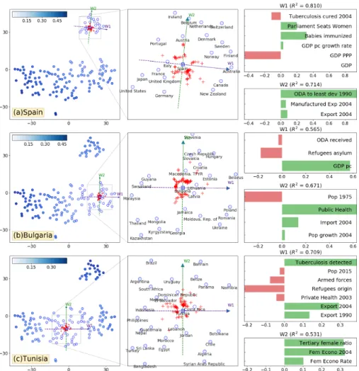
The proposed method is evaluated on the Country dataset [11], which contains 45 socio-economic indicators (e.g. GDP, women in the economy, healthcare, etc.) released in 2007 for 138 countries. The t-SNE visualization is built with a per-plexity of 10. Three countries with very different socio-economic characteris-tics are chosen for the analysis: Spain (Fig. 2a), Bulgaria (Fig. 2b) and Tunisia (Fig. 2c). They are located in different zones of the embedding: Spain at the cen-ter of the occidental cluscen-ter (top-right of the embedding), Bulgaria and Tunisia at the edge and the center of the largest cluster. For each country, the left-most scatter plot represents the original embedding in blue and the projected samples instances in red. The transparency indicates the errors made by the linear model applied on the original instances, which gives an idea of the zone that can be explained. The scatter plot in the middle is a zoom on the region explained. The right-most figure represents the weights to explain the two local dimensions.
The quasi-horizontal trend centered on Spain (W1 in Fig. 2a) is mainly ex-plained by the GDP PPP (purchasing power parity), the healthcare (e.g. babies immunized to measles) and the number of women in the parliament. On this axis, it can be observed that the country at the far right of W1 is Iceland, a small country that is known for having favored the number of women at the parliament. On the other side of the axis, big countries with an effective econ-omy can be found, such as the USA and Japan. The quasi-vertical trend (W2 in Fig. 2a) is uniquely determined by the aid towards developing countries.
The first axis explaining the trend around Bulgaria (W1 in Fig. 2b) is char-acterized by economic and political features. Countries towards the right have higher GDP per capita than Bulgaria ($3109), e.g. Estonia($8331), Croatia ($7724) and Lithuania ($6480), while countries towards the left receive more refugees than Bulgaria (4k), e.g. Guyana (73k) and Malaysia (34k). The second axis (W2 in Fig. 2b) is a mix of demographic, health and economic features. Towards the top, we find countries with larger expenditure on public health and larger imports of good and services than Bulgaria (4.1% and 69% of GDP) like Malta (7.4% and 83%) and Slovakia (5.2% and 79%), while toward the bottom, countries with smaller population in 1975 than Bulgaria (8.7M) can be found,
Fig. 2: Evaluation of the proposed method for explaining the local trends in the t-SNE embedding for three selected countries: Spain, Bulgaria and Tunisia. For each axis, R2measures how well the embedding is linearly and locally explained.
The blue transparency corresponds to the errors of the local model. like Jamaica (2M), Latvia (2.5M) or Moldova (3.8M).
For the local region around Tunisia on the embedding, the horizontal axis (W1 in Fig. 2c) broadly represents countries that have increased exports from 1990 to 2004, have a rather low population, a small armed force and a high rate of tuberculosis detected in 2004. The countries on the right have a greater rate of tuberculosis detected than Tunisia (96%), e.g. Chile (114%), Panama (133%) and Costa Rica (153%). They also export more than Tunisia (45 % of its GDP in 2004), e.g. Panama (63%) and Costa Rica (46%). In contrast, Indonesia on the left has a much lower export rate of only 31%. The vertical axis (W2 in Fig. 2c) represents the place of women in the economy measured by the ratio of male/female enrolled in the tertiary education, the female economic activity rate
in 2004 and the evolution of the female economic activity rate from 1990 to 2004. Considering the rate of female activity in 2004 and the evolution from 1990 to 2004, in the embedding below Tunisia (with 27.9% and 37%), we see Morocco (26.7% and 33%) and Egypt (20.1% and 28%). Above it, we see Dominican Republic (45.5% and 55%) and Uruguay (55.7% and 71%).
It should be noted that some local regions cannot be explained linearly. For instance, BIR does not found any solution for local regions around Denmark and Lithuania. This can be due to the fact that (i) t-SNE makes mistakes in its projection (i.e. it does not make sense to explain it) and (ii) the mapping can be highly non-linear, so much that it is impossible to explain the region linearly.
6
Conclusion
The main contribution of this paper is to adapt LIME, a method designed to explain any predictive model, in order to explain t-SNE embeddings. First, an oversampling method based on SMOTE is used to generate m relevant samples in HD for a selected instance of interest. Second, only the positions of these m newly created samples are computed by t-SNE. Third, a sparse linear model is used to explain the local orthogonal trends around the selected instance. In future works, the proposed approach will be extended to explain embeddings of image and text datasets. The complexity O((m + n)2) of the out-of-sample
projection can also be improved, e.g. with interpolation [12]. Work can also be done to show where local models are relevant in the visualization.
References
[1] L. van der Maaten and G. Hinton. Visualizing data using t-SNE. JMLR, 9(Nov):2579– 2605, 2008.
[2] M. Wattenberg et al. How to use t-SNE effectively. Distill, 1(10):e2, 2016.
[3] M. T. Ribeiro, S. Singh, and C. Guestrin. Why should I trust you?: Explaining the predictions of any classifier. In Proc. of SIGKDD, pages 1135–1144, 2016.
[4] A. Gisbrecht, B. Mokbel, and B. Hammer. Linear basis-function t-SNE for fast nonlinear dimensionality reduction. In Proc. of IJCNN, pages 1–8, 2012.
[5] A. Gisbrecht, A. Schulz, and B. Hammer. Parametric nonlinear dimensionality reduction using kernel t-SNE. Neurocomputing, 147:71–82, 2015.
[6] K. Bunte, M. Biehl, and B. Hammer. A general framework for dimensionality-reducing data visualization mapping. Neural Computation, 24(3):771–804, 2012.
[7] N. V. Chawla, K. W. Bowyer, L. O. Hall, and W. P. Kegelmeyer. SMOTE: synthetic minority over-sampling technique. JAIR, 16:321–357, 2002.
[8] L. Van Der Maaten. Learning a parametric embedding by preserving local structure. In Proc. of AISTATS, pages 384–391, 2009.
[9] A. Bibal, R. Marion, and B. Fr´enay. Finding the most interpretable MDS rotation for sparse linear models based on external features. In Proc. of ESANN, pages 537–542, 2018. [10] R. Marion, A. Bibal, and B. Fr´enay. BIR: a method for selecting the best interpretable multidimensional scaling rotation using external variables. Neurocomputing, 342:83–96, 2019.
[11] United Nations Development Program. Human development report, 2006.
[12] Z. Yang, J. Peltonen, and S. Kaski. Scalable optimization of neighbor embedding for visualization. In Proc. of ICML, pages 127–135, 2013.