Unanimity rule on networks

RESEARCH OUTPUTS / RÉSULTATS DE RECHERCHE

Author(s) - Auteur(s) :

Publication date - Date de publication :

Permanent link - Permalien :

Rights / License - Licence de droit d’auteur :

Bibliothèque Universitaire Moretus Plantin

Institutional Repository - Research Portal

Dépôt Institutionnel - Portail de la Recherche

researchportal.unamur.be

University of Namur

Unanimity rule on networks

Lambiotte, R.; Thurner, S.; Hanel, R.

Physical Review E - Statistical, Nonlinear, and Soft Matter Physics DOI:

10.1103/PhysRevE.76.046101 Publication date:

2007

Document Version

Publisher's PDF, also known as Version of record Link to publication

Citation for pulished version (HARVARD):

Lambiotte, R, Thurner, S & Hanel, R 2007, 'Unanimity rule on networks', Physical Review E - Statistical, Nonlinear, and Soft Matter Physics, vol. 76, no. 4. https://doi.org/10.1103/PhysRevE.76.046101

General rights

Copyright and moral rights for the publications made accessible in the public portal are retained by the authors and/or other copyright owners and it is a condition of accessing publications that users recognise and abide by the legal requirements associated with these rights. • Users may download and print one copy of any publication from the public portal for the purpose of private study or research. • You may not further distribute the material or use it for any profit-making activity or commercial gain

• You may freely distribute the URL identifying the publication in the public portal ? Take down policy

If you believe that this document breaches copyright please contact us providing details, and we will remove access to the work immediately and investigate your claim.

Unanimity rule on networks

Renaud Lambiotte,1 Stefan Thurner,2,3and Rudolf Hanel2

1_{GRAPES, Université de Liège, Sart-Tilman, B-4000 Liège, Belgium} 2

Complex Systems Research Group, HNO, Medical University of Vienna, Währinger Gürtel 18-20, A-1090, Austria 3

Santa Fe Institute, 1399 Hyde Park Road, Santa Fe, New Mexico 87501, USA

共Received 13 March 2007; revised manuscript received 8 June 2007; published 2 October 2007兲

We present a model for innovation, evolution, and opinion dynamics whose spreading is dictated by a unanimity rule. The underlying structure is a directed network, the state of a node is either activated or inactivated. An inactivated node will change only if all of its incoming links come from nodes that are activated, while an activated node will remain activated forever. It is shown that a transition takes place depending on the initial condition of the problem. In particular, a critical number of initially activated nodes is necessary for the whole system to get activated in the long-time limit. The influence of the degree distribution of the nodes is naturally taken into account. For simple network topologies we solve the model analytically; the cases of random and small world are studied in detail. Applications for food-chain dynamics and viral mar-keting are discussed.

DOI:10.1103/PhysRevE.76.046101 PACS number共s兲: 87.23.Ge, 89.65.Ef, 89.75.Fb

I. INTRODUCTION

In general, a discovery, invention, or the emergence of something new depends on the combination of several pa-rameters, all of them having to be simultaneously met. One may think of economy, where the production of a good de-pends on the production or existence of other goods, e.g., to produce a car one needs the wheel, the motor, and some fioritura. In return, this new discovery opens new possibili-ties and needs that will lead to the production of yet new goods, e.g., the simultaneous existence of the car and of al-cohol directly leads to the invention of the air bag, etc. This feedback is responsible for the potential explosion of the number of items, such as observed, e.g., in the Cambrian explosion, and may even lead to a pandemics where all pos-sible items are produced关1兴.

Such autocatalytic processes are very general 关1–4兴 and

obviously apply to many situations not only related to inno-vation, but also to evolution, opinion formation, food chains, etc. Typical examples are the dynamics of scientific ideas, music genres, or any other field where the emergence of a new element possibly leads to new combinations and new elements. In the case of social systems, where it is well known that the activation of an agent may require simulta-neous exposure to multiple active neighbors关5,6兴, one may

think of the spreading of information or rumors between so-cial agents who propagate information only after verifying its validity among several sources, as well as other collective phenomena such as riots, stock market herds, etc.

After mapping the above catalytic reactions onto a net-work structure, where nodes represent items共agents兲 and di-rected links show which items are necessary for the produc-tion of others共which agents influence others兲, it is tempting to introduce a unanimity rule共UR兲: a node on the network is activated only if all the nodes arriving to it through a link are activated. Surprisingly, the dynamics of such an unanimity rule, that is a straightforward generalization of the majority rule of opinion dynamics关7–11兴 and reminds on features of

the voter model关12–16兴, the Axelrod model 关17,18兴 as well

as of Boolean networks关3,19兴, is poorly known 关1兴. Let us

emphasize that UR differs from these previous models by the fact that it is irreversible, i.e., once a node has reached the activated state, it remains in it. From a practical point of view, the irreversible nature of UR makes it an excellent candidate for modeling the adoption of a new technology, e.g., multimedia messaging service共MMS兲 关20兴, by

interact-ing customers. Indeed, technological standards are them-selves irreversible once they are adopted by a population, e.g., a mainstream revival of vinyl records instead of CD’s and MP3’s is more than unlikely. Another specificity of UR is the fact that it is purely deterministic, i.e., once the topol-ogy is fixed and an initial number of nodes are activated, the whole dynamics is determined by the interaction between neighbors. In contrast, the Voter model, when it is applied to a complex network, incorporates a random step when a node chooses among its neighbors with whom it will interact. Similarly, in the majority rule, a node choses randomly two nodes among its neighbors in order to form a majority triplet. We will show below that such random effects alter the spreading on the network and may lead to qualitatively very different features.

The unanimity rule may also be viewed as a limiting case of a threshold model 共TM兲 for decision making scenarios 关21–23兴, except that TM is usually applied to an undirected

network while UR is defined on a directed network. In such a model, a node changes its state if a fraction T, 0ⱕTⱕ1, of its neighbors are in the other state. However, contrary to previous studies, we are not interested in the probability that a cascade is triggered by a single node共or small set of nodes兲 nor in the expected size of the global cascade once it is triggered, but in the evolution of the system when a finite fraction of the nodes is initially activated. In the following, we will therefore look at the relation between the initial number of activated nodes and the final number of activated nodes in the network, and at the condition for a pandemics, i.e., a complete activation of the network, to take place.

The remainder of the paper is organized as follows. In Sec. II, the unanimity rule is introduced. In Sec. III, we de-rive equations for the time evolution of the proportion of

activated nodes. These equations are shown to be nonlocal in time, i.e., they depend explicitly on the initial conditions. They depend on the network topology and exhibit a transi-tion depending on the initial conditransi-tions, i.e., one needs to activate initially a minimum number of nodes to ensure that the whole system gets activated in the long-time limit. We also focus on a simplified topology where each node has exactly two incoming links and re-formalize our description in order to highlight the role played by the local correlations. To do so, we look at all the configurations of nodes and their direct neighbors and show that the system asymptotically reaches a frozen state. In Sec. IV, we successfully compare our predictions with simulations of UR on various topolo-gies. In Sec. V we conclude and make some remarks on practical applications and generalizations of UR.

II. UNANIMITY RULE

Let us now introduce the model in detail. The network is composed of N nodes related through directed links. Each node exists in one of two states: activated or inactivated. The number of nodes with indegree i 共the indegree of a node is defined to be the number of links pointing to it兲 is denoted by

Ni and depends on the underlying network structure. It is

therefore a fixed quantity that does not evolve with time. Initially 共at t=0兲 there are A共0兲 nodes which are activated, among which Ai共0兲 have an indegree i. In general, the total

number of activated nodes at time t is denoted by A共t兲 and the number of nodes of type i, activated at time t, is Ai共t兲.

These quantities satisfy the relation

A共t兲 =

兺

i

Ai共t兲. 共1兲

It is also useful to introduce the quantities ni= Ni/ N and

ai共t兲=Ai共t兲/Niwhich are the proportions of nodes with

inde-gree i in the network 共indegree distribution兲 and the prob-ability that such a node i is activated, respectively. Let us also define

a共t兲 =A共t兲

N =

兺

niai共t兲 共2兲

that is the fraction of activated nodes in the whole network at time t.

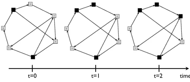
The unanimity rule is defined as follows共see Fig.1兲. At

each time step, each node is considered, i.e., the dynamics is synchronous关24兴. If all the links arriving to an inactivated

node i originate at nodes which are activated at t − 1, i gets activated at t. Otherwise, it remains inactivated. The process is applied iteratively until the system reaches a stationary frozen state, characterized by an asymptotic value aFIN

⬅a共⬁兲. In the following, we are interested in the relation between a_FINand a_IN⬅a共0兲, i.e., what is the final occupation of the network as a function of its initial occupation on a specific network. Let us mention that each node may be pro-duced by only one combination of 共potentially many, de-pending on the indegree兲 nodes. This is a modification of the model of Hanel et al.关1兴, where more than one pairs of 共two兲

nodes could produce new elements and will lead to a differ-ent equation for the activation evolution, as shown below. The dynamics studied here implies that nodes with a higher indegree will be activated with a probability smaller than those with a smaller indegree—because the former have more conditions to be fulfilled.

III. ANALYTICAL APPROACH A. Equation of evolution

Let us now derive an equation of evolution for Ai共t兲 and

A共t兲. To do so it is helpful to consider the first time step and

then to iterate. There are initially A共0兲 activated nodes,

t=0

t=1

t=2

time

FIG. 1. First two steps of UR starting from an initial network of seven nodes, two of them being activated. Initially there is only one node among the nonactivated nodes that satisfies the unanimity rule. It gets therefore activated at the first time step. At that time, there is a new node whose two incoming links come from activated nodes. It gets activated at the second time step. It is straightforward to show that this system gets fully activated at the fourth time step.

LAMBIOTTE, THURNER, AND HANEL PHYSICAL REVIEW E 76, 046101共2007兲

Ai共0兲=A共0兲Ni/ N of them being of indegree i on average共the

activated nodes are randomly chosen in the beginning兲. The ensemble of Ai共0兲 nodes is called the initial set of indegree i.

By construction, the probability that i randomly chosen nodes are initially activated, is ai共0兲 共i is an exponent兲. The average number of nodes with indegree i and which respect the unanimity rule is therefore Niai共0兲. Among these nodes,

Nia共0兲ai共0兲 were already activated initially. This is due to the

fact that the total number of nodes with degree i that are initially activated is Nia共0兲. Consequently, the number of

nodes that gets activated at the first time step is

⌬i共0兲 = 关Ni− Nia共0兲兴ai共0兲 共3兲

and, on average, the total number of occupied nodes with indegree i evolves as

Ai共1兲 = Ai共0兲 + ⌬i共0兲. 共4兲

At the next time step, the average number of nodes with indegree i, which respect the unanimity rule and which are outside the initial set is 关Ni− Nia共0兲兴ai共1兲. Among those

nodes,⌬i共0兲 have already been activated during the first time

step, so that the average number of nodes which get activated at the second time step is

⌬i共1兲 = 关Ni− Nia共0兲兴关ai共1兲 − ai共0兲兴. 共5兲

Note that Eq. 共5兲 is valid because no node in ⌬i共1兲 also

belongs to⌬i共0兲. This is due to the fact that each node can

only be activated by one combination of i nodes in our model, so that no redundancy is possible between⌬i共1兲 and

⌬i共0兲. By proceeding similarly, it is straightforward to show

that the contributions⌬i共t兲 read

⌬i共t兲 = 关Ni− Nia共0兲兴关ai共t兲 − ai共t − 1兲兴, 共6兲

with a共−1兲=0, by convention. The number of activated nodes evolve as

Ai共t + 1兲 = Ai共t兲 + ⌬i共t兲. 共7兲

By dividing Eq.共7兲 by Ni, one gets a set of equations for the

proportion of nodes ai苸关0,1兴:

ai共t + 1兲 = ai共t兲 + 关1 − a共0兲兴关ai共t兲 − ai共t − 1兲兴, 共8兲

where the coupling between the different proportions ai共t兲

occurs through the average value a共t兲=兺iniai共t兲, as defined

above. Finally, by multiplying Eq.共8兲 by the indegree

distri-bution niand summing over all values of i, one gets a closed

equation for the average proportion of activated nodes in the network that reads

a共t + 1兲 = a共t兲 + 关1 − a共0兲兴

兺

i

ni关ai共t兲 − ai共t − 1兲兴. 共9兲

Let us stress that Eq. 共9兲 is nonlinear as soon as ni⫽0, i

⬎1. Moreover, it is characterized by the nontrivial presence of the initial condition a共0兲 in the right-hand side nonlinear term and is therefore nonlocal in time. One should stress that this nonlocality is a feature of the effective mean field de-scription and not of the UR itself, where, by construction, the configuration of the system at time t + 1 is fully determined

by its configuration at time t. The origin for this nonlocality in the mean field description will be discussed further in Sec. III C. Finally, let us also note that Eq. 共9兲 explicitly shows

how the indegree distribution ni affects the propagation of

activated nodes in the system.

B. Some special cases

Let us now focus on simple choices of ni in order to

apprehend analytically the behavior of Eq.共9兲. The simplest

case is ni=␦i1 共each node has one incoming link兲 for which

Eq.共9兲 reads

a共t + 1兲 = a共t兲 + 关1 − a共0兲兴关a共t兲 − a共t − 1兲兴. 共10兲

This equation is solved by recurrence:

a共1兲 = a共0兲 + 关1 − a共0兲兴a共0兲, a共2兲 = a共0兲 + 关1 − a共0兲兴a共0兲

+关1 − a共0兲兴兵a共0兲 + 关1 − a共0兲兴a共0兲 − a共0兲其

=a共0兲 + 关1 − a共0兲兴a共0兲 + 关1 − a共0兲兴2_{a共0兲 共11兲}

and, in general, a共t兲 =

兺

a共t + 1兲 =

兺

冉

兺

兺

冊

兺

The above solution implies that any initial condition a共0兲 ⫽0 converges toward the asymptotic state aFIN= 1, i.e.,

whatever the initial condition, the system is fully activated in the long time limit. From Eq.共12兲, one finds that the

relax-ation to a_FIN= 1 is exponentially fast, a共t兲⬇1−et ln关1−a共0兲兴_.

Let us now focus on the more challenging case ni=␦i2

where all the nodes have an indegree of 2 by construction. In that case, Eq.共9兲 reads

a共t + 1兲 = a共t兲 + 关1 − a共0兲兴关a2共t兲 − a2共t − 1兲兴. 共14兲

The nonlinear term does not allow one to find a simple re-currence expression as above. However, numerical integra-tion of Eq.共14兲 shows that the leading terms in the Taylor

expansion of a共t兲 behave as

a共t兲 =

兺

i=1 t+1

ai共0兲 + O共t + 2兲, 共15兲

a共⬁兲 = a共0兲

1 − a共0兲. 共16兲 This solution should satisfy the normalization constraint

a共⬁兲ⱕ1, so that it can hold only for initial conditions a共0兲

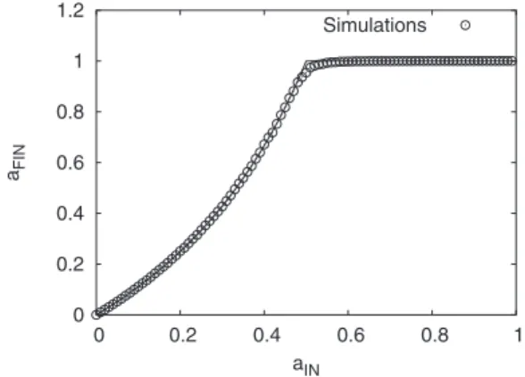
⬍1/2. This argument suggest that a transition takes place at

ac= 1 / 2, such that only a fraction of the whole system gets

activated when a共0兲⬍ac while the whole system activates

above this value 共see Fig. 2兲. We verify the approximate

solution共16兲 by looking for a solution of the form

a共t兲 = a共0兲

1 − a共0兲关1 +⑀共t兲兴. 共17兲 By inserting this expression into Eq.共14兲, one gets the

recur-rence relations

⑀共t + 1兲 =⑀共t兲 + a共0兲关1 +⑀共t兲兴2_{− a共0兲关1 +⑀共t − 1兲兴}2_,

⑀共t + 1兲 =⑀共t兲 + 2a共0兲关⑀共t兲 −⑀共t − 1兲兴, 共18兲 where the second line is obtained by keeping only first order corrections in⑀. In the continuous time limit, keeping terms until the second time derivative, one obtains

关1 − 2a共0兲兴⳵t⑀共t兲 + 1/2关1 + 2a共0兲兴⳵t

2_{⑀共t兲 = 0, 共19兲}

whose exponential solutions read⑀共t兲=e−␭twith ␭ =1

2

关1 − 2a共0兲兴

关1 + 2a共0兲兴. 共20兲 This is a relaxation to the stationary state a共⬁兲, only when

a共0兲⬍1/2, thereby confirming a qualitative change at ac

= 1 / 2. Contrary to the case␦_i1, there is therefore a transition, reminding the behavior observed in Refs.关1,22兴 and the

ex-istence of critical mass, i.e., a critical value ac= 1 / 2 under

which only a fraction of the whole system is asymptotically activated.

Before going further, it is interesting to focus on a variant of UR in order to highlight the importance of its determinis-tic nature. This variant is defined as follows. Let us consider a directed network where nodes have on average a high in-degree. For the sake of simplicity, we consider a fully con-nected network, i.e., each node receives a link from all the

N − 1 other nodes. At each time step, all the nodes randomly

select two of their neighbors, in a way that reminds on the process of Eq.共14兲 and it gets activated only if both

neigh-bors were activated at the previous time step. It is straight-forward to show that the equation of evolution for atis now

a共t + 1兲 = a共t兲 + 关1 − a共t兲兴a2共t兲 共21兲

and that aFIN= 1, i.e., all the nodes are asymptotically

acti-vated, whatever the initial condition aIN, except if aIN= 0.

The difference from the relation Eq.共16兲 of UR is due to the

fact that the inclusion of random effects mixes the different configurations of the system, i.e., in a mean field way, and therefore multiplies the possibility for nodes to be activated.

C. Alternative description: The role of correlations

Let us now return to UR and emphasize some points that deserve attention. First, one should note that the critical pa-rameter of the above transition is not an external papa-rameter, but it is the initial condition aINitself, i.e.,

aFIN

再

=1 if a_IN⬎ ac,

⬍1 otherwise. 共22兲 Such a dependence on initial conditions has also been ob-served in Axerod dynamics关25–27兴 or minority games 关28兴.

Equation 共22兲 also implies that UR has a continuum of

at-tractors, i.e., the asymptotic state of the systems is not lim-ited to a few fixed points, each of them surrounded by its own basin of attraction, but the whole range of values a 苸关0,1兴 may be a stationary solution depending on the initial condition aIN 关this can be seen from Fig. 2 as the curve aFIN共aIN兲 goes continuously from 0 to 1兴. Finally, one should

also stress that the nonlocality in time of the dynamical equa-tions Eq. 共9兲 implies that the same value a共t兲 will reach a

different stationary state aFIN depending on the time t at

which it is attained.

In order to understand the origin of these peculiar proper-ties, it is useful to tackle the problem analytically from a different point of view. To do so, let us focus on networks where all the nodes have an indegree of 2, i.e., ni=␦i2. The

state of a node may either be A for activated or I for inacti-vated, but, in order to calculate its state at the next step, one also needs to know the state of its two neighbors. Conse-quently, we represent the state of a node by a triangle 共see Fig.3兲 composed of this node and of its two incoming

neigh-bors. Let N_␣

0;␣1␣2 be the number of such triangular

configu-rations where a node in state␣₀receives its first link from a node in state␣1and a second link from a node in state␣2.␣i

may be A共activated兲 or I 共inactivated兲. The equations of evolution for N_␣

0;␣1␣2are easily found to

be共see Fig.3兲 0 0.2 0.4 0.6 0.8 1 1.2 0 0.2 0.4 0.6 0.8 1 aFIN aIN Simulations

FIG. 2. Relation a_FIN共a_IN兲 obtained by integrating numerically Eq.共14兲 共solid line兲 and by performing simulations of the model on

a network with n_i=␦_i2. The system obviously shows a transition at

a共0兲=1/2. Moreover, the prediction, Eq. 共16兲 is in perfect

agree-ment共indistinguishable from the solid line兲 with the numerical in-tegration of Eq. 共14兲. The simulations were performed with N

= 10 000 nodes and the results are averaged over 100 realizations of the process.

LAMBIOTTE, THURNER, AND HANEL PHYSICAL REVIEW E 76, 046101共2007兲

NA;AA共t + 1兲 = NA;AA共t兲 + NI;AA共t兲 +␲I→ANA;AI共t兲 +␲I→A 2 NA;II共t兲, NA;II共t + 1兲 =␲I→I 2 NA;II共t兲,

NA;AI共t + 1兲 =␲I_→INA;AI共t兲 + 2␲I_→A␲I_→INA;II共t兲,

N_I;II共t + 1兲 =␲I2_→INI;II共t兲,

NI;AA共t + 1兲 =␲I2→ANI;II共t兲 +␲I_→ANI;AI共t兲,

N_I;AI共t + 1兲 =␲I→INI;AI共t兲 + 2␲I→A␲I→INI;II共t兲, 共23兲

where we have taken into account the fact that an inactivated node whose two incoming neighbors are activated will be activated at the next time step and that an activated node remains activated forever. The quantities␲I_→Aand␲I_→Aare

the probabilities for an inactivated incoming neighbor to get activated and to remain inactivated, respectively. These quantities obviously respect

␲I_→I= 1 −␲I_→A. 共24兲

In order to close the system of equations 共23兲, we evaluate

the transition probability ␲I_→Aby the probability for a

ran-domly selected node I to have two activated incoming neigh-bors

␲I→A=

NI;AA

NI;AA+ NI;AI+ NI;II

. 共25兲 Let us also introduce the total number of activated nodes

NA=兺␣₁,␣₂NA;␣₁␣₂ 关which is equal to A of Eq. 共1兲兴 and the

total number of inactivated nodes NI=兺␣₁,␣₂NI;␣₁␣₂. By

sum-ming over the states of the incosum-ming neighbors, one also finds

NA共t + 1兲 = NA共t兲 + NI;AA共t兲,

NI共t + 1兲 = NI共t兲 − NI;AA共t兲, 共26兲

which confirms that only the configurations NI;AA drive the

evolution of the system and that a stationary state is reached

when NI;AA= 0. This also shows that the stationary state is

frozen, as no change is possible when N_I;AA= 0. In some sense, the number of dynamic triangles NI;AAmay therefore

be viewed as the potential of the network to change, and the evolution stops, whatever its state, when all the dynamic triangles have been transformed into other triangles.

Let us now focus on the initial conditions of the system of equations共23兲. In principle, many initial conditions may be

chosen, each of them leading to a different trajectory in the six-dimensional dynamical space. However, initial condi-tions are subject to several constraints. On the one hand, the following equality has to hold:

兺

␣0,␣1,␣2 N_␣

0;␣1␣2= N, 共27兲

which is just a normalization, but initial conditions must also satisfy the conservation law

TA= 2NA,

TI= 2NI, 共28兲

where the quantities

TA= 2NA;AA+ 2NI;AA+ NA;AI+ NA;AI,

TI= 2NA;II+ 2NI;II+ NA;AI+ NA;AI 共29兲

are the total number of activated 共inactivated兲 incoming neighbors in triangles. Relation 共28兲 therefore means that

each node that is an incoming neighbor in a triangle is also at the summit of another triangle共as it also receives two incom-ing links by construction兲. It is important to stress that the constraints共28兲 are preserved by the dynamics 共23兲. Indeed,

one verifies easily that

TA共t + 1兲 − 2NA共t + 1兲 =␲I→I关TA共t兲 − 2NA共t兲兴,

TI共t + 1兲 − 2NI共t + 1兲 =␲I→I关TI共t兲 − 2NI共t兲兴 共30兲

so that Eq.共28兲 holds all times if it holds at t=0.

One should emphasize that there are many configurations

N_␣

0;␣1␣2 of the six-dimensional space that satisfy the

con-straints共27兲 and 共28兲 and that have the same average number

of activated nodes NA. However, the NA= Na0nodes that are

initially activated are randomly chosen. Consequently, there are no correlations between the states of neighboring nodes and, among all the possible configurations for which NA

= Na₀, the initial condition is actually

NA;AA共0兲 = Na3共0兲,

N_A;II共0兲 = Na共0兲关1 − a共0兲兴2_, NA;AI共0兲 = 2Na2共0兲关1 − a共0兲兴,

NI;II共0兲 = N关1 − a共0兲兴3,

N_I;AA共0兲 = N关1 − a共0兲兴a2共0兲,

FIG. 3. Transition probabilities between the six possible trian-gular configurations. The dynamics is obviously irreversible, with a preferred direction toward the activated共black兲 state.

NI;AI共0兲 = 2N关1 − a共0兲兴2a共0兲. 共31兲

One verifies easily that Eq.共31兲 respects the constraints 共27兲

and共28兲.

A recursive integration of the system of Eqs.共23兲 starting

from the initial conditions共31兲 has been performed by using

MATHEMATICA. It is found that the resulting a共t兲 is identical

to that obtained by integrating Eq. 共14兲 starting from the

same initial condition a共0兲, so that the relation aFIN共aIN兲 is

also identical. However, an analytical demonstration of the equivalence of Eqs. 共23兲 and 共14兲 is still lacking—we are

open to suggestions.

Looking at Eqs. 共23兲 and 共14兲 as two sides of the same

process, one may now understand why the same value of a共t兲 may lead to different stationary solutions aFIN. Indeed, it is

easy to show that the system of Eqs.共23兲 develops

correla-tions in the course of time, i.e., in general, the configuracorrela-tions

N_␣

0;␣1␣2共t兲 cease to fulfill the following relations when t⬎0: NA;AA共t兲 = Na3共t兲,

N_A;II共t兲 = Na共t兲关1 − a共t兲兴2_, NA;AI共t兲 = 2Na2共t兲关1 − a共t兲兴,

NI;II共t兲 = N关1 − a共t兲兴3,

NI;AA共t兲 = N关1 − a共t兲兴a2共t兲,

NI;AI共t兲 = 2N关1 − a共t兲兴2a共t兲, 共32兲

where a共t兲=NA/ N. This result is obvious for t→⬁ and 0

⬍aIN⬍ac, as we have shown that 0⬍a共⬁兲⬍1, while NI,AA

= 0 in that case. The emergence of such correlations implies that the same value of a共t兲, for different values of t, may correspond to different configurations N_␣

0;␣1␣2 and may

therefore lead to a different trajectory in the six-dimensional space. Consequently, a different asymptotic state aFINmay be

reached in principle.

Before going further, one should note that a generalization of Eqs.共23兲 for more general degree distributions niis not an

easy task, as it implies a multiplication of the number of variables to take into account. The formalism 共9兲 is to be

preferred in that case.

IV. SIMULATIONS

Let us now verify the above predictions by performing numerical simulations of the model. To do so, one has first to build networks whose indegrees are␦iK, i.e., the indegree of

each node is exactly K, where K = 1 for Eq.共12兲 and K=2 for

Eq.共16兲. Such networks are easily implemented by picking

randomly K nodes l1, l2, . . . , lK for each node i苸关1,N兴 and

adding links going from l1, l2, . . . , lKto i. Once the

underly-ing network is built, we randomly assign a共0兲N activated nodes to the network and apply the unanimity rule until a stationary state is reached. The asymptotic value aFIN

⬅a共⬁兲 is averaged over several realizations of the process 共on several realizations of the underlying network兲 and is

shown to be in excellent agreement with the theoretical pre-dictions. The case K = 2 is plotted in Fig.2, but other values of K have also been studied and suggest that ac共K兲=1

− 1 / K. This behavior is expected as nodes with a higher de-gree require more conditions for an activation, so that the asymptotic number of activated nodes is reduced.

We have also focused on more realistic topologies and compared the results obtained from Eq.共9兲 with numerical

simulations of the UR. Two types of networks are discussed in the following, purely random networks 关29兴 and

small-world-like networks 关30兴, but other types have also been

considered and lead to the same conclusions. The random network was obtained by randomly assigning L directed links over N nodes, so that its degree distribution is

nk= e−␭

␭k

k!, 共33兲

where ␭=L/N. The small-world network was obtained by starting from a directed ring configuration and then randomly assigning L directed links共shortcuts兲 over the nodes, i.e., the total number of links in that case is L + N 共The network drawn in Fig.1 is such network with N = 7 nodes and L = 3 short cuts兲. In that case, the degree distribution is easily found to be nk=

冦

Let us note that the directed small-world network can be viewed as a food chain with a well-defined hierarchy be-tween species together with some random short cuts. In that case, UR can be interpreted as an extinction model: if all the species that one particular species can eat, go extinct, this species will also die out.

To compare the simulation results with the theoretical pre-dictions, we integrate Eq.共9兲 with the corresponding degree

distributions of Eqs.共33兲 and 共34兲. The agreement is

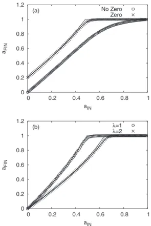
excel-lent, except close to the transition points where finite size effects are expected. One observes关Fig.4共b兲兴 by increasing the average degree that the location of the transition ac is

closer and closer to 1, for the same reason such a shift took place in the case of␦iKnetworks.

One should also stress that each node receives at least one incoming link by construction共n0= 0兲 in␦iKnetworks and in

small-world network. This is not the case for random net-works关see Eq. 共33兲兴, for which one has to discuss the

am-biguous dynamics of nodes with zero incoming links. Two choices are possible. Either these nodes cannot be activated in the course of time, because they are not reached by any other node共no-zero version兲, or all of them get activated at the first time step, thereby assuming that their activation does not require any first knowledge共Zero version兲. The choice is a question of interpretation. The two versions are associated to different evolution equations, namely,

LAMBIOTTE, THURNER, AND HANEL PHYSICAL REVIEW E 76, 046101共2007兲

a共t + 1兲 = a共t兲 + 关1 − a共0兲兴

兺

i=1

⬁

ni关ai共t兲 − ai共t − 1兲兴 共35兲

for the no-zero version, and

a共t + 1兲 = a共t兲 + 关1 − a共0兲兴

兺

i=0

⬁

ni关ai共t兲 − ai共t − 1兲兴 共36兲

for the zero version. When n₀= 0, the above equations are obviously equivalent. The two interpretations lead to quite different behaviors关Fig.4共a兲兴. As expected, there are always more activated nodes in the zero version than in the no-zero version. This effect even provokes qualitative differences be-tween the versions, i.e., as shown in Fig. 4共a兲, there is no critical value acfor the no-zero version while ac⬇0.48 for

the zero version.

Before concluding, let us stress that the difference be-tween the two interpretations is more pronounced when the number of nodes with zero incoming links becomes higher. This is the case for growing networks, e.g., the Barabási-Albert network关31兴, that are well-known models for

scale-free networks. We have verified this effect by studying nu-merically UR on a network that was built starting from one

seed node and adding nodes one at a time until the system is composed of N nodes关32兴. At each step, the node first

con-nects to a randomly chosen node and, with probability r, it redirects its link to the father of the selected node. This method is well known to be equivalent to preferential attach-ment and to lead to the formation of fat-tail degree distribu-tions k−␯, with␯= 1 + 1 / r关32,33兴, while the number of nodes

with zero incoming links is very large. We have studied sev-eral values of␯close to␯= 3 and it is shown共see Fig.5兲 that

all the nodes are finally activated whatever the initial condi-tion in the zero version共ac= 0兲, while there is no transition in

the no zero version共ac= 1兲. It is also interesting to point that

an integration of the Eqs.共35兲 and 共36兲 reproduce the same

extreme behavior.

V. CONCLUSION

To summarize, we have introduced a simple model for innovation whose dynamics is based on the unanimity rule. It is shown that the discovery of new items on the underlying network opens perspectives for the discovery of yet new items. This feedback effect may lead to complex spreading properties, embodied by the existence of a critical size for the initial activation, that is necessary for the complete acti-vation of the network in the long-time limit. The problem has been analyzed numerically on a large variety of network structures and has been successfully described by recurrence relations for the average activation. Let us stress that these recurrence relations have a quite atypical form due to their explicit dependence on initial conditions. Moreover, their nonlinearity makes them a hard problem to solve in general. We have also shown that the system might be studied alter-natively by focusing on the configurations of nodes and their direct neighbors, thereby highlighting the role of internal correlations and clarifying the origin of the nonlocality in time of the recurrence relations.

0 0.2 0.4 0.6 0.8 1 1.2 0 0.2 0.4 0.6 0.8 1 aFIN aIN

(a) No Zero_Zero

0 0.2 0.4 0.6 0.8 1 1.2 0 0.2 0.4 0.6 0.8 1 aFIN aIN (b) λ=1 λ=2

FIG. 4. 共a兲 Relation a_FIN共a_IN兲 obtained for random networks with L = 2N. The no zero and zero versions共see text兲 are shown. 共b兲

a_FIN共a_IN兲 for small-world networks with L=␭N short-cuts. The

simulations were performed with N = 10 000 nodes and the results are averaged over 100 realizations of the process. The solid lines are the numerical solutions of Eqs.共35兲 and 共36兲 and Eq. 共9兲,

re-spectively, evaluated with the corresponding degree distributions, given in Eqs.共33兲 and 共34兲.

0 0.2 0.4 0.6 0.8 1 1.2 0 0.2 0.4 0.6 0.8 1 aFIN a_IN No Zero Zero

FIG. 5. aFIN共aIN兲 for a network with redirection. The total

num-ber of nodes is N = 10 000, r = 1 / 2 and the results are averaged over 100 realizations. In the zero version, one observes that all the nodes are finally activated whatever the initial condition. In the no zero version, in contrast, the full activation of the network is attained only when aIN= 1. The solid lines correspond to numerical

integra-tions of Eqs. 共35兲 and 共36兲 with the corresponding degree

Finally, let us emphasize that unanimity rule is a general mechanism that should apply to numerous situations related to innovation, opinion dynamics, or even species and popu-lation dynamics. Practically, one may think of the adoption of a new technological standard in a population of interacting customers or the propagation of rumors between social agents, the key ingredient of UR being that many conditions have to be simultaneously met in order to drive the activation of a node. We have shown that UR naturally leads to the notion of critical mass, which might have important conse-quences, in marketing, for instance, as it suggests that an efficient viral marketing campaign关34兴 should reach a

mini-mum number of customers in order to ensure the propagation of the message through the whole network. Moreover, the results of Sec. IV also suggest that a targeted attack关35,36兴,

i.e., a strategic choice of initially activated nodes instead of a random choice, might alter, and possibly accelerate, the spreading of the process. This is due to the fact that many triangle configurations N_␣

0,␣1,␣2correspond to the same value

of a共0兲, each of them corresponding to a different time evo-lution of a共t兲.

Finally, one should also stress that UR is a very extreme dynamics that may lead to counterintuitive features, i.e., the propagation becomes slower as the network gets more con-nected. This effect can be circumvented by softening the unanimity rule, for instance, by requiring that only a finite number of neighbors has to be activated for an activation. We will show elsewhere that this variation—unfortunately more complicated—leads to qualitatively similar results共existence of ac兲 without such unrealistic features.

To conclude, we hope that in the above sense this paper will form part of a set of works 共activated nodes兲 which allow for the activation of novel共yet inactive兲 perspectives and research directions.

ACKNOWLEDGMENTS

This collaboration was made possible by a COST-P10 short term mission. R.L. has been supported by European Commission Project No. CREEN FP6-2003-NEST-Path-012864. S.T. is grateful to Austrian Science Foundation projects Nos. P17621 and P19132. We would like to thank J.P. Boon and P. Klimek for fruitful comments.

关1兴 R. Hanel, S. A. Kauffman and S. Thurner, Phys. Rev. E 72, 036117共2005兲.

关2兴 J. D. Farmer, S. A. Kauffman, and N. H. Packard, Physica D 22, 50共1986兲.

关3兴 S. A. Kauffman, The Origins of Order 共Oxford University Press, London, 1993兲.

关4兴 R. Hanel, S. A. Kauffman, and S. Thurner, Phys. Rev. E 76, 036110共2007兲.

关5兴 M. Granovetter, Am. J. Sociol. 83, 1420 共1978兲. 关6兴 S. E. Asch, Sci. Am. 193, 31 共1955兲.

关7兴 P. L. Krapivsky and S. Redner, Phys. Rev. Lett. 90, 238701 共2003兲.

关8兴 M. Mobilia and S. Redner, Phys. Rev. E 68, 046106 共2003兲. 关9兴 R. Lambiotte, M. Ausloos, and J. A. Hołyst, Phys. Rev. E 75,

030101共R兲 共2007兲.

关10兴 R. Lambiotte, Europhys. Lett. 78, 68002 共2007兲.

关11兴 R. Lambiotte and M. Ausloos, J. Stat. Mech.: Theory Exp. 共2007兲, P08026.

关12兴 E. Ben-Naim, L. Frachebourg, and P. L. Krapivsky, Phys. Rev. E 53, 3078共1996兲.

关13兴 V. Sood and S. Redner, Phys. Rev. Lett. 94, 178701 共2005兲. 关14兴 C. Castellano, D. Vilone, and A. Vespignani, Europhys. Lett.

63, 153共2003兲.

关15兴 C. Castellano, V. Loreto, A. Barrat, F. Cecconi, and D. Parisi, Phys. Rev. E 71, 066107共2005兲.

关16兴 K. Suchecki, V. M. Eguíluz, and M. S. Miguel, Phys. Rev. E 72, 036132共2005兲.

关17兴 R. Axelrod, J. Conflict Resolut. 41, 203 共1997兲. 关18兴 D. Stauffer, AIP Conf. Proc. 779, 56 共2005兲.

关19兴 M. Huxham, S. Beaney, and D. Raffaelli, J. Theor. Biol. 22, 437共1969兲.

关20兴 http://en.wikipedia.org/wiki/Multimedia_Messaging_Service 关21兴 D. J. Watts, Proc. Natl. Acad. Sci. U.S.A. 99, 5766 共2002兲. 关22兴 P. S. Dodds and D. J. Watts, Phys. Rev. Lett. 92, 218701

共2004兲.

关23兴 D. Centola, V. M. Eguíluz, and M. W. Macy, Physica A 374, 449共2007兲.

关24兴 Z. Mihailović and M. Rajković, Physica A 365, 244 共2006兲. 关25兴 C. Castellano, M. Marsili, and A. Vespignani, Phys. Rev. Lett.

85, 3536共2000兲.

关26兴 K. Klemm, V. M. Eguíluz, R. Toral, and M. San Miguel, Physica A 327, 1共2003兲.

关27兴 F. Vazquez and S. Redner, Europhys. Lett. 78, 18002 共2007兲. 关28兴 M. Marsili and D. Challet, Phys. Rev. E 64, 056138 共2001兲. 关29兴 P. Erdős and A. Rényi, Publ. Math. Inst. Hung. Acad. Sci. 5,

17共1960兲.

关30兴 D. J. Watts and S. H. Strogatz, Nature 共London兲 393, 440 共1998兲.

关31兴 A.-L. Barabási and R. Albert, Science 286, 509 共1999兲. 关32兴 P. L. Krapivsky and S. Redner, Phys. Rev. E 63, 066123

共2001兲.

关33兴 R. Lambiotte, J. Stat. Mech.: Theory Exp. 共2007兲, P02020. 关34兴 J. Leskovec, L. A. Adamic, and B. A. Huberman, e-print

arXiv:physics/0509039.

关35兴 R. Pastor-Satorras and A. Vespignani, Phys. Rev. Lett. 86, 3200共2001兲.

关36兴 R. M. May and A. L. Lloyd, Phys. Rev. E 64, 066112 共2001兲. LAMBIOTTE, THURNER, AND HANEL PHYSICAL REVIEW E 76, 046101共2007兲