RESEARCH OUTPUTS / RÉSULTATS DE RECHERCHE
Author(s) - Auteur(s) :
Publication date - Date de publication :
Permanent link - Permalien :
Rights / License - Licence de droit d’auteur :
Bibliothèque Universitaire Moretus Plantin
Emerging structures in social networks guided by opinions' exchanges
Carletti, Timoteo; Fanelli, Duccio; Righi, Simone
Published in:
Advances in Complex Systems
Publication date:
2011
Document Version
Publisher's PDF, also known as Version of record
Link to publication
Citation for pulished version (HARVARD):
Carletti, T, Fanelli, D & Righi, S 2011, 'Emerging structures in social networks guided by opinions' exchanges',
Advances in Complex Systems, vol. 14, no. 1, pp. 13-30.
General rights
Copyright and moral rights for the publications made accessible in the public portal are retained by the authors and/or other copyright owners and it is a condition of accessing publications that users recognise and abide by the legal requirements associated with these rights. • Users may download and print one copy of any publication from the public portal for the purpose of private study or research. • You may not further distribute the material or use it for any profit-making activity or commercial gain
• You may freely distribute the URL identifying the publication in the public portal ?
Take down policy
If you believe that this document breaches copyright please contact us providing details, and we will remove access to the work immediately and investigate your claim.
c
°World Scientific Publishing Company
On the evolution of a social network
TIMOTEO CARLETTI D´epartement de math´ematique
Facult´es Universitaires Notre Dame de la Paix, rempart de la Vierge 8 Namur, B5000, Belgium
[email protected] DUCCIO FANELLI
Dipartimento di Energetica and CSDC Universit`a di Firenze, and INFN via S. Marta, 3, 50139 Firenze, Italy
[email protected] SIMONE RIGHI D´epartement de math´ematique
Facult´es Universitaires Notre Dame de la Paix, rempart de la Vierge 8 Namur, B5000, Belgium
[email protected] Received (received date)
Revised (revised date)
In this paper we show that the small world and weak ties phenomena can spontaneously emerge in a social network of interacting agents. This dynamics is simulated in the frame-work of a simplified model of opinion diffusion in an evolving social netframe-work where agents are made to interact, possibly update their beliefs and modify the social relationships according to the opinion exchange.
Keywords: Opinion dynamics; social network; small world; weak ties.
1. Introduction
Modeling social phenomena represents a major challenge that has in recent years attracted a growing interest. Insight into the problem can be gained by resorting, among others, to the so called Agent Based Models, an approach that is well suited to bridge the gap between hypotheses concerning the microscopic behavior of indi-vidual agents and the emergence of collective phenomena in a population composed of many interacting heterogeneous entities.
Constructing sound models deputed to return a reasonable approximation of the scrutinized dynamics is a delicate operation, given the degree of arbitrariness in assigning the rules that govern mutual interactions. In the vast majority of cases, data are scarce and do not sufficiently constrain the model, hence the provided
answers can be questionable. Despite this intrinsic limitation, it is however impor-tant to inspect the emerging dynamical properties of abstract models, formulated so to incorporate the main distinctive traits of a social interaction scheme. In this paper we aim at discussing one of such models, by combining analytical and nu-merical techniques. In particular, we will focus on characterizing the evolution of the underlying social network in terms of dynamical indicators.
It is nowadays well accepted that several social groups display two main features: the small world property [24] and the presence of weak ties [15]. The first property implies that the network exhibits clear tendency to organize in densely connected clusters. As an example, the probability that two friends of mine are also, and inde-pendently, friends to each other is large. Moreover, the shortest path between two generic individuals is small as compared to the analogous distance computed for a random network made of the same number of individuals and inter-links connec-tions. This observation signals the existence of short cuts in the social tissue. The second property is related to the cohesion of the group which is mediated by small groups of well tied elements, that are conversely weakly connected to other groups. The skeleton of a social community is hence a hierarchy of subgroups.
A natural question arise on the ubiquity of the aforementioned peculiar aspects, distinctive traits of a real social networks: can they eventually emerge, starting from a finite group of initially randomly connected actors? We here provide an answer to this question in the framework of a minimalistic opinion dynamics model, which exploit an underlying substrate where opinions can flow. More specifically, the network that defines the topological structure is imagined to evolve, coupled to the opinions and following a specific set of rules: once two agents reach a compromise and share a common opinion, they also increase their mutual degree of acquaintance, so strengthing the reciprocal link. In this respect, the model that we are shortly going to introduce hypothesize a co-evolution of opinions and social structure, in the spirit of a genuine adaptive network [16, 25].
Working within this framework, we will show that an initially generated random group, with respect to both opinion and social ties, can evolve towards a final state where small worlds and weak ties effects are indeed present. The results of this paper constitute the natural follow up of a series of papers [3, 10, 9], where the time evolution of the opinions and affinity, together with the fragmentation vs. polarization phenomena, have been discussed.
Different continuous opinion dynamics models have been presented in literature, see for instance [13, 14, 11], dealing with the general consensus problem. The aim is to shed light onto the assumptions that can eventually yield to fixation, a final mono-clustered configuration where all agents share the same belief, starting from an initial condition where the inspected population is instead fragmented into several groups. In doing so, and in most cases, a fixed network of interactions is a priori imposed [2], and the polarization dynamics studied under the constraint of the imposed topology. At variance, and as previously remarked, we will instead allow the underlying network to dynamically adjust in time, so modifying its initially
imposed characteristics. Let us start by revisiting the main ingredients of the model. A more detailed account can be found in [3].
Consider a closed group of N agents, each one possessing its own opinion on a given subject. We here represent the opinion of element i as a continuous real variable Oi∈ [0, 1]. Each agent is also characterized by its affinity score with respect to the remaining N − 1 agents, namely a vector αij, whose entries are real number defined in the interval [0, 1]: the larger the value of the affinity αij, the more reliable the relation of i with the end node j.
Both opinion and affinity evolve in time because of binary encounters between agents. It is likely that more interactions can potentially occur among individuals that are more affine, as defined by the preceding indicator, or that share a close opinion on a debated subject. Mathematically, these requirements can be accommo-dated for by favoring the encounters between agents that minimizes a social metric , as defined below. More concretely, select at random, with uniform probability, the agent i and quantify its social distance with the other members of the community: this is the N −1 vector dij = |∆Ot
ij|(1−αtij), where ∆Oijt = Oti−Ojtis the opinions’ difference of agents i and j at time t. The smaller the value of dt
ij the closer the agent j to i, both in term of affinity and opinion. Mutual affinity can in fact miti-gate the difference in opinion, thus determining the degree of social similarity of two individuals, an observation that inspires the proposed definition of dtij. A Gaussian random perturbation Nj(0, σ) (mean zero and variance σ) is added to dt
ij so to mimic the impact of a social mixing effect, the obtained vector Dt
ij = dtij+ Nj(0, σ) being the social metric. The second agent j for the paired interaction is the one closer to i with respect to Dt
ij. For a more detailed analysis on the interpretation of σ as a social temperature responsible of a increased mixing ability of the popu-lation, we refer to [3, 10, 9]. Let us observe that other models, see for instance [23, 6, 18], make use of the social temperature concept: beyond the specificity of each the formulation, the social temperature is always invoked to control the degree of mixing in the population.
Once two agents are selected for interaction they possibly update their opinions (if they are affine enough) and/or change their affinities (if they have close enough opinions), following: ( Ot+1i = Ot i−12∆O t ijΓ1¡αtij ¢ αt+1ij = αtij+ αijt(1 − αtij) Γ2¡∆Oijt¢ , (1) being: Γ1(x) = tanh(β1(x − αc)) + 1
2 and Γ2(x) = − tanh(β2(|x| − ∆Oc)) , (2) two activating functions which formally reduce to step functions for large enough values of the parameters β1 and β2, as it is the case in the numerical simulations reported below.
Let us briefly comment on the mathematical construction of the model. Suppose two subjects meet and imagine they challenge their respective opinions, assumed to
be divergent, i.e. |∆Oij| ≃ 1. According to the bounded confidence assumption, see for instance [13], when the disagreement falls beyond a given threshold, the agents stick to their positions. As opposed to this simplistic view, in the present case, and as follows a punctual interaction, the agents can still modify each other beliefs, provided the mutual affinity αt
ij is larger than the reference value αc. This scenario accounts for a plausible strategy that individual can adopt when processing a con-tradictory information: if αt
ij < αc, the agent ignores the dissonating input, which is therefore not assimilated; Conversely, when the opinion comes from a trustable source (αt
ij > αc) the agent is naturally inclined to restore the consistency among the cognitions, and thus adjust its belief. The scalar quantity αij schematically ac-counts for a large number of hidden variables (personality, attitudes, behaviors,..), all here integrated in the abstract affinity concept. Similarly each affinity entry evolves in a self-consistent fashion, as guided by the individual dynamics. When two subjects gather together and discover to share common interests, |∆Ot
ij| < ∆Oc, they increase their mutual affinity score, αt
ij → 1. The opposite (αtij → 0) holds if |∆Ot
ij| > ∆Oc. The logistic contribution in Eqs. (1) confines αtij in the inter-val [0, 1], while it maximizes the change in affinity for pairs with αt
ij ≃ 0.5. Pairs of individuals with αt
ij ≃ 1 (resp. 0) have already formed their mind and so can expected to behave more conservatively.
Despite its simplicity the model exhibits an highly non linear dependence on the involved parameters, αc, ∆Oc and σ, with a phase transition between a polarized and fragmented dynamics [3].
A typical run for N = 100 agents is reported in the main panel of Fig. 1, for a choice of the parameters which yields to a consensus state. The insets represent three successive time snapshots of the underlying social network: The N nodes are the individuals, while the links are assigned based on the associated values of the affinity. The figures respectively refer to a relatively early stage of the evolution t = 1000, to an intermediate time t = 5000 and to the convergence time Tc = 10763. Time is here calculated as the number of iterations (not normalized with respect to N ). The corresponding three networks can be characterized using standard topological indicators [1, 5] (see Table 1), e.g. the mean degree < k >, the network clustering coefficient C and the average shortest path < ℓ >. An explicit definition of those quantities will be given below.
In the forthcoming discussion we will focus on the evolution of the network topology, limited to a choice of the parameters that yield to a final mono cluster.
Before proceeding further let us anticipate the main results of this paper so to mark the differences with previous analysis. On the one hand, we will provide an analytical solution for the dynamical evolution of the average network properties (mean and variance). In this respect we shall clearly expand over previous inves-tigation [10] where a closure for the equations of the moments was imposed by neglecting the variance contribution. On the other hand, we will characterize in depth the network properties by computing and monitoring numerically a large set
of topological indicators.
2. The social network
The affinity matrix drives the interaction via the selection mechanism. It hence can be interpreted as the adjacency matrix of the underlying social network, i.e. the network of social ties that influences the exchange of opinions between acquain-tances, as mediated by the encounters. Because the affinity is a dynamical variable of the model, we are actually focusing on an adaptive social network [16, 25] : The network topology influences in turn the dynamics of opinions, this latter providing a feedback on the network itself and so modifying its topology. In other words, the evolution of the topology is inherent to the dynamics of the model because of the proposed self-consistent formulation and not imposed as an additional stochastic ingredient, as e.g. rewire and/or add/remove links according to a given probabil-ity [17, 19] once the state variables have been updated. It is the inherent dynamics of the system (which includes the noise source that we accommodated for) which governs the network evolution, the links being not assigned on the basis of a pure stochastic mechanisms. Moreover, in our model, at a given time t all possible pairs have a finite chance of interaction, as opposed to [17, 19], where the interaction is instead dictated by the existing links.
Remark 1. (Weighted network) Let us observe that the affinity assumes pos-itive real values, hence we can consider a weighted social networks, where agents weigh the relationships. Alternatively, one can introduce a cut-off parameter, αf: agents i and j are socially linked if and only if the recorded relative affinity is large enough, meaning αij > αf. Roughly, the agent chooses its closest friends among all his neighbors.
The first approach avoids the introduction of non–smooth functions and it is suitable to carry on the analytical calculations. The latter results more straightfor-ward for numerical oriented applications.
As anticipated, we are thus interested in analyzing the model, for a specific choice of the parameters, αc, σ and ∆Oc, yielding to consensus, and studying the evolution of the network topology, here analyzed via standard network indicators: the average value of weighted degree, the cluster coefficient and the averaged short-est path. These quantities will be quantified for (i) a fixed population, monitoring their time dependence; (ii) as a function of the population size, photographing the dynamics at convergence, namely when consensus has been reached.
2.1. Time evolution of weighted degree
The simplest and the most intensively studied one–vertex (i.e. local) characteristic is the node degreea: the total number of its connections or its nearest neighbors. Be-cause we are dealing with a weighted network we can also introduce the normalized weighted node degree, also called node strength [4], namely si(t) =P
jαtij/(N − 1). Its mean value averaged over the whole network reads:
< s > (t) = 1 N N X i=1 si(t) . (3)
Let us observe that the normalization factor N − 1 holds for a population of N agents, self-interaction being disregarded, < s > belongs hence to the interval [0, 1] and having eliminated the relic of the population size, one can properly compare quantities calculated for networks made of different number of agents.
All these quantities evolve in time because of the dynamics of the opinions and/or affinities. Passing to continuous time and using the second relation of (1), we obtain: d dt < s >= 1 N (N − 1) N X i,j=1 d dtα t ij. (4)
Let us observe that the evolution of affinity and opinion can be decoupled when ∆Oc = 1. For ∆Oc < 1, this is not formally true. However on can argue for an approximated strategy [10], by replacing the step function Γ2 by its time average counterpart γ2, where the dependence in ∆Ot
ij has been silenced. In this way, we obtain form (4) d dt < s >= γ2 N (N − 1) N X i,j=1 αtij(1 − αtij) = γ2(< s > − < s2>) , (5) where < s2>=P α2
ij/(N (N − 1)). Let us observe that γ2 is of the order of 1/N2 times, a factor taking care of the asynchronous dynamics [10].
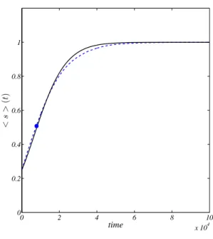
In [7] authors proved that (5) can be analytically solved once we provide the initial distribution of node strengths (see Appendix A for a short discussion of the involved methods). Assuming si(0) to be uniformly distributed in [0, 1/2], we get the following exact solution (see Fig. 2):
< s > (t) = e γ2t eγ2t− 1− 2eγ2t (eγ2t− 1)2log µ eγ2t+ 1 2 ¶ , (6)
aLet us observe that the affinity may not be symmetric and thus the inspected social network will
be directed. One has thus to distinguish between In–degree, kin, being the number of incoming
edgesof a vertex and Out–degree, kout, being the number of its outgoing edges. In the following
Using similar ideas we can prove [7] that the variance σ2 s(t) =< s2> − < s >2 is analytically given by σ2(t) = 2e 2γ2t (eγ2t− 1)2(eγ2t+ 1) − 4e2γ2t (eγ2t− 1)4 · logµ e γ2t+ 1 2 ¶¸2 . (7) The comparison between analytical and numerical profiles is enclosed in Fig. 2, where the evolution of < s > (t) is traced. Let us observe that here γ2 will serve as a fitting parameter, when testing the adequacy of the proposed analytical curves versus direct simulations, instead of using its computed numerical value [10]. The qualitative correspondence is rather satisfying, so confirming the correctness of the analytical results reported above.
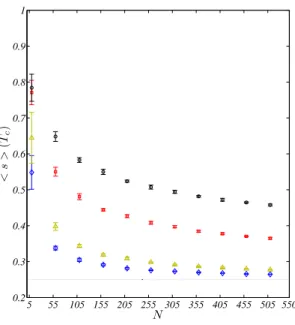
Assume Tc to label the time needed for the consensus in opinion space to be reached. Clearly, Tcdepends on the size of the simulated systemb. From the above relation (6), the average node strength at convergence as an implicit function of the population size N reads:
< s > (Tc(N )) = e γ2(N )Tc(N ) eγ2(N )Tc(N )− 1− 2eγ2(N )Tc(N ) (eγ2(N )Tc(N )− 1)2log µ eγ2(N )Tc(N )+ 1 2 ¶ , (8) where we emphasized the dependence of γ2 and of Tc on N . However, as al-ready observed γ2(N ) = O¡N−2¢ and Tc(N ) = O (Na), with a ∈ (1, 2). Hence γ2(N )Tc(N ) → 0 when N → ∞ and thus < s > (Tc(N )) is predicted to be a decreasing function of the population size N , which converges to the asymptotic value 1/4, the initial average node strength (see Fig. 3), given the selected initial condition. In sociological terms this means that even when consensus is achieved the larger the group the smaller, on average, the number of local acquaintances. This is a second conclusion that one can reach on the basis of the above analytical developments.
2.2. Small world
Several social networks exhibit the remarkable property that one can reach an arbi-trary far member of the community, via a relatively small number of intermediate acquaintances. This holds true irrespectively of the size of the underlying network. Experiments [20] have been devised to quantify the “degree of separation”in real system, and such phenomenon is nowadays termed the “small world”effect, also referred to as the “six degree of separation”.
On the other hand several, models have been proposed [24, 21] to construct complex networks with the small world property. Mathematically, one requires that the average shortest path grows at most logarithmic with respect to the network size, while the network still displays a large clustering coefficient. Namely, the network has an average shortest path comparable to that of a random network, with the same
b
In [3, 8] it was shown that Tcscales faster than linearly but slower than quadratically with respect
number of nodes and links, while the clustering coefficient is instead significantly larger.
In this section we present numerical results aimed at describing the time evo-lution of both the average shortest path and the clustering coefficient of the social network emerging from the model. As before, the parameters are set so to induce the convergence to a consensus state in the opinion space.
We will be particularly interested in their values at consensus, terming the asso-ciated values respectively < ℓ > (Tc) and C(Tc) once the consensus state has been achieved.
In Fig. 4 we report these quantities (normalized to the homologous values es-timated for a random network with identical number of nodes and links) versus the system size, computed using the adjacency matrix obtained by binarizing the affinity matrix as prescribed in Remark 1 using a value of αf equal to 0.5 . The (normalized) clustering coefficient is sensibly larger than one, this effect being more pronounced the smaller the value of αc. On the other hand the (normalized) average shortest path is always very close to 1.
Based on the above we are hence brought to conclude that the social network emerging from the opinion exchanges, has the small world property. This is a re-markable feature because the social network evolves guided by the opinions and not result from an artificially imposed recipe. The implications of these findings on real social networks deserve to be further and deeply analyzed.
2.3. Weak ties
Social networks are characterized by the presence of hierarchies of well tied small groups of acquaintances, that are possibly linked to other such groups via “weak ties” [12]. According to Granovetter [15] these weak links are fundamental for the cohesion of the society, being at the basis of the social tissue, so motivating the statement “the strength of weak ties”. Such phenomenon has been already shown to be relevant in social technological networks [22].
In general any structured social tissue, can be generically decomposed into com-munities (internally connected subgroups of affine individuals) weakly linked to-gether. In the following, we invoke a strong working hypothesis and require that agents belonging to each selected subgroup of size m are indeed all linked together, thus defining a clique [1] of size m, hereafter simply m-clique.
The degree of cliqueness of a social network is hence a measure of its cohe-sion/fragmentation: the presence of a large number of m-cliques together with very few, m′-cliques, for m′ > m, means that the population is actually fragmented into small pieces, of size m not strongly interacting each other.
We are interested in studying such phenomenon within the social network emerg-ing from the opinion dynamics model here considered, still operatemerg-ing in consensus regime. To this end we proceed as follows. We introduce a cut–off parameter αf used to binarize the affinity matrix, which hence transforms into a an adjacency
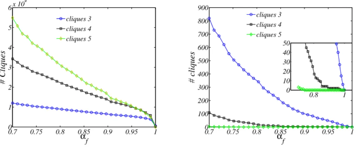
matrix a. More precisely, agents i and j will be connected, i.e. aij = 1, if and only if αij ≥ αf. Once the adjacency matrix is being constructed, we compute the number of m–cliques in the network; more precisely, because a m′–clique contains several m–cliques, with m′ > m, to have a precise information about the network topology, we count only maximal m–cliques, i.e. those not contained in any m′–cliques with m′ > m. Let us observe that this last step is highly time consuming, being the clique problem NP-complete. We thus restrict our analysis to the cases m ∈ {3, 4, 5}.
For small values of αfthe network is almost complete, while for large ones it can in principle fragment into a vast number of finite small groups of agents. As reported in the inset of right panel of Fig. 5, for αf ∼ 1 only 3–cliques are present. Their number rapidly increases as αf is lowered. On the other hand for αf ∼ 0.98 few 4– cliques emerge while 5–cliques appear around αf ∼ 0.73. This means that the social networks is mainly composed by 3–cliques, i.e. agents sharing high mutual affinities, that are connected together to form larger cliques, for instance 4 and 5–cliques by weaker links, i.e. whose mutual affinities are lower than the above ones.
Results reported in left panel of Fig. 5 show that for specific parameter values, still falling into the class deputed to the consensus dynamics, the model does not present the weak ties phenomenon: 3, 4 and 5-cliques are all present at the same time for large values of αf. This is an important point that will deserve future investigations. We also stress that the absence of weak ties could result from our specific definition of sub-community, where all agents need to be mutually linked. Weak ties could still be present and link local agglomerates, this latter displaying a more rarefied distribution of internal connections.. Let us remark that the different regimes as highlighted in Fig. 5 can be ultimately traced back to the distinct choices for the social temperature.
3. Conclusion
Social system and opinion dynamics models are intensively investigated within sim-plified mathematical schemes. One of such model is here revisited and analyzed. The evolution of the underlying network of connections, here emblematized by the mutual affinity score, is in particular studied. This is a dynamical quantity which adjusts all along the system evolution, as follows a complex coupling with the opin-ion variables. In other words, the embedding social structure is adaptively created and not a priori assigned, as it is customarily done. Starting from this setting, the model is solved analytically, under specific approximations. The functional depen-dence on time of the networks mean characteristics are consequently elucidated. The obtained solutions correlate with direct simulations, returning a satisfying agree-ment. Moreover, the structure of the social network is numerically monitored, via a set of classical indicators. Small world effects, as well weak ties connections, are found as an emerging property of the model. It is remarkable that such proper-ties, ubiquitous in nature, are spontaneously generated within a simple scenario which accounts for a minimal number of ingredients, in the context of a genuine
self-consistent formulation.
Appendix A. On the momenta evolution
The aim of this section if to present and sketch the proof of the result used to study the evolution of the momenta of the affinity distribution. We refer the interested reader to [7] where a more detailed analysis is presented in a general setting.
For the sake of simplicity, let us label the N (N − 1) affinities values αij by xl, upon assigning a specific re-ordering of the entries. Hence ~x is a vector with M = N (N − 1) elements. As previously recalled (5), we assume each xl to obey a first order differential equation of the logistic type, once time has been rescaled, namely:
dxl
dt = xl(1 − xl) . (A.1) The initial conditions will be denoted as x0
l.
Let us observe that each component xl evolves independently from the others. We can hence imagine to deal with M replicas of a process ruled by (A.1) whose initial conditions are distributed according to some given function. We are interested in computing the momenta of the x variable as functions of time and depending on the initial distribution. The m-th momentum is given by:
< xm> (t) = (x1(t)) m
+ · · · + (xM(t))m
M , (A.2)
and its time evolution is straightforwardly obtained deriving (A.2) and making use of Eq. (A.1): d dt < x m> (t) = 1 M M X i=1 dxm l dt = m M N X l=1 xm−1l dxl dt = m M N X l=1 xm−1l xl(1 − xl) = m¡< xm> − < xm+1>¢ . (A.3) To solve this equation we introduce the time dependent moment generating func-tion, G(ξ, t), G(ξ, t) := ∞ X m=1 ξm< xm> (t) . (A.4) This is a formal power series whose Taylor coefficients are the momenta of the distribution that we are willing to reconstruct, task that can be accomplished using the following relation:
< xm> (t) := 1 m! ∂mG ∂ξm ¯ ¯ ¯ξ=0. (A.5)
By exploiting the evolution’s law for each xl, we shall here obtain a partial differential equation governing the behavior of G. Knowing G will eventually enable
us to calculate any sought momentum via multiple differentiation with respect to ξ as stated in (A.5).
On the other hand, by differentiating (A.4) with respect to time, one obtains : ∂G ∂t = X m≥1 ξmd < x m> dt = X m≥1 mξm¡< xm> − < xm+1>¢ , (A.6) where used has been made of Eq. (A.3). We can now re-order the terms so to express the right hand side as a function of G c and finally obtain the following non–homogeneous linear partial differential equation:
∂tG − (ξ − 1)∂ξG = G
ξ . (A.7)
Such an equation can be solved for ξ close to zero (as in the end of the procedure we shall be interested in evaluating the derivatives at ξ = 0, see Eq. (A.5) ) and for all positive t. To this end we shall specify the initial datum:
G(ξ, 0) = X m≥1
ξm< xm> (0) = Φ(ξ) , (A.8) i.e. the initial momenta or their distribution.
Before turning to solve (A.7), we first simplify it by introducing
G = eg namely g = log G , (A.9) then for any derivative we have ∂∗G = G∂∗g, where ∗ = ξ or ∗ = t, thus (A.7) is equivalent to
∂tg − (ξ − 1)∂ξg = 1
ξ, (A.10)
with the initial datum
g(ξ, 0) = φ(ξ) ≡ log Φ(ξ) . (A.11)
cHere the following algebraic relations are being used:
ξ∂ξG(ξ, t) = ξ X m≥1 mξm−1< xm>= X m≥1 mξm< xm> , and ξ∂ξ G(ξ, t) ξ = ξ∂ξ X m≥1 ξm−1< xm>= ξ X m≥1 (m − 1)ξm−2< xm> = X m≥1 (m − 1)ξm−1< xm>
Renaming the summation index, m − 1 → m, one finally gets (note the sum still begins with m = 1): ξ∂ξ G(ξ, t) ξ = X m≥1 mξm< xm+1> .
This latter equation can be solved using the method of the characteristics, here represented by:
dξ
dt = −(ξ − 1) , (A.12)
which are explicitly integrated to give:
ξ(t) = 1 + (ξ(0) − 1)e−t, (A.13) where ξ(0) denotes ξ(t) at t = 0. Then the function u(ξ(t), t) defined by:
u(ξ(t), t) := φ(ξ(0)) + Z t
0
1
1 + (ξ(0) − 1)e−sds , (A.14) is the solution of (A.10), restricted to the characteristics. Observe that u(ξ(0), 0) = φ(ξ(0)), so (A.14) solves also the initial value problem.
Finally the solution of (A.11) is obtained from u by reversing the relation be-tween ξ(t) and ξ(0), i.e. ξ(0) = (ξ(t) − 1)et+ 1:
g(ξ, t) = φ¡(ξ − 1)et+ 1¢ + λ(ξ, t) , (A.15) where λ(ξ, t) is the value of the integral in the right hand side of (A.14).
This integral can be straightforwardly computed as follows (use the change of variable z = e−s): λ = Z t 0 1 1 + (ξ(0) − 1)e−sds = Z e−t 1 −dz z 1 1 + (ξ(0) − 1)z, (A.16) which implies λ = − Z e−t 1 dzµ 1 z− ξ(0) − 1 1 + (ξ(0) − 1)z ¶ = − log z + log(1 + (ξ(0) − 1)z)¯¯ ¯ e−t 1 = t + log(1 + (ξ(0) − 1)e−t) − log ξ(0) . (A.17) According to (A.15) the solution g is then
g(ξ, t) = φ¡(ξ − 1)et+ 1¢ + t + log ξ − log((ξ − 1)et+ 1) , (A.18) from which G straightforwardly follows:
G(ξ, t) = Φ¡(ξ − 1)et+ 1¢ ξe t
(ξ − 1)et+ 1. (A.19) As anticipated, the function G makes it possible to estimate any momentum (A.5). As an example, the mean value correspond to setting m = 1, reads:
< x > (t) = ∂ξG¯¯ ¯ξ=0=
h
Φ′¡1 + (ξ − 1)et¢ et ξet (ξ − 1)et+ 1 + Φ¡1 + (ξ − 1)et¢ et(ξ − 1)et+ 1 − ξet
(1 + (ξ − 1)et)2 i¯ ¯ ¯ξ=0 = e t 1 − etΦ(1 − e t) . (A.20)
In the following section we shall turn to considering a specific application in the case of uniformly distributed values of affinities.
A.1. Uniform distributed initial conditions The initial data x0
l are assumed to span uniformly the bound interval [0, 0.5], thus the probability distribution ψ(x) clearly reads:
ψ(x) =½ 2 if x ∈ [0, 1/2]
0 otherwise , (A.21)
and consequently the initial momenta ared: < xm> (0) = Z 1 0 ξmψ(ξ)dξ = Z 1/2 0 2ξmdξ = 1 m + 1 1 2m. (A.22) Hence the function Φ as defined in (A.8) takes the form:
Φ(ξ) = X m≥1 1 m + 1 ξm 2m. (A.23)
A straightforward algebraic manipulation allows us to re-write (A.23) as follows: X m≥1 ym m + 1 = 1 y Z y 0 X m≥1 zmdz = 1 y Z y 0 z 1 − zdz = −1 − 1 ylog(1 − y) , (A.24) thus Φ(ξ) = −1 −2 ξlog µ 1 − ξ 2 ¶ . (A.25)
We can now compute the time dependent moment generating function, G(ξ, t), given by (A.19) as:
G(ξ, t) = ξe t (ξ − 1)et+ 1 · −1 − 2 (ξ − 1)et+ 1log µ 1 − (ξ − 1)e t+ 1 2 ¶¸ , (A.26) and thus recalling (A.5) we get
< x > (t) = e t et− 1− 2et (et− 1)2log µ et+ 1 2 ¶ (A.27) < x2> (t) = e 2t (et− 1)2+ 4e2t (et− 1)3log µ et+ 1 2 ¶ + 2e 2t (et− 1)2(et+ 1). Let us observe that < x > (t) deviates from the logistic growth to which all the single variables xi(t) do obey.
For large enough times, the distribution of the variable outputs is in fact con-centrated around the asymptotic value 1 with an associated variance (calculated from the above momenta) which decreases monotonously with time.
Let us observe that a naive approach would suggest interpolating the averaged numerical profile with a solution of the logistic model whose initial datum ˆx0 acts
dWe hereby assume to sample over a large collection of independent replica of the system under
scrutiny (M is large). Under this hypothesis one can safely adopt a continuous approximation for the distribution of allowed initial data. Conversely, if the number of realizations is small, finite size corrections need to be included [7].
as a free parameter to be adjusted to its best fitted value: as it is proven in [7] this procedure yields a significant discrepancy, which could be possibly misinterpreted as a failure of the underlying logistic evolution law. For this reason, and to avoid drawing erroneous conclusions when ensemble averages are computed, attention has to be payed on the role of initial conditions.
References
[1] Albert, R. and Barab´asi, A.-L., Statistical mechanics of complex networks, Reviews of modern physics 74(2002) 47.
[2] Amblard, F. and Deffuant, G., The role of network topology on extremism propaga-tion with the relative agreement opinion dynamics, Physica A 343 (2004) 725. [3] Bagnoli, F., Carletti, T., Fanelli, D., Guarino, A., and Guazzini, A., Dynamical
affin-ity in opinion dynamics modeling, PRE 76 (2007) 066105.
[4] Barrat, A., Barth´elemy, M., Pastor-Satorras, R., and Vespignani, A., The architecture of complex weighted networks, PNAS 101 (2004) 3747.
[5] Boccaletti, S., Latora, V., Moreno, Y., Chavez, M., and Hwang, D.-U., Complex networks: Structure and dynamics, Physics Reports 424 (2006) 175.
[6] Bordogna, C. and Albano, E., Dynamic behavior of a social model for opinion for-mation, PRE 76 (2007) 061125.
[7] Carletti, T. and Fanelli, D., Collective observables in repeated experiments of popu-lation dynamics (2008), arxiv:0810.5502v1 [cond-mat.stat-mech].
[8] Carletti, T., Fanelli, D., Grolli, S., and Guarino, A., How to make an efficient propa-ganda, Europhys. Lett. 74 (2006) 222.
[9] Carletti, T., Fanelli, D., Guarino, A., Bagnoli, F., and Guazzini, A., Birth and death in a continuous opinion dynamics model - the consensus case, EPJB 64 (2008) 285. [10] Carletti, T., Fanelli, D., Guarino, G., and Guazzini, A., Meet, discuss and trust each other: large versus small groups, in Proc. WIVACE2008 Workshop Italiano Vita Artificiale e Computazione Evolutiva (Venice, Italy, 2008).
[11] Castellano, C., Fortunato, S., and Loreto, V., Statistical physics of social dynamics, Rev. Mod. Phys. 81(2009) 591.
[12] Csermely, P., Weak links (Springer Verlag, Heidelberg, Germany, 2009).
[13] Deffuant, G., Neau, D., Amblard, F., and Weisuch, G., Mixing beliefs among inter-acting agents, Adv. Compl. Syst. 3 (2000) 87.
[14] Galam, S., A review of galam models, Int. J. Mod. Phys. 19 (2008) 409.
[15] Granovetter, M., The strength of weak ties: A network theory revised, Social Theory 1(1983) 201.
[16] Gross, T. and Blasius, B., Adaptive coevolutionary networks: a review, J.R. Soc. Interface 5(2008) 259.
[17] Holme, P. and Newman, M., Nonequilibrium phase transition in the coevolution of networks and opinions, PRE 74 (2006) 056108.
[18] Klimek, P., Lambiotte, R., and Thurner, S., Opinion formation in laggard societies, Europhys. Lett. 82(2008) 28008.
[19] Kozma, B. and Barrat, A., Consensus formation on adaptive networks, PRE 77 (2008) 016102.
[20] Milgram, S. and Traver, J., An experimental study of the small world problem, So-ciometry 32(1969) 425.
[21] Newman, M. and Watts, D., Scaling and percolation in the small-world network model, PRE 60 (1999) 7332.
and Barab´asi, A.-L., Structure and tie strengths in mobile communication networks, PNAS 104(2007) 7332.
[23] Schweitzer, F. and HoÃlys, J., Modelling collective opinion formation by means of active brownian particles, EPJB 15 (2000) 723.
[24] Watts, D. and Strogatz, S., Collective dynamics of small-world networks, Nature 393 (1998) 440.
[25] Zimmermann, M., Egu´ıluz, V., and San Miguel, M., Co-evolution of dynamical states and interactions in dynamic networks, PRE 69 (2004) 065102.
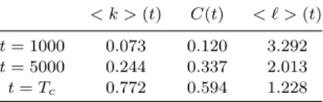
Table 1. Topological indicators of the so-cial networks presented in Fig. 1. The mean degree < k >, the network cluster-ing C and the average shortest path < ℓ > are reported for the three time configura-tions depicted in the figure.
< k > (t) C(t) < ℓ > (t) t = 1000 0.073 0.120 3.292 t = 5000 0.244 0.337 2.013 t = Tc 0.772 0.594 1.228
Fig. 1. Opinions as function of time. The run refers to αc= 0.5, ∆Oc = 0.5 and σ = 0.01. The
underlying network is displayed at different times, testifying on its natural tendency to evolve towards a single cluster of affine individuals. Initial opinions are uniformly distributed in the interval [0, 1], while α0
0 2 4 6 8 10 x 104 0 0.2 0.4 0.6 0.8 1 time < s > (t )
Fig. 2. Evolution of < s > (t). Dashed line (blue on-line) refers to numerical simulations with parameters αc = 0.5, ∆Oc = 0.5 and σ = 0.3. The full line (black on-line) is the analytical
solution (6) with a best fitted parameter γ2= 1.6 10−4. The dot denotes the convergence time in
the opinion space to the consensus state, for the used parameters affinities did not yet converge. Let us observe in fact that affinities and opinions do converge on different time scale [10].
5 55 105 155 205 255 305 355 405 455 505 550 0.2 0.3 0.4 0.5 0.6 0.7 0.8 0.9 1 N < s > (T c )
Fig. 3. Average node strength at convergence as a function of the population size. Parameters are ∆Oc= 0.5, σ = 0.5 and four values of αchave been used : (♦) αc= 0, (△) αc= 0.25, (¤)
αc= 0.5 and (°) αc= 0.75. Vertical bars are standard deviations computed over 10 replicas of
5 30 55 80 105 130 155 180 205 230 255 1 2 3 4 5 6 7 8 N C(T c )/C rnd 5 30 55 80 105 130 155 180 205 230 255 0.985 0.99 0.995 1 1.005 1.01 1.015 N < ℓ > (T c )/ < ℓ >r n d
Fig. 4. Normalized clustering coefficient (left panel) and normalized average mean path (right panel) as functions of the network size at the convergence time. Parameters are ∆Oc = 0.5,
σ = 0.5 and four values of αc have been used : (♦) αc = 0, (△) αc = 0.25, (¤) αc = 0.5 and
(°) αc= 0.75. Vertical bars are standard deviations computed over 10 repetitions. The adjacency
matrix has been obtained from the affinity matrix using αf = 0.5.
0.7 0.75 0.8 0.85 0.9 0.95 1 0 1 2 3 4 5 6x 10 4 α f # Cliques cliques 3 cliques 4 cliques 5 0.7 0.75 0.8 0.85 0.9 0.95 1 0 100 200 300 400 500 600 700 800 900 α f # cliques cliques 3 cliques 4 cliques 5 0.8 1 0 10 20 30 40 50
Fig. 5. Number of maximal 3, 4 and 5–cliques in the social network once consensus has been achieved. Parameters are N = 100, ∆Oc = 0.5, αc = 0.5. Right panel, σ = 0.5, the network
exhibits the weak ties property. Left panel, σ = 0.1, the network does not display the weak ties phenomenon.