Employee ownership as a signal of management quality

HAL Id: halshs-00534025

https://halshs.archives-ouvertes.fr/halshs-00534025

Preprint submitted on 8 Nov 2010

HAL is a multi-disciplinary open access

archive for the deposit and dissemination of sci-entific research documents, whether they are pub-lished or not. The documents may come from teaching and research institutions in France or abroad, or from public or private research centers.

L’archive ouverte pluridisciplinaire HAL, est destinée au dépôt et à la diffusion de documents scientifiques de niveau recherche, publiés ou non, émanant des établissements d’enseignement et de recherche français ou étrangers, des laboratoires publics ou privés.

Employee ownership as a signal of management quality

Nicolas Aubert, André Lapied, Patrick Rousseau

To cite this version:

Nicolas Aubert, André Lapied, Patrick Rousseau. Employee ownership as a signal of management quality. 2010. �halshs-00534025�

GREQAM

Groupement de Recherche en Economie Quantitative d'Aix-Marseille - UMR-CNRS 6579 Ecole des Hautes Etudes en Sciences Sociales

Universités d'Aix-Marseille II et III

Document de Travail

n°2010-35

Employee ownership as a signal of management

quality

Nicolas Aubert

André Lapied

Patrick Rousseau

September 2010

1

EMPLOYEE OWNERSHIP AS A SIGNAL OF MANAGEMENT QUALITY

September 2010

Nicolas AUBERT1, André LAPIED2, Patrick ROUSSEAU3

Abstract :

The employees’ decision to become shareholder of the company they work for can be a consequence of employers’ matching contribution in company stock. From a behavioral perspective, employees would regard these contributions as an implicit investment advice made by their employer. This paper adopts another viewpoint. Since employee ownership can be used as an entrenchment mechanism, we suggest that employer’s matching policy can be considered as an imperfect signal of management quality. This paper suggests that employee ownership can be used by managers to compensate their management skills to the market. It recommends that employee ownership policy should not be influenced by the managers.

Keywords: Employee ownership, corporate governance, management entrenchment.

JEL classification: G11, G32, G34, J33.

1

Corresponding author : nicolas.aubert@univmed.fr. DEFI, Université de la Méditerranée, Château La Farge – Route des Milles 13290 Les Milles (France).

2

GREQAM, IDEP, Université Paul Cézanne. 15-19 allée C. Forbin, 13627 Aix-en-Provence Cedex 1 (France).

3

CERGAM, Université Paul Cézanne. Clos Guiot Puyricard - CS 30063, 13089 Aix en Provence Cedex 2 (France).

2

1. Introduction

There are conflicting arguments regarding employee stock ownership in the academic literature. On one hand, employee ownership would enhance corporate performance through its incentive effects. Moreover, Weitzman (1984) argued that profit sharing mechanism could solve stagflation. On another hand, it would result in poor corporate governance due to the potential collusion between employee owners and management. Indeed, Blasi (1988, p. xi) remarked that employee ownership could be regarded as a revolution or a rip-off. From his point, employee ownership could be regarded as a revolution when it improves corporate performance and lead to a better workplace’s satisfaction. But it could lead to a rip-off when it is used as a management entrenchment mechanism.

These conflicting points lead us to investigate management’s motivations to offer company stock to employees. Benartzi (2001) argues that employees tend to consider management matching contribution in company stock as an implicit investment advice. He calls this phenomenon the “endorsement effect” and regards it as primarily behavioral. This paper rather regards matching contribution in company stock as a signal of management quality. From this standpoint, by choosing the level of company stock granted to employees, management would signal their type to the market. Good managers would use employee ownership as an incentive mechanism while bad managers would use it as an entrenchment mechanism.

We emphasize three main results. Firstly, we show that bad managers wish to appear as good ones by using employee ownership as an imperfect signal of their management quality. Secondly, good managers must offer higher level of employee ownership to signal themselves because of the presence of bad managers. Due to this phenomenon, bad managers have an incentive to appear as good managers, but also, good managers have an incentive to appear as bad. Thirdly, introducing prior commitments by the managers could solve this problem. From a managerial perspective, this paper suggests that employee ownership can be used by managers to compensate their management skills to the market. It recommends that employee ownership policy should defined by the board of directors before the manager is hired.

This paper proposes a sequential game where a risk neutral manager grants company stock to his risk averse employee. The remainder of the paper is organized as follows. Section 2 analyzes the literature on employee ownership incentive effects and its implication for corporate governance. Section 3 presents the model set-up. Section 4 develops the conditions

3

of the optimal contracting. Section 5 presents comparative statics analyses. Section 6 offers concluding remarks. All proofs are presented in the appendix.

2. Literature

A first body of literature on employee stock ownership focused on its positive effects on employees’ behavior. These researches tested how employee ownership affects work attitudes such as implication, involvement, satisfaction, turnover and turnover intention. Klein (1987) identified three perspectives to explain the effects of employee stock ownership on employees’ behavior: − intrinsic, − instrumental, − extrinsic. The first perspective is the intrinsic satisfaction. It states that employee ownership per se can increase employees’ commitment to the organization and its satisfaction. Empirical results gave a little support to this model. The second perspective is the instrumental satisfaction. It states that the employee owner satisfaction and commitment come from the participation in decision-making. Empirical tests assessed the relationship between employee ownership and perceived employees’ influence in decision-making and linked these perceptions with employees’ attitudes. The results of empirical studies support this model (Long, 1978; Long, 1980, Klein, 1987; Klein et al, 1988; French and Rosenstein, 1984; Buchko, 1992a, 1992b, 1993; Pendleton et al, 1998; Pendleton, 2001). The third perspective is the extrinsic satisfaction. It states that employee stock ownership is motivating when it is financially rewarding. Most of the empirical literature suggests that this model could explain employee owners’ positive attitudes (French, 1987; Klein, 1987; Rosen et al, 1986; Buchko 1992b, 1993; Gamble et al, 1999). Klein concluded this model is in line with the conclusions of the Principal-Agent Model. Since employee stock ownership is a way to motivate employees, it has effects on corporate performance. In the literature, performance is measured in terms of productivity and profitability. Kruse and Blasi (1997) reviewed all the empirical tests of employee stock ownership on performance. To sum up all the findings available, Kruse (2002) states that empirical literature considers employee stock ownership as having either a positive or null effects on performance.

Another body of literature on employee stock ownership focused on its negative effects on corporate governance. Employee stock ownership is often regarded as a powerful anti-takeover tool since it reduces the probability that a anti-takeover arises (Shivdasani, 1993; Beatty, 1995). From this standpoint, management would use employee ownership to put shares of the company in “friendly hands” (Benartzi et al, 2007). The argument is that collusion between management and employee owners is possible. Pagano and Volpin (2005) states that:

4

“managers and workers are natural allies against takeover threats” (p. 841). They conclude that: “managers offer long-term contracts to guard against raiders, and workers are willing to take action to protect their high wages” (p. 864). Employee ownership would serve as a management entrenchment mechanism. Gordon and Pound (1990) argue that many employee ownership plans were established in the US during the late 1980s explicitly to defend against takeovers. When an employee stock ownership plan is implemented, event studies report negative reaction of the financial markets in line with the management entrenchment hypothesis (Chang, 1990; Chang and Mayers, 1992; Conte et al, 1996). As a takeover defence, employee ownership could even be more powerful than poison pills or golden parachutes (Chaplinsky and Niehaus, 1994). Poison pills and golden parachutes are less used when an employee stock ownership plans is implemented (Park and Song, 1995). Rauh (2006) confirms that employee ownership has a deterrence effect on takeover probabilities. He further claims that: “Strategic corporate control motives are, therefore, one significant reason managers encourage employees to hold company stock in their defined contribution pension accounts. As laws grant managers more insulation from market discipline, the incentive for management to encourage employees to hold company stock decreases.” Brown et al (2006) find that offering matching contribution in company stock in 401(k) plans is more likely when they do not have multiple classes of stock which is an alternative mechanism to reduce takeover threats. According to them, employee ownership can then be interpreted as a mean to put shares in friendly hands to thwart takeovers.

According to the literature, employee ownership has therefore two sides: a bright one involving a better corporate performance and a dark side leading to management entrenchment. These arguments can be both regarded as management’s motives to stimulate employee ownership. In several countries such as the US, management encourages employee ownership through matching contributions in company stock or discount on stock prize. Even if Brown et al (2006) show that firms tend to take into account the effect of their matching policy on participant retirement security, it is unclear whether workers take advantage of holding their company stock. Meulbroek (2005) and Ramaswamy (2003) estimate that the cost of investing in employer’s stock is prohibitive. Since employee owners’ saving strategy seems to be irrational, financial economists investigated behavioral biases (see Benartzi et al (2007) for a review). Along with other cognitive biases, Benartzi (2001) finds that: “when the employer’s contributions are automatically directed to company stock, employees invest more of their own contributions in company stock (p. 1748)”. According to him this phenomenon is consistent with an “endorsement effect: employees interpret the allocation of the employer’s

5

contributions as implicit investment advice (p. 1748)”. Purcell (2003) confirms this effect using archival data by emphasizing that 401(k) concentration in company stock is significantly higher in companies where matching contributions are offered in company stock. Our paper is an attempt to investigate an alternative explanation of employees’ response to their employer’s policy regarding company stock. We suggest that granting company stock to employees can be interpreted as an imperfect signal on management quality.

3. The model

Consider a model with three stages involving a risk neutral entrepreneur and a risk averse employee. This employee is representative of all company employees. We thus consider all employees to have homogeneous preferences. Figure 1 illustrates the time line.

t=0 t=1 t=2

The nature chooses the management’s type k={G,B}: good (G) with a probability p0 or bad (B)

with a probability 1 – p0.

The manager defines the level of employee ownership c granted to

the employees (c ≥ 0).

The employee observes the level of

c and decides the level of effort

implemented j={H,L}: high (H) or low (L). FIGURE 1:TIME LINE

At t = 0, the nature chooses the manager’s quality. The type of the entrepreneur can either be good (G) or bad (B) with k={G,B}. The entrepreneur knows his type and the employee has an a priori probability distribution on it: P0, p0 = P0(G), 1 – p0 = P0(B), 0 < p0 < 1.

At t = 1, the entrepreneur designs the compensation system aimed at motivating the employee to expand his desired level of effort. The compensation system we investigate only consists in employee ownership. We thus consider a setup where the entrepreneur has to decide whether or not to offer company stock to his employee and the amount of it. The entrepreneur’s wealth

Wd is positive and totally invested in company stock. When employee ownership is offered to employee, it takes the form of a contribution in company stock that diminishes entrepreneur’s wealth. Suppose c to be a proportion of Ws, the positive initial employee’s wealth. cWs is the money value of company stock granted to employee. Indeed, the money value of the contribution granted to the employee is very often commensurate with the amount invested by the employee. For instance, it takes the form of a discount or a matching contribution.

6

Degeorge et al. (2004) confirmed empirically that wealthier employees are more willing to take a firm exposure.

At t = 2, the employee observes the compensation system and chooses e, the level of effort that affects the stochastic part of the return on company stock r. The employee’s expected utility is supposed to be additively separable between the gains and the disutility of effort. r is a random variable with a zero mean and a probability distribution f(r). r and k are supposed to be independent random variables. Let F(r eH) and F(r eL) be the cumulative distribution functions of company stock return conditional on high level of effort eH and low level of effort eL, we assume F(r eH) < F(reL). Therefore, the employee’s effort is productive in the sense of first-order stochastic dominance. The effort is personally costly to the employee that endures (e) the disutility that is increasing with effort. Employee’s initial wealth Ws is totally invested in a risk free asset whose rate of return is r0. If employee ownership is

granted, employee’s wealth increases by an amount cWs of company stock.

The return of company stock is then (1r j,k) for a level of effort j={H,L} and for different managers’ types k={G,B}. According to managers’ type and employees’ effort, the conditional means of the conditional distributions of the return take the following values: L,B

= , L,G =  + , H,B =  + , H,G =  +  + , with  > 0,  > 0,  > 0.

The entrepreneur’s and employee’s outcomes at the end of the game depend on the strategies they adopt. If, at some period of the game, one of the players decides to not participate, their expected utility at the end of the game is null. The agents’ expected utilities at the end of the game depend on the manager’ quality (G or B), on the level of employee ownership (c) and on the agent’s level of effort (H or L). Let’s denote ijk

V , , the manager expected utility if a contribution i={0,c} is granted, a level of effort j={H,L} is implemented according to his type

k={G,B}. The risk neutral manager maximizes the expected value of his wealth V0 ,j,k or Vc,j,k depending on whether c is granted or not:

 V0, j,k_{ W} d(1r j,k_{) f (r)drW} d(1 j,k₎  



(1)  Vc, j,k_{ (W} d cWs)(1r j,k_{) f (r)dr(W} d cWs)(1 j,k₎  



(2)

With c = 0 and c > 0, respectively, the expected utility of the employee is:



U0, j _u[W

s(1r0)](e

j₎

7  Uc, j _{ {p} 0u[Ws(1r0)cWs(1rj,G)](1p0)u[Ws(1r0)cWs(1rj,B)]} f (r)  



dr(ej₎ (4)

where u(.) is a risk averse von Neumann-Morgenstern utility function.

4. Derivation of the employee ownership contracts

4.1. Optimal contract

First, we characterize an equilibrium of the game without a minimum constraint on company’ return. A minimum constraint is introduced in the next sub-section.

Assumption 1: The employee is risk averse and cautious4.



x : u'(x)0,u''(x)0,RRA(x) xu''(x)

u'(x) 1 (A1)

This hypothesis implies:



x,[xu'(x)]'0 (5)

Assumption 2: The employee’s expected utility is strictly positive when company stock is

not granted, and effort is low:



U0,L _u[W

s(1r0)](e

L_)0

(A2)

Assumption 3: The employee’s expected utility is higher with employee ownership for a

given level of effort:

 Uc, j _{ {p} 0u[Ws(1r0)cWs(1r j,G_)](1p 0)u[Ws(1r0)cWs(1r j,B_)]}  



f (r)dr(ej_)U0, j _u[W s(1r0)](e j_{),c0,jH,L} (A3)

Lemma 1: The relation defined by (c) = Uc,H – Uc,L = (eH) – (eL) has the following properties: ω(0) = 0, and ’(c) > 0.

Proof: See the appendix.

4

8

Proposition 1: Without the constraint on the value V, under assumptions 1 to 3, for



1_[(eH_)(eL_)]c

k,kG,B there exists a unique

 c*(0,c_k], where  c_k:Wd W_s H ,k_L,k

1H,k 0, which is the Perfect Subgame Nash Equilibrium, for j = H, and k = {G, B}. Furthermore, c* is given by the following relation:



(c*)(eH_)(eL₎ Proof: See the appendix.

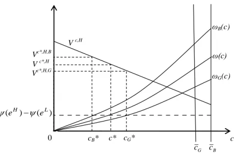
Figure 2 illustrates propositions 1 and 2. The manager selects the minimum level of c that insures a high level of effort at the intersection of ω(c) and (eH)(eL). Indeed, the higher the amount of company stock, the lower the entrepreneur’s wealth Vc,i,j

. The additional disutility bore by the employee due to a higher effort is exactly compensated by a supplementary utility of wealth. Figure 2 shows that the difference between the two levels of disutility of effort cannot be compensated above ck. Beyond ck, employee ownership

becomes too costly to the entrepreneur.

Remark 1:  c_GWd W_s  1 cB  W_d W_s  1 ₍₆₎

The two threshold constraints differ according to the two types of managers who know their type G or B whereas the employee cannot observe it.

FIGURE 2:DETERMINATION OF THE OPTIMAL EMPLOYEE OWNERSHIP CONTRACTS

0 c* ω(c) V c,H V c*,H c ) ( ) (eH  eL   G c cB cG* cB* ωB(c) ωG(c) Vc*,H,B Vc*,H,G

9

Notes. Thick lines represent (i) entrepreneur’s wealth Vc,H with the optimal contract; (ii) the maximum thresholds of company stock granted c_G and c_B; (iii) the difference of employee’s utility wealth due to a high level of effort ωk(c). Dash line represents the disutility of effort bore by the employee.

4.2. Revelation of information

Now, we introduce the condition of a minimum return for the entrepreneur. The equilibrium decision is noted ce in the sequel.

If V < Vm with Vm > 0, the entrepreneur is fired out5 and his value is fixed to 0, except if the employee’s ownership is greater than or equal to Cm, Cm > 0, or equivalently if c > cm, with

cm = Cm/Ws. In the sequel, Wd > Cm.

(i) If (Wd – c* Ws)(1 + H,G) > (Wd – c* Ws)(1 + H,B) ≥ Vm, (7) then, ce = c*, j = H, and V = Vc*,H,k = (Wd – c* Ws)(1 + H,k), for k = {G, B}.

(ii) If Vm > (Wd – c* Ws)(1 + H,G) > (Wd – c* Ws)(1 + H,B), (8) then, ce = Max(c*, cm) j = H, and V = Vce,H,k = (Wd – ce Ws)(1 + H,k), for k = {G, B}.

(iii) If (Wd – c* Ws)(1 + H,G) ≥ Vm > (Wd – c* Ws)(1 + H,B), (9) (j) for k = G, then, ce = c*, j = H, and V = Vc*,H,G = (Wd – c* Ws)(1 + H,G),

(jj) for k = B, then, ce = Max(c*, cm) j = H, and V = Vce,H,B = (Wd – ce Ws)(1 + H,B).

Remark 2: We have an increase of c for a given level of effort (H), and then a decrease of the

shareholder value. If c*>cm, the manager chooses to give c*. When ce>c*, the manager’s type is revealed to the employee.

The case (iii) corresponds to a separating equilibrium since G and B are identified.

Assumption 4: (Wd – c* Ws)(1 + H,G) ≥ Vm > (Wd – c* Ws)(1 + H,B), (A4) with c* characterized in Proposition 1.

Assumption 4 applies in the sequel.

The employee observes the value of c*, then, he can identify the type of the manager. In the case where cm > c*:

(j) If ce = c*, then k = G, (jj) If ce = cm, then, k = B.

5

This minimum return condition is consistent with the argument of Jensen and Ruback (1983). They argue that takeover target firms experience negative abnormal returns in the period prior to their acquisition.

10

The employee adapts his beliefs and then his behavior. Then, his expected utility depends now on the type k = {G, B} of the manager:

) ( ) ( )] 1 ( ) 1 ( [ ₀ , , , jk j s s k j c e dr r f r cW r W u U 



        ₍₁₀₎

and the relation (.) becomes k(c) = Uc,H,k – Uc,L,k + (eH) – (eL) since the employee is now able identify the manager’s type.

Lemma 2: The relations k(c) have the following properties: ωk(0) = 0, and k’(c) > 0. The solutions ck*, for k = {G, B}, of the equations:



_k(c_k*)(eH_)(eL₎

are such that: cB* < c* < cG *.

Proof: See the appendix.

Remark 3: Irrespective of the c_k constraint, a higher amount is required from the good manager.

Proposition 2: Under assumptions 1 to 4, for H L _G

G e  e c  )] ( ) ( [ 1  

- In the case where cm > c*, there exists a unique cke, which is the Perfect Subgame Nash Equilibrium, for j = H, and k = {G, B} such that:

(j) for k = G,

(i) If (Wd – cG* Ws)(1 + H,G) ≥ Vm, cGe = cG*, (11) (ii) If (Wd – cG* Ws)(1 + H,G) < Vm, , cGe = Max(cG*, cm), (12) In (ii), we underlines that the good manager’s wealth can now be below the Vm constraint whereas it was not possible with the contract described in the previous section.

(jj) for k = B, (i) If (Wd – cB* Ws)(1 + H,G) ≥ Vm, cBe = cB*, (13) (ii) If (Wd – cB* Ws)(1 + H,G) < Vm, , cBe = cm, (14) where  c_G*(0,c_G] and 

c_B*(0,c_G] are given by the following relation:



_k(c_k*)(eH_)(eL₎

for k = G, B.

- In the case where cm ≤ c*, there exists a unique c*[0,cG], which is the Perfect Subgame

Nash Equilibrium, for j = H, and k = {G, B}. Furthermore, c* is given by:



(c*)(eH_)(eL₎

(15)

11

Remark 4: The revelation of information increases the contribution for k = G, and decreases

the contribution for k = B, for a given level of effort H. These relations hold when the constraint c_k and the revelation of the information have an effect. This conclusion does not invalidate the previous findings. Bad managers offer a higher contribution to avoid a layoff. Because of the presence of bad managers, the level of the contribution increases. This phenomenon can be analyzed as an adverse selection problem where signaling is costly to the good managers only because of the presence of bad managers. The employee is always more demanding with good managers. This situation occurs because the disutilities of effort difference does not depend on manager’s type. Furthermore, the equilibrium is reached when this difference is equal to the expected utilities difference. This latter difference is higher for good managers (see figure 2).

4.3. Cheating and commitments

Both managers’ types have an incentive to cheat. The good and the bad managers can respectively offer the bad and the good contribution. In this situation, the equilibrium conditions do not hold any more. Let’s examine this assertion. When cG* < cm and (Wd – cG*

Ws)(1 + H,G) ≥ Vm >(Wd – cB* Ws)(1 + H,G), a bad manager has a greater expected profit if he offers the good manager’s contribution level cG* instead of cm (see Proposition 2). As for the good manager, he has a greater expected profit if he offers the bad manager’s contribution level cB* instead of the good one cG* (see Proposition 2), or if he offers cm (as a type B) instead of cG* (see Proposition 2) when cG* > cm, or if he offers cB* (as a type B) instead of cm (see Proposition 2). These substitutions are valuable in any cases except the case where type B has an incentive to cheat, that is when: cG* < cm, and (Wd – cG* Ws)(1 + H,G) ≥ Vm >(Wd – cB*

Ws)(1 + H,G).

It follows that, in any case, B gives the signal G or G gives the signal B. Both managers’ types have an incentive to choose the same behavior and the revelation is no longer possible. But this result opens the question of a second round problem: what is the optimal decision in the situation where it is possible to cheat? This question is submitted to an infinite regression phenomenon and no solution can appear without the introduction of necessarily arbitrary meta-believes.

Another way to solve the problem is to introduce commitments. The level of c can be set before the nature chose the manager’s type. His expected value is then:

12

= Wd [1 + p0j,G + (1 – p0) j,B], (16)

or:

Vc,j = p0(Wd – c Ws) (1 + j,G) + (1 – p0) (Wd – c Ws) (1 + j,B)

= (Wd – c Ws) [1 + p0j,G + (1 – p0) j,B]. (17)

Proposition 3: Under assumptions A1 to A4, for



_G1_[(eH_)(eL_)]c

there exists an unique cke, which is the Perfect Subgame Nash Equilibrium, for j = H, and

k = G, B, such that:

- In the case where cm > c*, (i) If  p₀(W_d c *W_s)(1H,G_)(W d cmWs)(1), cke = c*, (18) (ii) If  p₀(W_d c *W_s)(1H,G_)(W d cmWs)(1), cke = cm, (19) - In the case where cm ≤ c*: cke = c*.

Where c* is given by the following relation:

 (c*)(eH_)(eL₎ , and       0 , 1 p W W c s d      (20)

Proof: See the appendix.

Remark 5: According to proposition 3, a better compensation policy involving employee

ownership should be designed before the manager type is known. From a managerial perspective, this means that the stockholders in charge of hiring and controlling the manager should not leave decisions regarding employee ownership policy to the manager’s discretion. Otherwise, our conclusions show that managers are likely to use employee ownership to compensate their type. But if such a recommendation applies, employee ownership does not allow separating good managers from bad managers any more.

5. Comparative statics

To illustrate how relational contract can be used, this section provides numerical results of the model. The calibration needs the specification of the distributions of company stock returns and the employee’s utility function. We take the usual assumption of normality for the distribution and a negative exponential utility function. Given the conditions of the perfect Nash equilibrium in sub-game expounded in section 4.2 by the proposition 2 and the form of the negative exponential utility function, the analytical solution of ck* is given by

) ( ) ( ) ( ) ( ) ( _k* H,k _k* L,k *_k H L k c F c F c  e  e      , then:

13  DL,k_(c k *_)DH,k_(c k *_)(eH_)(eL₎ , k = {G, B}, where: ]} 2 ) 1 ( ) 1 [( exp{ ) ( 2 2 , 0 ,   jk s s k j ac W c r aW c D       , with j = {H, L}. (21)

In Proposition 1, the equilibrium value c* is given by:

 (c*)[ p₀FH,G_{(c*)(1p} 0)F H,B_(c*)][p 0F L,G_{(c*)(1p} 0)F L,B_{(c*)](e}H_)(eL₎ , (22)  p₀[FH,G_(c*)FL,G_{(c*)](1p} 0)[F H,B_(c*)FL,B_{(c*)](e}H_)(eL₎ (23)  p₀[DL,G_(c*)DH,G_{(c*)](1p} 0)[D L,B_(c*)DH,B_{(c*)](e}H_)(eL₎ . (24)

Proof: See the appendix.

Traditional comparative statics analysis makes it possible to emphasize several properties of the solution. Figure 3 displays the results of the simulations.

Figure 3 (a) displays the positive relationship between p0 and c*. The higher the probability of having a good manager is, the higher the amount of company stock granted to the employee. In an economy where good managers are more numerous, the employees request a higher contribution in company stock according to remark 4. If p0 = 0, c*=

* B c and if p0 = 1, c* = * G c .

Figure 3 (b) shows the relationship between α and c*,c*_G and c*_B. The α parameter makes the difference between good and bad managers. Whereas it has no effect on c*_B, it increases the value of the contribution cG* . This result confirms and reinforces the previous conclusion of

figure 3 (a) and remark 4. As the difference between bad and good managers increases, the employees become more demanding and seek to capture a higher proportion of company’s wealth. In a situation where the employees think they face good managers, they therefore ask a higher amount of company stock.

Figure 3 (c) displays the positive relationship between μ and c*,cG* and

*

B

c . The μ parameter is the company basic stock mean return. As for this chart, the more profitable is the firm, the more the employee wants to be compensated with company stock. We also notice a higher difference between cG* and c* than between

*

B

c and c*. This result emphasizes that, for a given level of μ, the employees are more sensitive to the company’s performance when the company is led by a good manager.

14

Figure 3 (d) displays the negative relationship between σ and c*, *

G

c and *

B

c . The σ parameter is the company’s returns standard deviation. According to this figure, the riskier is the firm, the less the employee wants to be compensated with company stock. We also find the comparable difference between c_G* and c* than between c*_B and c* as in figure 3 (c).

In figures 3 (c) and 3 (d), we cannot draw any conclusion from the relative positions of the lines c*,c_G* and c*_B. Although we notice that the distance between c* and c_G* is higher than the one between c* and c*_B, these differences are only determined by the value of the parameter p0 used in the simulations (i.e. 0,2). Another value would have result in a different position on the chart. For instance, if p0 = 0,5, the c* line lies exactly halfway through

* G c and * B c .

Figure 3 (e) displays the negative relationship between β and c*,c*G and

*

B

c . The β parameter makes the difference between a high and a low effort exerted by the employee. An increase of

β denotes an increase of the productivity of effort. According to this chart, this parameter has

the same negative effect on c*,cG* and

*

B

c . In fact, the employee’s effort does not depend on the manager’s type. It remains the same whatever the manager’s type is. But, as the productivity of the effort increases, the amount of company stock diminishes. In order to obtain the same return associated with a high level of effort, the manager pays the employee less because the productivity increases.

Figure 3 (f) shows the negative relationship between a and c*,c*G and

*

B

c . The a parameter is the employee’s absolute risk aversion. This parameter has the same negative effect on c*, *

G

c and c*_B because the employee’s risk aversion does not depend on the manager’s type. As the employee’s risk aversion increases, he becomes more reluctant to hold risky assets.

Figure 3 (g) shows the curvilinear relationship between Ws and c*,cG* and

*

B

c . The Ws parameter measures the employee’s wealth. Considering assumption 3, on can distinguish two different effects: a wealth effect due to the value of Ws and a scale effect related to the value of j,k. This latter effect is the more difficult to explain since it depends on the values of four different parameters i.e. α, μ, β, σ. The two former parameters are positively associated with the amount of company stock whereas the two latter are negatively associated with it (see figures 3(b) to 3(e)). As far as the increasing part of the curve, it is completely determined by the value of the parameter a i.e. the employee’s absolute risk aversion. Indeed, when the

15

simulation is run with a lower value of a (for instance 0,3), the increasing section of the curve disappears.

16 (a) (b) G c ; c*; c_B*; c*_G (c) (d) G c ; c*; cB*; * G c

Notes.Values of the parameters are: cG 0,65; p0 0,2; r0 0,05  0,1; m0,5 ; m1 ; e7,5 ; em 0,2 ; Ws 0,5 ; Wd 5 ; a0,6; 0,05; 0,05; 1

, 0



 .

17 (e) (f) G c ; c*; cB*; * G c (g) G c ; c*; c_B*; c*_G

Notes.Values of the parameters are: c_G 0,65; p₀ 0,2; r₀0,05  0,1; _m0,5 ; _m1 ; _e7,5 ; _em0,2 ; W_s 0,5 ; W_d 5 ; a0,6; 0,05; 0,05;

1 , 0



 . c*,c*Gandc*B coincide for panels (e), (f) and (g).

18

6. Concluding remarks

In this paper, we set up a model which regards employees’ compensation in company stock as an imperfect signal of management quality. This viewpoint significantly differs from the existing literature in behavioral finance. This body of literature assumes that employees invest their money in their firm because they consider their employer’s contribution in company stock as implicit investment advice. However, employee ownership is often analyzed as an entrenchment mechanism by corporate governance literature.

This paper brings about three main conclusions. Firstly, we show that employee ownership can be used by managers to compensate their actual management’s skills. Secondly, we demonstrate that higher contributions in company stock as demanded to the good managers than to the bad. This situation is similar to an adverse selection problem where the presence of bad managers makes it costly to the good managers to signal themselves. But this phenomenon comes with another problem since it incentivizes both managers’ type to hide their actual type. It is valuable for the bad managers to appear as good ones. Similarly, appearing as bad managers can also be profitable to good managers. To solve this problem, we introduce commitments which lead us to our third result. Our third main result has a normative thrust. In order to prevent managers from hiding their actual type, our model suggests that compensation mechanisms involving employee ownership should be defined before the manager’s type is known. In other words, managers should not interfere with employee ownership policy. The comparative statics section highlights several main results. First, in a situation where the employees think they face good managers, they therefore ask a higher amount of company stock. Second, for a given level of μ, the employees are more sensitive to the company’s performance when the company is led by a good manager. Third, as the productivity of the effort increases, the amount of company stock granted to the employee decreases.

Acknowledgements

We wish to thank Guillaume Garnotel for a helpful comment.

References

Beatty, A. 1995. The cash flow and informational effects of ESOP. Journal of Financial Economics 38 (2), 211-240.

Benartzi, S., 2001. Excessive extrapolation and the allocation of company stock to retirement accounts. Journal of Finance 56(5), 1747-1764.

19

Benartzi, S., Thaler, R., Utkus S., Sunstein C., 2007. The law and economics of company stock in 401(k) plans. Journal of Law and Economics 50(2), 45-79.

Blasi, J., 1988. Employee Ownership: Revolution or Ripoff?, Harper Busines, New York.

Brown J., Liang N., Weisbenner S., 2006. 401(k) matching contributions in company stock: costs and benefits for firms and workers. Journal of Public Economics 90(6-7), 1315-1346.

Buchko, A., 1992a. Effects of employee ownership on employee attitudes: a test of three theoretical perspectives. Work and Occupations 19(1), 59-78.

Buchko, A., 1992b. Employee ownership, attitudes and turnover: an empirical assessment. Human Relations, 45(7), 711-733.

Buchko, A. 1993. The effects of employee ownership on employee attitudes: an integrated causal model and path analysis. Journal of Management Studies 30(4), 633-657.

Chang, S. 1990. ESOPs and shareholder wealth: an empirical investigation. Financial Management 19(1), 48-58. Chang, S., Mayers, D., 1992. Managerial vote ownership and shareholder wealth: evidence from ESOP. Journal

of Financial Economics 32(1), 103-131.

Chaplinsky, S., Niehaus, G., 1994. The role of ESOPs in takeover contests. Journal of Finance 49(4), 1451-1470. Conte, M., Blasi, J., Kruse, D., Jampani, R., 1996. Financial returns of public ESOP companies: investors effecs

vs. manager effects. Financial Analyst Journal 52(4), 51-61.

French, J., Rosenstein, J., 1984. Employee ownership, work attitudes, and power relationships. Academy of Management Journal 27(4), 861-869.

French, J., 1987. Employee perspectives on stock ownership: financial investment or mechanism of control?. Academy of Management Review 12(3), 427-435.

Gamble, J., Culpepper, R., Blubaugh, M., 1999. ESOPs and employee attitudes: the importance of empowerment and financial value. Personnel Review 31(1), 9-26.

Gollier, C., 2008. Understanding saving and portfolio choices with predictable changes in assets returns. Journal of Mathematical Economics 44(5-6), 445-458.

Gordon, L., Pound, J., 1990. ESOPs and corporate control. Journal of Financial Economics 27(2), 525-556. Jensen, M., Ruback, R., (1983). The Market for Corporate Control: The Scientific Evidence. Journal of Financial

Economics 11(1-4), 5-50.

Klein, K. 1987. Employee stock ownership and employees attitudes: a test of three models. Journal of Applied Psychology 72(2), 319-332.

Klein, K., Hall, R., 1988. Correlates of employee satisfaction with stock ownership: who likes an ESOP most?. Journal of Applied Psychology 73(4), 630-638.

Kruse, D., Blasi, J., 1997. Employee ownership, employee attitudes, and firm perfomance: a review of the evidence, in: Lewin, D., Mitchell, D., Zaidi, M. (Eds), The Human Resources Management Handbook, Part 1. JAI Press, Greenwich, pp. 113-151.

Kruse, D., 2002. Research evidence on prevalence and effects of employee ownership, paper presented in testimony before the subcommittee on employee-employer relations, Committee on Education and

Workforce, U. S. House of Representatives, Feb. 13.

Long, R., 1978. The effects of employee ownership on organizational identification, employee job attitudes and organizational performance: a tentative framework and empirical findings. Human Relations 31(1), 29-48.

20

Long, R., 1980. Job attitudes and organizational performance under employee ownership. Academy of Management Journal 23(4), 726-737.

Pagano, M., Volpin, P. 2005. Workers, managers, and corporate control. Journal of Finance 60(2), 841-868 Park, S., Song M. 1995. Employee stock ownership plans, firm performance and monitoring by outside

blockholders. Financial Management 24(4), 52-65.

Pendleton, A., Wilson, N., Wright, M., 1998. The perception and effects of share ownership: empirical evidence from employee buy-outs. British Journal of Industrial Relations 36(1), 99-123.

Pendleton, A., 2001. Employee Ownership, Participation and Governance: a Study of ESOPs in the UK. Routledge, New York.

Rauh, J., 2006. Own company stock in defined contribution pension plans: a takeover defense?. Journal of Financial Economics 81(2), 379-410.

Rosen, C., Klein, K., Young, K., 1986. Employee Ownership in America: the Equity Solution. Lexington books, Lexington.

Shivdasani, A. 1993. Board composition, ownership structure and hostile takeover. Journal of Accounting and Economics 16(2), 148-153.

Weitzman, M., 1984. The Share Economy. Harvard University Press, Cambridge.

Appendix Proof of Lemma 1:  (c) {p0u[Ws(1r0)cWs(1r H ,G_)](1p 0)u[Ws(1r0)cWs(1r H ,B_{)]} f (r)}  



dr  {p0u[Ws(1r0)cWs(1r L,G_)](1p 0)u[Ws(1r0)cWs(1r L,B_{)]} f (r)}  



dr (25)  (c) {p0(u[Ws(1r0)cWs(1r)]u[Ws(1r0)cWs(1r)])  



(1p0)(u[Ws(1r0)cWs(1r)]u[Ws(1r0)cWs(1r)])} f (r)dr (26)

We have first ω(0) = 0. For the second property:

 '(c) {p0(Ws(1r)u'[Ws(1r0)cWs(1r)]  



Ws(1r)u'[Ws(1r0)cWs(1r)]) (1p0)(Ws(1r)u'[Ws(1r0)cWs(1r)] Ws(1r)u'[Ws(1r0)cWs(1r)])} f (r)dr (27) Let  X :Ws(1r0)cWs(1r) Y :Ws(1r0)cWs(1r) Z :Ws(1r0)cWs(1r) T :Ws(1r0)cWs(1r)

21  '(c) {p0[ XWs(1r0) c u'(X)  



YWs(1r0) c u'(Y)] (1p0)[ ZWs(1r0) c u'(Z) TWs(1r0) c u'(T)]} f (r)dr (28)  '(c)1

c {p0[Xu'(X)Yu'(Y)](1p0)[Zu'(Z)Tu'(T)] 





Ws(1r0)( p0[u'(Y)u'(X)](1p0)[u'(T)u'(Z)])} f (r)dr

(29)

Under hypothesis A1, and with:  r, X > Y, and Z > T, we have:

 r, u’(Y) > u’(X), u’(T) > u’(Z), Xu’(X) ≥ Yu’(Y), Zu’(Z) ≥ Tu’(T), and then ’(c) > 0.

Proof of Proposition 1. A Perfect Subgame Nash Equilibrium (Vc,H, Uc,H), with c > 0, must satisfy the following conditions:

The manager plays c0 if Vc,H ≥ V0,L and Vc,H ≥ 0.

The employee chooses the level of effort k = H if Uc,H ≥ Uc,L and Uc,H ≥ 0.

First, by assumption 2, when c = 0, the expected utility of employee is strictly positive with the level of effort j = L, and strictly greater than the value obtained with j = H, because (eH) > (eL) > 0. Therefore, participation of the employee in the firm is optimal. Then,

Uc,H ≥ Uc,L and Uc,L ≥ U0,L (by assumption 3), implies Uc,H ≥ 0.

Second, the entrepreneur’s exit cannot be an equilibrium because, V0,L is always possible, as it is stated in the first point, and it is strictly positive. Then, Vc,H ≥ V0,L implies Vc,H ≥ 0.

Third, with



(c*)(eH_)(eL₎

, and the lemma 1, the condition

 1_[(eH_)(eL_)]c k,kG,B, implies  c*ck. Furthermore,  c*c_k:Wd W_s H,k_L,k 1H ,k (Wd c *Ws)(1 H,k_)W d(1 L,k_)Vc*,H ,k _V0,L,k (30) and then, we have: Vc*,H,k ≥ V0,L,k, for any k.

Fourth, Uc,H ≥ Uc,L is equivalent to



(c)(eH_)(eL₎

This characterize a positive Perfect Subgame Nash Equilibrium c*, with an equality in the preceding relation.

Proof of Lemma 2. The properties of the functions k(c) result of a straightforward adaptation of the proof of Lemma 1.

Furthermore,  _G(c) {u[W_s(1r₀)cW_s(1r)]u[W_s(1r₀)cW_s(1r)]} f (r)  



dr (31)

22  _B(c) {u[W_s(1r₀)cW_s(1r)]u[W_s(1r₀)cW_s(1r)]} f (r)  



dr (32) Let  X :W_s(1r₀)cW_s(1r) Y :W_s(1r₀)cW_s(1r) a :cW_s 

_G(c) [u(Xa)u(Ya)] f (r)  



dr  _B(c) [u(X)u(Y)] f (r)  



dr with X > Y.

As u(.) is a strictly concave function, for any r, and for any strictly positive a,

u(X + a) – u(Y + a) < u(X) – u(Y), and then, G(c) < B(c), for any positive c. With (c) = p0G(c) + (1 – p0) B(c), and the preceding equation, we have:

cB* < c* < cG*.

Proof of Proposition 2. First, when cm ≤ c*, with the condition



_G1_[(eH_)(eL_)]c G, the

inequalities



cG cB and cB* < c* < cG* (Lemma 2), without revelation, the equilibrium is obtained as in Proposition 1.

Second, when cm > c*, cG* and cB* are defined as c* in Proposition 1, with G(.) and B(.) instead of (.). Their existence is satisfied with respect to Lemma 2 and the inequalities stated in the first point.

(j) for k = G, (i) If (Wd – cG* Ws)(1 + H,G) ≥ Vm, cGe = cG*, (ii) If (Wd – cG* Ws)(1 + H,G) < Vm, , cGe = Max(cG*, cm). (jj) for k = B, (i) If (Wd – cB* Ws)(1 + H,G) ≥ Vm, cBe = cB*, (ii) If (Wd – cB* Ws)(1 + H,G) < Vm, , cBe = Max(cB*, cm) = cm.

Proof of proposition 3. First, the condition Vc,H ≥ V0,L is now:

 cc :Wd W_s p₀(H ,G_L,G_)(1p 0)( H ,B_L,B₎ 1 p₀H,G_(1p 0) H,B  W_d W_s  1, p0 (33) Second, when cm > c*, for c = c*, the expected value of the entrepreneur is:

23

and for c = cm, the expected value of the entrepreneur is:



Vcm,H (W

d cmWs)(1).

Then, if Vc*,H ≥ Vcm,H, the optimal choice is c*, and if Vc*,H < Vcm,H the optimal choice is cm. Third, if cm ≤ c*, the optimal choice is c*.

These results are a direct adaptation of Proposition 1 and 2.

Application with a negative exponential utility function

This function is defined up to a positive linear transformation: u(w) =  v(w) + , and must satisfy the following normalization6: u(0) = 0. Then,  = , and, without lost of generality, we take  = 1. Therefore, in the sequel, the utility is7: u(w) = 1 – exp(– aw).

Let:  Fj,k_{(c) : u[W} s(1r0)cWs(1rj,k)] f (r)dr  



, (34)

and we suppose that f(.) is a centered normal density with variance 2. Then:

 Fj,k_{(c) : f (r)dr}  



 f j,k_(r;c)dr  



1 f j,k_(r;c)dr  



, where:  f j,k_{(r;c) :exp{a[W} s(1r0)cWs(1r j,k_)]} 1  2 exp  r2 22        f j,k_(r;c) 1  2 exp{a[Ws(1r0)cWs(1 j,k_{)]}exp(acW} sr)exp  r2 22      . (35) Let us define:  Dj,k_{(c) :} f j,k(r;c)

(x) , where (x) is a normal density with mean mx and variance x

2 ,  Dj,k_{(c)(x)D}j,k_(c) 1 _x 2 exp  (xm_x)2 2_x2        Dj,k_{(c)(x)D}j,k_(c) 1 _x 2 exp  m_x2 2_x2      exp xmx _x2      exp  x2 2_x2       f j,k_(r;c) . (36)

An identification term by term of this last relation, for x = r, leads to: x = , mx = – a c Ws2, and

6

Because U = 0 when the employee exert his exit option (see §1).

7

24  Dj,k (c)exp{a[Ws(1r0)cWs(1 j,k )]} exp (acWs 2₎2 22       (37)  Dj,k_{(c)exp{aW} s[(1r0)c(1 j,k_)ac2Ws2 2 ]}. We have:  Fj,k_{(c)1 f} j,k_(r;c)dr  



1Dj,k_{(c) (x)dx}  



1Dj,k_(c) . (38)