Stellar chemical clocks in the Gaia era

(1)

HAL Id: tel-01923867

https://tel.archives-ouvertes.fr/tel-01923867

Submitted on 15 Nov 2018

HAL is a multi-disciplinary open access archive for the deposit and dissemination of sci-entific research documents, whether they are pub-lished or not. The documents may come from teaching and research institutions in France or abroad, or from public or private research centers.

L’archive ouverte pluridisciplinaire HAL, est destinée au dépôt et à la diffusion de documents scientifiques de niveau recherche, publiés ou non, émanant des établissements d’enseignement et de recherche français ou étrangers, des laboratoires publics ou privés.

Stellar chemical clocks in the Gaia era

Anastasia Titarenko

To cite this version:

Anastasia Titarenko. Stellar chemical clocks in the Gaia era. Solar and Stellar Astrophysics [astro-ph.SR]. Université Côte d’Azur, 2018. English. �NNT : 2018AZUR4065�. �tel-01923867�

(2)

Indicateurs chimiques d’âge stellaire

à l’ère de Gaia

Anastasia TITARENKO

Laboratoire J-L. Lagrange - Observatoire de la Côte d’Azur

Présentée en vue de l’obtention du grade de docteur

en Sciences de la Planète et de l’Univers

de l’Université Côte d’Azur

Thése dirigée par: Alejandra Recio-Blanco

Soutenue le: 21 Septembre 2018

M. Carlos Abia

Professeur

Rapporteur

Mme.

Elisa Delgado Mena

Chercheur

Rapporteur

M. Mathias Schultheis

Astronome

Président, Examinateur

(3)

(4)

Indicateurs chimiques d’âge stellaire

à l’ère de Gaia

Jury

Président du jury et Examinateur:

Mathias Schultheis Astronome Observatoire de la Côte d’Azur

Rapporteurs:

Carlos Abia Professeur Université de Granada

(5)

(6)

Résumé

Les étoiles enregistrent le passé dans leurs âges, leurs compositions chimiques et leur cinématique. Elles peuvent fournir des contraintes détaillées sur les premières époques de la formation des galaxies, jusqu’aux redshifts supérieurs à deux (un recul d’environ 10 mil-liards d’années). En particulier, les âges stellaires sont essentiels pour la compréhension de l’histoire de la Voie Lactée et pour la comparaison avec les modèles d’évolution galactique. L’avènement de la mission spatiale Gaia ouvre la voie à l’estimation de l’âge pour de grands échantillons d’étoiles. En particulier, les méthodes basées sur l’ajustement d’isochrones peuvent être utilisées. En plus, les distances précises mesurées par Gaia permettent de développer les estimateurs d’âge indirects basés sur l’horloge d’évolution de la population stellaire. En fait, les schémas d’abondance chimique, imprimés sur les atmosphères stel-laires, représentent les conditions du gaz au moment de la formation des étoiles à des red-shifts supérieurs à deux. Les produits d’évolution chimique de différents canaux nucléosyn-thétiques peuvent donc fournir une approximation temporelle, qui, après l’étalonnage, peut être utilisé comme un estimateur d’âge.

Cette thèse est centrée sur l’utilisation d’horloge chimique particulière: l’abondance [Y/Mg]. À cette fin, les premières données astrométriques de la mission Gaia ont été com-binées avec des données spectroscopiques à haute résolution du catalogue AMBRE HARPS. Tout d’abord, l’identification des objets d’AMBRE a été améliorée grâce à la correspondance avec le catalogue 2MASS et la Gaia DR1. Au total, 6776 étoiles ont été identifiées.

Deuxièmement, afin d’obtenir des estimations précises du rapport d’abondance [Y/Mg] pour les étoiles du disque galactique, l’outil automatisé GAUGUIN, intégré à la chaîne Gaia DPAC APSIS, a été optimisé et testé. En particulier, les capacités d’estimation d’abondances chimiques ont été améliorées pour des grilles de spectres synthétiques irrégulières, couvrant une large gamme de paramètres atmosphèriques stellaires.

Troisièmement, le ratio [Y/Mg] a été estimé pour environ 2000 étoiles à partir des don-nées spectroscopiques d’AMBRE HARPS. Les erreurs internes et externes des abondances ont été soigneusement analysées. Les étoiles étudiées appartiennent principalement aux dis-ques mince et épais galactique, dans la gamme de métallicité allant de –1,0 dex à 0,5 dex.

Quatrièmement, grâce à l’estimation d’âge basée sur l’adaptation des isochrones pour 342 "turn-off" étoiles d’échantillon, la sensibilité à l’âge du rapport [Y/Mg] a été étudié. L’analyse révèle une corrélation claire entre [Y/Mg] et l’âge pour les étoiles du disque mince de différentes métallicités. Cela correspond aux études antérieures sur les étoiles de type solaire. De plus, aucune dépendance à la métallicité avec l’âge stellaire n’est détectée, donc le ratio [Y/Mg] peut être utilisé comme un indicateur fiable d’âge.

Enfin, la relation [Y/Mg] versus l’âge présente une discontinuité entre les étoiles du disque épais autour de 9–10 Gyrs. Pour ces étoiles, la corrélation est différente et a une tendance probablement plus forte avec l’âge. Cela reflète la différence dans les histoires d’évolution chimique pour les deux composantes du disque.

Keywords— étoiles: âges - étoiles: abondances - étoiles: évolution - étoiles: paramètres

(7)

(8)

Abstract

Stars record the past in their ages, chemical compositions and kinematics. They can provide unprecedented detailed constraints on the early epochs of galaxy formation, back to redshifts greater than two (a look-back time of around 10 billion years). In particular, stellar ages are crucial to the understanding of the Milky Way history and for comparison with galactic evolution models.

The advent of the Gaia space mission has opened the path to stellar age estimations for large samples of stars, in particular, based on isochrone fitting methods. In addition, Gaia precise distances allow to develop indirect age estimations based on the stellar population chemical evolution clock. In fact, the chemical abundance patterns imprinted on stellar at-mospheres represent the gas conditions at the time of the stars’ formation back to redshifts greater than two. The chemical evolution products of different nucleosynthetic channels can therefore provide a time proxy. After calibration, it can be used as an age estimator.

This thesis is focussed on the use of a particular chemical clock, the [Y/Mg] abundance. To this purpose, the astrometric Gaia mission data from the first data release was combined with high resolution spectroscopic data from the AMBRE-HARPS catalogue. First of all, the object identification of the AMBRE archival data was improved, thanks to a cross match with the 2MASS catalog, and later the Gaia DR1. In total, 6776 different stars have been identified.

Secondly, in order to obtain precise estimations of the [Y/Mg] abundance ratio for galac-tic disc stars, the automated GAUGUIN tool integrated in the Gaia DPAC APSIS chain, has been optimized and tested. In particular, the abundance estimation capabilities of the AP-SIS GAUGUIN tool have been improved for irregularly distributed synthetic spectra grids, spanning a large range in stellar atmospheric parameters.

Thirdly, the [Y/Mg] abundance ratio has been estimated for about 2000 stars from the AMBRE HARPS spectroscopic data. In addition, the internal and external errors of the abundances were carefully analysed. The studied stars belong mainly to the galactic thin and thick disc, in the metallicity range from -1.0 dex to 0.5 dex.

Fourth, thanks to the isochrone fitting age estimations of 342 turn-off stars of the sample, the age sensitivity of the [Y/Mg] ratio has been studied. The analysis reveals a clear corre-lation between [Y/Mg] and age for thin disk stars of different metallicities, in synergy with previous studies of Solar type stars. In addition, no metallicity dependence with stellar age is detected, allowing to use the [Y/Mg] ratio as a reliable age proxy.

Finally, the [Y/Mg] vs. age relation presents a discontinuity between thin and thick disk stars around 9–10 Gyrs. For thick disk stars, the correlation has a different zero point and probably a steeper trend with age, reflecting the different chemical evolution histories of the two disk components.

Keywords— stars: ages – stars: abundances – stars: evolution – stars: fundamental

(9)

(10)

Remerciements

Au cours de ces 10 dernières années j’ai étudié la physique stellaire; cette thèse marque maintenant la fin de ma vie étudiante. Je voudrais remercier tous les enseignants qui ont partagé leur expérience avec moi et, en premier lieu la directrice de cette thèse, Alejandra Recio-Blanco, pour m’avoir guidée et apporté son savoir.

Je suis reconnaissante à Thierry Lanz, Philippe Stee et le groupe administratif, en par-ticulier Betty Bonhomme, Joël Bealu, Christine Delobelle, Sophie Rousset et Catherine Blanc, pour leur aide avec les problèmes administratifs apparus pendant ces années.

Merci à Mathias Schultheis, Patrick de Laverny et Vanessa Hill pour leur disponi-bilité à discuter sur divers sujets scientifiques. J’exprime mes remerciements à Cristoph Ordenovic pour sa patience pour notre travail sur la version Java de la méthode GAUGUIN. Je remercie les membres d’équipe GAG et séminaires Lagrange pour les rencontres perti-nentes et intéressantes, pour rester au courant des nouvelles astrophysiques.

Mes remerciements à Elena Lega et Chiara Ferrari pour leur aide et leurs conseils. Merci au groupe de support technique, Daniel Kamm, Ghibaudo Jean-Philippe et Marie-Laure Miniussi, pour leurs réponses rapides et efficaces en cas de problème.

Je voudrais remercier mes collègues du bureau, Edouard Bernard et Michael Hayden, pour leur patience et leur courage de s’engager dans les dialogues parfois très étranges. Merci à tous mes fréres-en-thèse (Francesco, Govind, Camemberto, Pablo, Michael II, Emma, Sophia, Emmanuele, Marina, Rémi, Brynna, Ximena, Alvaro, Gabriele, Clément, To-bias, João, Michael, Raphael, Elena, Vitaly, Go) pour la joie de ces années.

Avec un grand plaisir je mentionne ici Laurent Galluccio, pas seulement parce qu’il m’a demandé plusieurs fois de le mettre dans la liste de remerciements, mais surtout pour son aimabilité et sa gentillesse. Un grand merci à Bernard Pichon, Serge Bonhomme, Dominique Triboire et les amis d’Ateliers et Services Techniques pour leur humour.

Je mentionne ici le groupe de la cantine, Khaled, Karima et Dominique, qui rende notre vie plus heureuse. J’apprécie Khaled pour toutes les choses qu’il m’a lancées à la tête, mais heureusement ratée.

Merci à Nathalie Nergeault et Seyna n’Diaye pour nos moments divertissants et leur aide pour certaines questions du quotidien.

Merci Eric Fossat, Michéle Pascaud, Farrokh Vakhili et Lionel Bigot pour les beaux jours passés ensemble dans les montagnes.

Merci à Sylvie de la part de la bichette pour le temps qu’on a passé ensemble.

Merci à toi, Aymeric, d’être avec moi dans les situations heureuses et moins heureuses. Merci à toi, Gilles, pour nos dialogues constructifs et pour tout ce que tu fais pour moi. Enfin, j’aimerais remercier ma famille pour son soutien et son aide dans toutes les situ-ations qui se présentent dans ma vie.

(11)

(12)

Acknowledgements

During the past 10 years I have studied stellar physics, and this thesis marks the end of my student life. I would like to acknowledge all the teachers who have shared their experience with me during these years, and first of all, the director of this PhD-project Alejandra Recio-Blanco for her guidance and mentorship during my PhD.

I am thankful to Thierry Lanz, Philippe Stee and those in administration, especially Betty Bonhomme, Joël Bealu, Christine Delobelle, Sophie Rousset and Catherine Blanc, for their help with diverse administrative problems, that have appeared during these years.

Thanks to Mathias Schultheis, Patrick de Laverny and Vanessa Hill for their avail-ability to discuss any scientific problems. In particular, I would like to express my thanks to Cristoph Ordenovic for your patience in our work on java-version of the GAUGUIN method. With a pleasure I thanks all the members of GAG group and Lagrange seminars for useful and interesting meetings, that allow to stay in the flow of modern ideas of astrophysics.

My respectable thanks to you, Elena Lega and Chiara Ferrari, for your help and advice. Thanks to technical support group, Daniel Kamm, Ghibaudo Jean-Philippe and Marie-Laure Miniussi, for their rapid answers in the case of technical issues.

I would like to thank my office mates, Edouard Bernard and Michael Hayden, for their patience and interesting conversations, of varying levels of strangeness. Thanks to all of my brothers and sisters-in-PhD (Francesco, Govind, Camemberto, Pablo, Michael II, Emma, Sophia, Emmanuele, Marina, Rémi, Brynna, Ximena, Alvaro, Gabriele, Clément, To-bias, João, Michael, Raphael, Elena, Vitaly, Go) for the fun and joy of these years.

With a pleasure I mention Laurent Galluccio here, not just because he asked many times to put his name in the acknowledgement list, but for his kind and gentle nature. Thank you Bernard Pichon, Serge Bonhomme, Dominique Triboire and friends from Workshops And Technical Services for your humour.

I can not skip the group from the canteen, Khaled, Karima and Dominique, that makes our daily lives more happy and fulfilled. I appreciate Khaled for all the things that he had thrown at me, but fortunately did not really reach the target.

Thanks to Nathalie Nergeault and Seyna n’Diaye for your help in some daily questions. Thank you, Eric Fossat, Michéle Pascaud, Farrokh Vakhili and Lionel Bigot, for some sunny days that we have spent out together in the mountains.

A lot of kisses I send to Sylvie from "la bichette".

Thank you, Aymeric, for being with me in happy and not really moments.

Thank you, Gilles, for our constructive dialogues and for that you are doing for me. Last but not least, I would like to thank my family for their support and understanding in different situations of my life.

(13)

(14)

Introduction

1.1 Historical aspects and present day context

Figure 1.1: The ESO 3.6-metre telescope at La Silla, during observations. Credit: ESO / S. Brunier

The sky plenty of stars excited humans eye from a very early epoch. The first traces of astronomical observations come from VI-IV BC, and the first names of some celestial bodies were found in a religious monument, the Pyramids, created in XXV-XXIII BC. We can find astronomical tables and lunar calendars from Babylon in II BC. In the Ancient Egypt, lunar calendars with metonic cycles appear. Careful observations of celestial bodies and eclipses, dated by court astronomers in China in III-II BC, are reported. The tight relations of obser-vational astronomy, religion and daily life were exceptional for the Inca Empire (XI-XVI) and the Maya civilization (II BC - X). In addition, astronomy had a wide use in the Ancient Greece, where some cosmogonist models of the origins of our Universe were proposed.

These ancient astronomical remains amaze today by their precision and flair to explain the astronomical surrounding thanks only to a few basic observations. A long way has been made since then, arriving nowadays, through the progressive development of observational instruments and fundamental physics, to the modern view of the Universe.

Obviously, many important questions remain to be solved and, among them, the forma-tion of our galaxy, the Milky Way, is of the most fundamental ones. Galactic Archaeology aims at unveiling the history of the Milky Way by analysing stars, just as the history of life was deduced from examining rocks. Stars record the past in their ages, compositions and kinematics and can provide unprecedented detailed constraints on the early phases of galaxy formation, back to redshifts greater than two (a look-back time of 10 billion years). In partic-ular, in some cases the chemical abundance patterns imprinted on stellar atmospheres could

(18)

1.2. Stellar components of the Galaxy 3

reflect the gas conditions at the time of the stars formation. In general the continuous pro-ducing of different chemical elements due to thermonuclear burning should be taken into account. The "chemical tagging" approach (Freeman and Bland-Hawthorn,2002) opens the way to the temporal sequencing of a large fraction of stars.

This thesis research is precisely dedicated to stellar dating through the analysis of the stars chemical abundances. Since the advent of stellar astrophysics, the estimation of stellar ages has been a crucial challenge with many fundamental implications. Starting with the historical debate around the age of our Sun, stellar ages have been recognized as clocks of the evolving Universe that we wish to understand. They are the basis of stellar evolution studies, of the stellar properties coded in chemical evolution analysis, and more generally, a key piece of information of our understanding of any stellar population. Numerous dating methods have been developed, based on different physical processes and models. Nuclear cosmochronol-ogy (Hoyle and Fowler(1960),Bland-Hawthorn and Freeman(2014)), isochrone fitting (first discovered bySchaltenbrand(1974),Luri et al.(1992),Valls-Gabaud(2014)), asteroseismol-ogy techniques (Pesnell(1987), Guzik et al.(2000)) and more indirect chemical proxies of stellar age have been used and applied to very different samples of stars. In particular, for Galactic Archaeology studies, dating techniques applicable to large numbers of objects are crucial. In this framework, secondary clocks, like chemical abundance age proxies ([Y/Mg] one was used in this work) are important to extend the possibility of stellar dating i) out-side the sphere of precise distance estimations and ii) to stars in different stellar evolutionary stages.

1.2 Stellar components of the Galaxy

In the current cosmogony paradigm, a Λ-Cold Dark Matter (ΛCDM) cosmology, dark matter and dark energy shape the large-scale expansion of the Universe, while on smaller scales, tiny initial fluctuations grow into large dark matter halos, where galaxies like ours form. Galaxies grow through a sequence of merger and accretion events and, inside galaxies, baryon matter aggregates to form stars. However, the interplay between gas, stars, black holes, dark matter and dark energy has only started to be understood.

The historical vision of the galactic stellar populations in galaxies was introduced by

Baade(1946). He defined three main categories, based on the physical distribution of the stars in space, their position in the Hertzsprung-Russell diagram (Fig. 1.4), and the stellar motion about the galaxy. Population I contains stars in the galactic disk. It is a young pop-ulation having a high rotation velocity, small velocity dispersion of their velocities (around 10-15 km/s), and high abundance of metals. Population II is composed of old stars (like glob-ular clusters in the halo), having low rotational velocity, high velocity dispersion (around 75 km/s) and low metal abundances. Population III is theoretically predicted to be composed of first stars that were generated after the Big Bang, basically consisted of hydrogen (p-p chain). They are predicted to be very massive and thus quickly exploded. The modern view

(19)

on stellar populations is much complex that a simple separation in three categories.

Figure 1.2: Schematic representation of components of our Galaxy.

Later on,Eggen et al. (1962) were the first to show that it is possible to study Galactic archaeology using stellar abundances and dynamics. They inferred that the Galactic metal-poor stars reside in a halo that was created during the rapid free-fall collapse of a isolated protogalactic cloud shortly after it decoupled from the universal expansion. This picture was challenged bySearle and Zinn(1978), who, studying globular clusters, suggested a halo built up over an extended period from independent fragments. The ideas of galaxy formation via hierarchical aggregation of smaller elements from the early Universe fit in easily with the view of a Galaxy formed from small fragments. Although the hierarchical model may be fundamentally different from the collapse model, it may have a few features in common. It is not unlikely that, early on in the history of the Galaxy, there was a phase which could be described as a fast dissipative collapse, but which was triggered by gas-rich mergers (Brook et al. 2004), rather than by the collapse of a giant gas cloud. Collisionless minor mergers are also proposed today to play a role in the formation of our Galaxy (Toomre,1977) as well as external gas accretion from filaments of the cosmic web and internal secular processes (Kormendy and Kennicutt,2004).

In this framework, the Milky Way is defined today as a late-type spiral, conventionally decomposed into: (i) a central bar – bulge that extends out to ∼3 kpc; (ii) a nearly spherical halo that extends out to of order 100 kpc and is studded with globular clusters; (iii) a disk that defines the Galactic plane and is probably confined to radii R less 15 kpc. The disk is often decomposed into two components, a metal rich thin disk, in which the density falls with distance Z from the plane exponentially with scale height 300 pc and a more metal poor thick disk, which is characterised by a vertical scale height 700 pc (Kordopatis et al.,2011).

(20)

1.2. Stellar components of the Galaxy 5

The thin disk is patterned into spiral arms but even now, the final word on the number and positioning of the arms present has not been spoken. Beyond the Sun the thin disk is warped.

1.2.1 The thin and the thick disks

Figure 1.3: Abundance ratios [α/Fe] vs. [Fe/H].

On the left: the blue triangles refer to the thick disk, red circles to the thin disk, magenta squares to the halo, the green asterisks and the black crosses to the transition stars between thin-thick and thick-halo, respectively. The black dashed curve separates the stars with high-/low α content. Credit:Adibekyan et al.(2012).

On the right: Same as the left panel but colour coded by age (the larger implies older). Credit:

Haywood et al.(2015).

Yoshii(1982) and thenGilmore and Reid(1983) found that the vertical number density gradient of stars in the Solar neighbourhood could not be fit by a single exponential. Instead, the density was well described by a two-component fit, one with a short scale height and one with a larger scale height. These two components became known as the thin and thick disks respectively.

The range of iron abundances in thick disk stars lies within [Fe/H] from around –1.0 to –0.5 dex, to be compared to the younger thin disk within [Fe/H] from around –0.5 to +0.3 dex. The geometrical scale heights are about 900 pc for thick disk and 300 pc for thin disks (Jurić et al.(2008)). In comparison to the thin disk, the stellar populations of thick disk have higher dispersion in vertical kinematics, older stellar ages (Masseron and Gilmore,2015) and higher ratio α-element abundances to iron content in sub-solar metallicity range (Fuhrmann

(1998),Bensby et al.(2003),Adibekyan et al.(2013),Recio-Blanco et al.(2014)).

Since the first works highlighting the existence of the Milky Way’s thin–thick disk di-chotomy, the study of the structural and chemo-dynamical transition between the two disk populations has opened new pathways to constrain Galactic evolution models. Supported by the hierarchical formation of galaxies in the ΛCDM paradigm, external mechanisms have

(21)

been invoked to explain the chemo-dynamical characteristics of thick disk stars. Among them, the accretion of dwarf galaxies (Statler(1988),Abadi et al.(2003))

and minor mergers of satellites (Quinn et al.(1993),Villalobos and Helmi(2008)) heating the disk dynamically, have been proposed. Similarly,Jones and Wyse(1983), Brook et al.

(2004) and Brook et al. (2007) have proposed that the thick disk would have been formed from the collapse produced by the accretion of a gas-rich merger. On the other hand, purely internal formation mechanisms have also been proposed, such as the early turbulent phase of the primordial disk (Bournaud et al.,2009) and the stars radial migration due to resonances with the spiral structure or the bar of the Milky Way (Schönrich and Binney(2009),Minchev and Famaey(2010), Loebman et al.(2011)), although see alsoMinchev et al. (2012). The relative importance of the different proposed physical processes of evolution can now be tested with increasing robustness thanks to the Galactic spectroscopic surveys targeting the disk stars.

1.3 Stellar Ages

The advent of the Gaia space mission (Chapter 2) has opened the path to stellar age estima-tions for large samples of stars, in particular, thanks to isochrone fitting methods. In addition, Gaia precise distances allow to develop indirect age estimations based on the stellar popula-tion chemical evolupopula-tion clock. In the following, the main techniques of stellar age estimapopula-tion are presented.

1.3.1 Asteroseismology

Historically, asteroseismology was centred in the study of solar atmosphere pulsations, ex-cited and damped by a near-surface convection (Pesnell(1987),Brown et al.(1994),Gautschy and Saio (1995) &Gautschy and Saio(1996)). The oscillation frequencies depend on the properties of stellar interior. Since these are tightly linked with the mass and evolutionary status, the mass and age of a star can be estimated from the comparison of its oscillation spectrum with stellar model predictions. The physical origin of these oscillations can be found in two types of waves. First, acoustic waves (so-called pressure modes), and second, internal gravity waves (e.g., seeHoudek et al.(1999),Samadi and Goupil(2001) &Samadi et al.(2001)). Asteroseismology age estimations are significant for solar-type and red-giant stars (Bedding et al.,2011), because the presence of a near-surface convection is a necessary condition for stars to show oscillations. The problems of modelling a star, in particular, the uncertainties on global parameters and chemical composition, and our misunderstanding of processes in stellar interiors (as the transport processes that may lead to core mixing and affect the model ages), put the limit on the age estimation accuracy.

(22)

1.3. Stellar Ages 7

1.3.2 Nuclear cosmochronology

This high-precision method is based on the spectroscopic abundances of heavy radioactive isotopes, taking into account the constant rate of radioactive decay, for example 238U and 232

Th (Hoyle and Fowler(1960), Butcher (1987), Hill et al. (2002), Bland-Hawthorn and Freeman(2014)). Based on the knowledge about the half-life time for these elements, the initial age of the matter from which the star was created, can be estimated. For this reason, the method can be effectively applied to old metal-poor stellar content of the Galaxy. This limitation together with a poor presence of uranium and thorium lines in the stellar spec-tra put severe limitations on the possibility to widely applying this method for the Galactic Archaeology.

1.3.3 Isochrone fitting methods

The story of the stellar ages determination for multiplicity of objects started with the use of isochrone fitting at the end of XX century. The first attempt comes fromSchaltenbrand

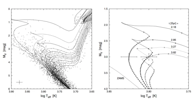
(1974). The method consists in a comparison of absolute luminosity (or magnitude) and effective temperature (or color) with theoretical models, thus estimating the nearest point of the zero-age main sequence to a star on a two-color diagram (Valls-Gabaud, 2014). These models are represented on the Hertzprung-Russel diagram with the lines, associated with populations of stars of the same age (Fig. 1.4). For this purpose different sets of isochrones can be used spanning a large range of stellar ages (Padova, Yonsei-Yale, Dartmouth etc.).

Many groups succeeded in the application of Bayesian methods to the isochrone-fitting age determination (Jørgensen and Lindegren,2005). The relative likelihood distribution of probable values of stellar ages for the star after elimination of IMF and initial metallicity rep-resents a probability for the star to have one or another stellar age inside confidence intervals. However, one of the main limitations of the method is that it can only give reliable results for the turn-off stage and the sub-giant branch. Thus, the method can be mainly applied to late A-type, F and G-dwarfs (Jørgensen and Lindegren, 2005). For other populations there may exist many age-values estimations for the same object due to the overlapping of the different isochrones.

1.3.4 Indirect chemical proxies

Apart from the primordial Big Bang nucleosynthesis that occurred during the first three min-utes of the Universe, stars themselves produce chemical elements in a chain of nuclear re-actions during their lifetimes. The type of thermonuclear rere-actions depends basically on the initial mass of the star, the type and place (core- or in layer-burning) of the thermonuclear reaction together describe evolution status of the star. Finally, produced chemical elements can be ejected into interstellar medium due to the explosion process – explosions as super-nova type Ia-II, explosions of asymptotic giant-branch stars, stellar winds, planetary nebulae etc.

(23)

Figure 1.4: The HR diagram for the synthetic sample of 2968 stars (on the left) and the loca-tion of two hypothetical observaloca-tion (on the right), the lines represent the set of isochrones of different ages. The example shows the critical case when the isochrone fitting gives a multiple solution for the same object. On the left: isochrones are for 0, 1, 2,..., 8, 10, 12 and 15 Gyr. On the right: the symbols along isochrones show where initial mass is a multiple of 0.01 Msun. Credit: Jørgensen and Lindegren(2005)

The processes of nucleosynthesis pass through hydrogen burning (the proton-proton chain or the CNO-cycle), helium (α-process), carbon, neon, oxygen and silicon burnings. Dur-ing these processes the elements up to iron and nickel can be created. Heavier elements can be created by neutron capture processes (slow neutron capture "s-process") or during explosion, as supernovae (the rapid neutron capture "r-process", the rapid proton capture process "rp-process", and the proton capture "p-process"), which results in the nuclei photo-disintegration.

As the time scales of the various nucleosynthetic processes are different, the chemical abundance ratio of two elements produced by two different channels provides a time estimate with respect to the chemical enrichment of the studied population. Indirect chemical age proxies have been used for galactic archaeology studies in the last decades, their precision and applicability domains (e.g. metallicity and age intervals) are very badly constrained. The arrival of precise distances from the Gaia mission (Chapter 2) allows today to analyse them and calibrate them in detail. In addition, high-resolution stellar spectra of different stellar types are nowadays available thanks to big spectroscopic surveys (as for example, Gaia-ESO Survey, RAVE, APOGEE,...). They allow to determine stellar abundances with a high precision, using different algorithms and reference data (See Chapter 3, Chapter 4). This amount of spectroscopic data opens a new epoch of precise stellar dating for big samples of stars, based on the calibration of different chemical abundances with stellar ages (see Chapter 6).

(24)

1.3. Stellar Ages 9

[α/Fe] abundance ratio.

α-elements are predominantly synthesized in high-mass, very short-lived stars, and are ejected by type II supernova explosions (SN II). Iron is produced by both SN II and type I super-novae (SN Ia), whose binary progenitors are believed to have a longer pre-explosion lifetime of typically one billion years (1 Gyr). Comparing the relative abundances of the α-elements and iron provides a measure of the SN Ia/SN II ratio, and in turn a clock. In the galactic disk, the distribution of [α/Fe] versus metallicity plane shows bimodal distribution, that is asso-ciated with stellar thick and thin disks (Adibekyan et al.(2012),Recio-Blanco et al.(2014). Thick disk stars have higher [α/Fe] abundances than thin disk stars of the same metallicity, showing also a faster evolution of their [α/Fe] abundance with time (Haywood et al.(2013),

Hayden et al.(2017)).

[C/N] abundance ratio.

Carbon and nitrogen are expected to be good indicators of stellar masses (Masseron and Gilmore(2015),Martig et al.(2016)). A star arrived on the giant branch, has its convective envelope extended deep inside. These convective movements bring processed through the CNO-cycle material up to the stellar surface (so-called "dredge-up"). As a result of such convective mixing, a change in the [C/N] abundance ratio at the stellar surface is observed (Iben(1965), Salaris and Cassisi(2005)). The final [C/N] ratio at the surface depends on the stellar mass, because the [C/N] abundance ratio in the core and the depth reached by the dredge-up depend on stellar mass. Since mass and age are closely related for stars on the giant branch, it makes the [C/N] ratio a rather good proxy of stellar ages (Salaris and Cassisi,

2005).

[Y/Mg] abundance ratio.

Yttrium is known to be mainly produced by s-processes in the asymptotic giant branch stage of intermediate and low mass stars. On the other hand, magnesium, as an α-process ele-ment, is produced by SN type II in a shorter time scale. That makes the [Y/Mg] abundance ratio another good proxy for stellar age dating. Contrary to the method based on the [C/N] abundance ratio, the [Y/Mg] ratio does not require additional assumptions on internal stellar structure. Since the studies ofda Silva et al.(2012),Nissen(2015),Spina et al.(2016),Tucci Maia et al.(2016), and the recent work ofAnders et al.(2018), a correlation of [Y/Mg] with stellar age for solar twins has been noticed. In the work ofFeltzing et al.(2017) they studied the relation for dwarf stars in the Solar neighbourhood in a wider range of metallicities, and

Slumstrup et al.(2017) find that this relation works also for solar metallicity stars over the helium-core-burning phase. Nevertheless those pioneer studies, the actual precision and va-lidity domain of the [Y/Mg] ratio as an age estimator is largely unknown. One of the goals of the present thesis is the study of [Y/Mg] abundance ratio age sensitivity in a wide range of metallicities. More precisely, the work is focussed on thin and thick disk stars for which Gaia astrometry data are very precise.

(25)

1.4 Spectroscopy of stellar atmospheres

The stellar atmosphere is considered to be a conservative system of gas under an equilibrium of macroscopic parameters. It can be modelled in 1D approximation as a sequence of flat parallel thin layers. The radiation transfer equation in this case could be written as: dIν/dτν = –Iν+ Sν, where ν is a chosen frequency, Iν is an intensity, τν =

z R

0

σ ds is an optical depth at chosen frequency and represents a measure of the extinction coefficient with an atmosphere depth, and Sν = jν/κν is a source function, defined as a ratio of the coefficients of emission to absorption. Then, the flux will be simply an integration of the intensity Iν in solid angle ω in a chosen direction θ per unit of time and frequency: fν =R Iνcosθ dω.

1.4.1 Continuous spectra

In stellar physics the source function plays a key role, as far as its form represents that stars’s continuous spectrum. The main source of opacity for different stars depends on its temper-ature: for hot stars it will be the ionization of neutral atoms of hydrogen HI, for solar type – negative hydrogen ions −H together with atoms of Si and metals, and for cold stars the increasing number of numerous molecular lines will be important. The veracity of the ap-proximation that the stellar atmospheres are in thermodynamic equilibrium is well confirmed by the fact that for those stars the source function is quite similar to the Planck function:

Sν = Bν(T ) = (2hν3/c2) (exp(hν/(kT ) − 1)−1,

where c is the speed of light (2.998×1010cms−1), h = 6.626×10−27eV.s is the Planck con-stant, k = 8.62×10−5 eV K−1 is the Boltzman constant. Considering this, the concept of effective temperature of the star was introduced as the temperature of a black body with the same size and luminosity as the star have: Fstar = σTef f, where Fstar is a total stellar flux, and σ = 5.670×10−8W/(m−2K−4) is the Stefan-Boltzman constant.

1.4.2 Spectral lines

Spectral lines are narrow regions (∆λ λ) in the spectra with the amplified intensity of the radiation (emission lines) or either weakened intensity of the radiation (absorption lines) compared to the continuous spectrum. The origin of spectral lines is mostly transitions of atoms, ions, molecules and atomic nuclei from one to another energy level.

The presence of spectral lines in stellar spectra means that the atmosphere is absorbing more radiation at those frequencies. For those frequencies the radiation comes from higher and less dense stellar atmosphere layers. There is no equilibrium between radiation and matter, and the radiation is damped due to the transition of the atoms from one energy level to another. This is the way how absorption spectral line appears.

An equivalent width of spectral line is a width of the rectangle with area that equals to the one in the spectral line. This concerns a plot of stellar flux versus wavelength. The

(26)

1.4. Spectroscopy of stellar atmospheres 11

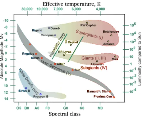
Figure 1.5: Hertzsprung-Russell diagramm. Within the same sequence, there are smooth transitions of the parameters of the stars (mass, age, diameter, luminosity, temperature and other parameters.). Stars are classified according to the spectrum.

dependence of the equivalent width of the spectral line with the number of the particles on the line of sight is called the curve of growth (Fig. 1.6).

The diversity of observed stellar spectra gave birth to a classification by stellar spec-tral type (Morgan-Keenan), that shows a diversity of effective temperatures and luminosity classes (see also the next subsection). The different stellar types can be presented in the so-called Hertzsprung-Russell diagram (see the Fig. 1.5).

Broadening of stellar lines.

The observed profile of the line will be broadened due to many different effects. Apart a broadening of spectral lines, caused by finite spectral resolution of the instrument (so-called

instrumental profile) there is a list of effects, that impact in the observed profile of a spectral

line. Their identification is important because it reveals the physical conditions in stellar atmospheres.

First, a radiation damping, i.e. the energy lost of the atom due to the radiation, causes the so-called natural broadening.

Second, the Doppler effect, caused by the motion of the observed object, makes an impact in the profile of the spectral line.

Third, the pressure effects, i.e. the interaction of the atom with the surrounding particles, broad the observed profile. In this case atomic energy levels are displaced due to the action of inter-atomic electric fields (so-called Stark effect).

(27)

Figure 1.6: The curve of growth for the chemical elements as a function of its abundance. Three possible regimes – linear 1, saturation and strong lines 2 – are represented on the left panel, and their correspondence in the line profile (weak 1 and strong 2) on the right panel. Credit: (Gray,2005).

The lines can be broadened also by the so-called Zeeman effect, the presence of magnetic fields affecting the atom. It is a splitting of the energy levels of atoms, molecules, and ions due to the electrostatic field of the electron (fine structure). It caused by the spin-orbital interaction, i.e. a relativistic interaction of a particle’s spin with its motion inside a potential.

The hyper-fine structure can impact the spectral lines profile. It is a splitting of the energy

levels of atoms, molecules, and ions, due to the interaction between the magnetic field created by the electron and the magnetic moment of the nucleus. In other words, it is caused by the interaction between the state of the nucleus and the state of the electron clouds.

Spectral lines from stellar atmospheres are normally calculated under the LTE condition (the system is in the equilibrium of all macro parameters, as a temperature, pressure, energy etc). Some additional spectral line effects, caused by the disturbance of local thermodynamic equilibrium, so-called non-LTE effects, could make an impact on the form of the spectral line for the elements with even atomic number.

Chemical abundances in stellar atmospheres.

All possible components of stellar composition can be simply defined by a sum of fractional percentages of hydrogen (X = mH/M), helium (Y = mHe/M) and other chemical elements (metals, Z): X + Y + Z = 1, where miis the fractional mass of the element, M is the total mass of the system. The determination of the abundances is given by the number ratio to hydrogen: A = log(NA/NH) + 12, it represents a number of hydrogen atoms in the solar photosphere for each atom of another element of another element A. Then the stellar abundances can be referred to the ones from the Sun, and in this case it will be given in a bracket notation: [X/Fe] = log(NX/NFe)star – log(NX/NFe)sun, and will be given in units of dex. As the result of the last definition, for some practical reasons some additional ratios can be determined as: [A/Fe] = [A/H] – [Fe/H]. This ratio is widely used in astronomy and sometimes it replaces an abundance of the element to the total metal content of the star, even if iron is not the most abundant heavy element in stellar atmospheres. The reason is a presence of numerous iron

(28)

1.5. The models of stellar atmospheres 13

lines in a visible part of stellar spectra, that makes it easy to measure.

1.5 The models of stellar atmospheres

The stellar atmosphere of a star can be modelled by a sequence of thin parallel layers under the assumption of local thermal equilibrium. Thus, a grid of individual models can be cal-culated, corresponding to the physical and chemical conditions of the analysed atmosphere (for example, MARCS models, Gustafsson et al. (2008)). These models contain a set of different parameters: electronic pressure, gas pressure, temperature, optical depth for each atmospheric layer. Each of these models corresponds to an individual value of effective tem-perature Teff, surface gravity log(g), metallicity [M/H], abundance of alpha elements [α/Fe] and microturbulence vmicro.

The effective temperature Teff is the equivalent of the temperature of the black body, that has the same size as the given star, and that ejects the same amount of energy: F ∼ T4eff. This temperature can also be determined from photometric estimations (Alonso et al.,1996a).

The surface gravity log(g) is the expression for the surface gravity of the star with a mass

M and radius R, g ∼ M /R2, and it’s accepted to use its logarithm, log(g). It can also be determined from photometry (knowing the mass and the distance), or from spectroscopy, based on the ionisation equilibrium of FeI and FeII.

The metallicity [M/H] represents the total stellar chemical abundance for all the elements,

that are heavier than He (and not only the iron-content).

The ratio [α/Fe] is the ratio of the alpha-elements (as O, Ne, Mg, Si, S, Ar, Ca, Ti, see

Section 1.4) to the iron content in the stellar atmosphere.

The microturbulent velocity vmicro represents a thermal velocity, produced by the move-ments of the "cells" in the stellar atmosphere. It impacts the absorption coefficient of the spectral line, and thus, the form of the spectral line.

Finally, stellar atmosphere models allow to produce theoretical stellar spectra by solv-ing the equations of radiative transfer trough stellar atmosphere. The individual chemical abundances can then be estimated by comparison of the observed stellar spectra with the corresponding modelled ones for a given set of atmospheric parameters. It can be realised by measuring equivalent widths or by the fitting of the observed lines with the synthetic profile.

(29)

(30)

Chapter 2

The Gaia mission as a new observational

era

The Gaia satellite is a space mission of the European Space Agency (ESA), launched on the 19 December 2013 from the Kourou center at Guyane. Gaia’s primary objective are a studies of the Milky Way’s stellar content, the dynamics and current state and for-mation history. The scientific observations of the Gaia mission cover three principal areas: i) astrometry, including the measurement of stellar positions within an accuracy down to 24 µarcseconds, parallax, and proper motion, ii) spectro-photometric data analysis in a red band (RP) and blue band (BP) and iii) medium-resolution spectroscopy providing radial ve-locities and astrophysical parameters determination. Figure 2.2 shows the different instru-ments in the Gaia’s focal plane.

Gaia performs an all-sky survey of about 109 stars in our Galaxy and beyond down to magnitude G = 20 (Perryman et al., 2001) and radial velocities estimations for about 200 millions of them (Wilkinson et al.(2005),Recio-Blanco et al.(2006)). Figure 2.3 shows the transmission for different Gaia instruments.

The spacecraft is controlled from the European Space Operations Centre (ESOC, Darm-stadt, Germany) using the Cebreros (Spain), New Norcia (Australia), and Malargue (Ar-gentina) ground stations.

(31)

16 Chapter 2. The Gaia mission as a new observational era

Figure 2.1: Artist representation of the Gaia spacecraft mapping the stars in the Milky Way galaxy. Credit: ESA/ATG medialab/ESO/S. Brunier

2.1 Gaia instruments

2.1.1 Astrometry: ASTRO

Gaia measures the relative positions of the thousands of stars that are simultaneously pre-sented in the combined fields of view (Fig. 2.2). The astrometric field in the focal plane is sampled by an array of 62 CCDs charge-coupled device (Boyle and Smith, 1970), each read out is synchronized to the scanning motion of the satellite. Gaia performs an accurate measurement of up to 3 million stars per square degree (for stars with G < 20).

The spacecraft scans the sky in a continuously motion. High angular resolution, and thus high positional precision, is provided by the primary mirror of 1.45 x 0.5 m2telescope.

2.1.2 Photometry: BP/RP

Photometric observations are collected with the photometric instrument at the same angu-lar resolution as the astrometric observations. Its goal is to enable chromatic corrections of the astrometric observations, to provide astrophysical classification for all objects (e.g. star, quasar, etc.) and astrophysical parametrisation (for instance interstellar reddenings and effective temperatures for stars, photometric redshifts for quasars, etc.).

Gaia’s photometric instrument consists of two low-resolution prisms dispersing all the light entering the field of view. One disperser, called BP for Blue Photometer, operates in the wavelength range 330 – 680 nm. The other, called RP for Red Photometer, covers the wavelength range 640 – 1050 nm. The spectral dispersion of the photometric instrument is a

(32)

2.1. Gaia instruments 17

Figure 2.2: Gaia focal plane. 106 CCDs correspond to 938 million pixels and covers 2800 cm2. Credit: ESA, Alexander Short

function of the wavelength. It varies in BP from 3 to 27 nm pixel−1covering the wavelength range 330 – 680 nm, and varies in RP, from 7 to 15 nm pixel−1 covering the wavelength range is 640 – 1050 nm. The 76%-energy of the line-spread function along the dispersion direction varies along the BP spectrum from 1.3 pixels at 330 nm to 1.9 pixels at 680 nm and along the RP spectrum from 3.5 pixels at 640 nm to 4.1 pixels at 1050 nm.

2.1.3 Spectroscopy: RVS

Spectroscopic observations are collected with the spectroscopic instrument RVS for all ob-jects down to G ∼ 16 mag. It will provide radial velocities through Doppler-shift mea-surements for ∼ 150 million stars. Additionally, astrophysical information, such as inter-stellar reddening, atmospheric parameters, and rotational velocities, for stars brighter than G ∼ 12.5 mag will be available. The measurement of the elemental abundances for stars brighter than G ∼ 11 mag (totally several million stars) will be possible.

The radial velocity spectrometer RVS (Wilkinson et al.,2005), (Katz et al., 2004) pro-vides continuous spectra in the narrow infra-red band from 8470 to 8740 Å with a resolution of 11500 (Fig. 2.3, right).This range has been selected in order to coincide with the peaks of energy-distribution for G- and K-type stars. The primary purpose of the instrument is the determination of the radial velocities and atmospheric parameters, but the stellar abundances of several elements (Ca, Fe, Si, Ni, Ti and possibly Mg) are possible to estimate for these late-type stars. For the early-type stars the abundances of Ca, He and N from weak lines can

(33)

Figure 2.3: On the left: transmission for different Gaia instruments (BP with blue line, RP with red line, and RVS with orange line). On the right: the main lines available with Gaia RVS (from A3 supergiants to M2 type stars). Credit: http://gaia.obspm.fr/le-satellite/article/le-spectrographe

be measured, but they will generally be dominated by Hydrogen Paschen lines. The spec-troscopic instrument can cope with object densities up to 35,000 stars per square degree. In denser areas, only the brightest stars are observed and the completeness limit will be brighter than GRVS= 16th magnitude.

The details on the design and other additional information can be found on the Gaia web page (http://sci.esa.int/gaia/40129-payload-module/?fbodylongid=1916).

2.2 Data Processing and Analysis Consortium

In order to analyse the pre- and post-launched data, a big consortium of astronomers (Data Processing and Analysis Consortium, DPAC) has been created. DPAC has been in place since 2006 and has the task to develop the data processing algorithms, the corresponding software, and the IT infrastructure for Gaia. It also executes the algorithms during the mission in order to turn the raw telemetry from Gaia into the final scientific data products that will be released to the scientific community.

The responsibilities of the Gaia Data Processing and Analysis Consortium are the prepa-ration of the data analysis algorithms, including astrometric, photometric, and spectroscopic data. DPAC is responsible for the generation and supply of simulated data to support the design, development and testing of the data processing system, the hardware and software processing environment, as well as the Gaia database and archive.

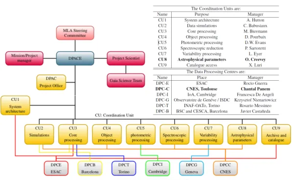
The Consortium is structured around specialized sub-units called Coordination Units (Fig. 2.4 and Table 2.1), each is responsible for a particular task of the overall Gaia data processing system. CUs develop the scientific algorithms and software, that later are run by one of the data processing centres (DPCs). These centres host the computing hardware and provide software engineering support to the CU, and each supports at least one CU.

(34)

2.2. Data Processing and Analysis Consortium 19

Figure 2.4: Coordinate Units separation in Gaia mission, more information can be found on the web-page http://www.mpia.de/gaia/about/cus

Figure 2.5: Component modules in Apsis and their interdependency. The module names are defined on the right panel. The arrows indicate a dependency on the output of the preceding module. The coloured bars underneath each module indicate which data it uses. Most of the modules additionally use the photometry and some also the Galactic coordinates. Credit:

(35)

The Coordination Units are:

Name Purpose Manager

CU1 System architecture A. Hutton

CU2 Data simulations C. Babusiaux

CU3 Core processing M. Biermann

CU4 Object processing D. Pourbaix

CU5 Photometric processing D.W. Evans

CU6 Spectroscopic reduction P. Sartoretti

CU7 Variability processing L. Eyer

CU8 Astrophysical parameters O. Creevey

CU9 Catalogue access X. Luri

The Data Processing Centres are:

Name Place Manager

DPC-E ESAC Rocio Guerra

DPC-C CNES, Toulouse Chantal Panem

DPC-I IoA, Cambridge Francesca De Angeli

DPC-G Observatoire de Genéve / ISDC Krzysztof Nienartowicz

DPC-T INAF-OATo, Torino Rosario Messineo

DPC-B BSC and CESCA, Barcelona Javier Castañeda

Table 2.1: The list of the wavelengths of adopted MgI and YII lines. Left column represents the core wavelengths for each line, and the used for the abundance estimation wavelength ranges are included in other two columns.

2.3 CU8 and GSP-Spec

The coordinate unit eight CU8 Astrophysical Parameters, is in charge of the classification and the parametrization of the observed targets (Bailer-Jones et al.,2013). Eleven modules of analysis compose the global CU8 astrophysical parameters inference system (APSIS, see Fig. 2.5). In particular, the working group General Stellar Parametrizer – Spectroscopy (GSP-Spec) is responsible for the main parametrization of the RVS spectra (Recio-Blanco et al.,

2016). To complement this GSP-Spec parametrization, other CU8 modules (Extended Stellar Parametrizer, ESP) will also estimate atmospheric parameters from RVS spectra of more specific types of stars as emission-line stars ELS), hot stars HS), cool stars (ESP-CS) and, ultra-cool stars (ESP-UCD) (Bailer-Jones et al.,2013). This thesis work has been partially developed in the framework of the CU8/GSP-Spec working group. In particular, the automatic algorithm of the determination of individual chemical abundances integrated in GSP-Spec has been optimized and tested (Chapter 4).

(36)

2.4. The Gaia data releases 21

2.4 The Gaia data releases

2.4.1 First data release DR1

Figure 2.6: The poster of IAUS 330, "As-trometry and Astrophysics in the Gaia sky". Graphic credit: A. Titarenko. Concept: Y. Beletsky & OCA Communication service. Gaia DR1 is based on observations

col-lected between the 25 July 2014 and the 16 September 2015, e.g. during the first 14 months of Gaia’s routine operational phase. Gaia DR1 was released on the 14th of September 2016. In this data release, positions (α, δ) and G-magnitudes for all sources (1 142 679 769 objects) with accept-able formal standard errors on positions are reported. The five-parameter astrometric solution – positions, parallaxes, and proper motions – for stars in common between the Tycho-2 Catalogue (Høg et al., 2000) and Gaia is contained (2,057,050 objects). This part of Gaia DR1 is called the Tycho-Gaia Astrometric Solution (TGAS, Micha-lik et al. (2015), Lindegren et al. (2016)), the first full-sky five parameters astromet-ric solution using Gaia data. Histoastromet-rically, the information from the HIPPARCOS cat-alog (Perryman et al. (1982), van Leeuwen

(2007)) – the Hundred Thousand Proper Motions HTPM (Mignard, 2009) project – was thought to be used as the source of the improved proper motions for the Gaia mission. The big difference in time, 24 years between HIPPARCOS and the Gaia mission, allowed to detect interesting objects, for example, long-period astrometric binaries. Unfortunately, HTPM has a number of limitations, that requires the use of additional "auxiliary" starsMichalik et al.

(2014). In this case, the full astrometric solution could be polluted by a potential bias, in-volved by these "auxiliary" stars. In the paper of Michalik et al. (2015) they have shown that the situation can be improved, if the full astrometric solution is solved using the Tycho-2 stars instead of "auxiliary" stars. Typical errors in parallax are 0.64 mas for 90% of all TGAS sources sources, including the subsets with a precision of 0.24 mas for 10% of the sources and 0.32 mas for 50% of the sources. Corresponding errors in proper motion are 0.72, 1.32 and 3.19 mas yr−1 respectively. The additional systematic parallax error is about 0.3 mas.

Limitations.

The initial Gaia DR1 is not a complete survey. In particular, the source list is incomplete at the bright part (G ≤ 7). All sources were treated as single stars without taking into account their radial velocities. Moreover, in dense areas of the sky (above some 400,000 stars per

(37)

square degree) the reported magnitude limit of Gaia DR1 may be brighter by up to several magnitudes. Finally, the sources that are close to bright objects are sometimes missing as well as high proper motion stars (µ >3.5 arcsec yr−1).

Contribution.

I have participated in the preparation of IAU Symposium 330, "Astrometry and Astrophysics in the Gaia sky", held in Nice in 2017. In particular, I created the graphic concept of Gaia and the grande coupole at OCA (Fig. 2.6). Lately, the concept was used for German postal-stamps as an advertisement of the Gaia mission.

2.4.2 Second data release DR2

Gaia DR2 data are based on observations collected between the 25th July 2014 and the 23th May 2016, covering a period of 22 months. It has been released the 25th April 2018.

The five-parameter astrometric solution – positions (α, δ), parallaxes, and proper motions – for more than 1.3 billion sources, with a limiting magnitude of G = 21 and a bright limit of G ∼ 3 are reported. In the Gaia DR2 parallaxes and proper motions are based on Gaia data only and do no longer depend on the Tycho-2 Catalogue. For an additional set of more than 361 million sources, a two-parameter astrometric solution is also reported. It includes the positions on the sky (α, δ) combined with the mean G magnitude.

Parallax uncertainties reach 0.04 milliarcsecond for sources at G < 15, 0.1 mas for sources with G = 17, and 0.7 mas at G = 20. The corresponding uncertainties in the re-spective proper motion components reach 0.06 mas yr−1(for G < 15 mag), 0.2 mas yr−1(for G = 17 mag) and 1.2 mas yr−1 (for G = 20 mag).

Median radial velocities for more than 7.2 million stars with a mean G magnitude between about 4 and 13 and an effective temperature in the range of about 3550 to 6900 K are reported. The overall precision of the radial velocities at the bright end reaches 200-300 m s−1 while at the faint end the total precision reaches 1.2 km s−1for a Tef f = 4750 K and 2.5 km s−1for a Tef f = 6500 K.

GBP and GRP magnitudes for more than 1.38 billion sources, with precisions varying from a few milli-mag at the bright (G < 13) end to around 200 milli-mag at G = 20 are reported. Additionally, a classification for more than 550,000 variable sources consisting of Cepheids, RR-Lyrae, Mira and Semi-Regular Candidates, High-Amplitude δ Scuti, BY Draconis candidates, SX Phoenicis Candidates and short time scale phenomena is reported.

The effective temperatures estimation is reported for more than 161 million sources brighter than 17th magnitude with effective temperatures in the range 3000 to 10 000 K. For a subset of about 87 million sources also the line-of-sight extinction AG and reddening E(from BP-RP instruments) are given. For part of this subset (around 76 million sources) the luminosity and radius estimations are available.

Limitations.

The Gaia DR2 catalogue is essentially complete between G = 12 and G = 17. Although the completeness at the bright end (G ≤ 7) has improved, it still has some problems with the

(38)

2.5. Summary 23

faint magnitude limit.

The completeness near bright sources and for high proper motion stars have significantly improved with respect to Gaia DR1. In dense areas of the sky (above some 400,000 stars per square degree) the magnitude limit of Gaia DR2 is now G = 18.

No radial velocity determination is available for objects identified as emission-line stars and detected double-lined spectroscopic binaries. Single-lined spectroscopic binaries have been treated as single stars and only a median radial velocity is provided.

The values of Teff, extinction AG, radius, and luminosity were determined only from the three broad-band photometric measurements and the parallax. A strong degeneracy between Teff and extinction/reddening when using the broad band photometry exists.

Contribution.

As a DPAC CU8 member, I am a co-author of 6 papers on Gaia DR2.Gaia Collaboration et al.

(2018b) is one of the main papers, consisting on the contents summary and survey properties. The other papers are performance verification articles: Gaia Collaboration et al.(2018a) is about observational Hertzsprung-Russell diagrams,Mignard et al.(2018) is dedicated to the celestial reference frame,Gaia Collaboration et al.(2018e) is about the observations of solar system objects,Gaia Collaboration et al.(2018d) mapping the Milky Way disk kinematics, and finally,Gaia Collaboration et al.(2018c) describes kinematics of globular clusters and dwarf galaxies around the Milky Way.

2.4.3 Future DR3+

As it was mentioned before, the next Gaia catalogue will be published at the end of 2020. This will be definitively the stellar catalogue that will play a central role for many varied fields of astronomy. It will contain the full astrometric solution (positions, distances and motions) and photometric data (brightness and color) for over one billion stars. As an extension, object classification and astrophysical parametrisation, together with BP/RP spectra and/or RVS spectra they are based on, will be released for spectroscopically and spectro-photometrically data. It will also include non-variable stars with available atmospheric-parameter estimates, variable stars, multiple stellar systems and exoplanet-hosting stars. For more than 150 million stars the radial velocities will be released.

The next Gaia data release DR3 will be first release of products for the CU8/GSP-Spec module of the DPAC APSIS pipeline.

2.5 Summary

This thesis is developed in the framework of the Gaia DPAC consortium, in particular to optimize the abundance estimation capabilities of the GSPspec module. In addition, the ar-rival of the first Gaia astrometric data has started the observational revolution of the Galactic Archaeology studies. In this thesis work the Gaia DR1 astrometric measurement were ex-ploited to study the possible use of a particular chemical abundance ratio [Y/Mg] as a stellar

(39)

age estimator. To this purpose complementary high-resolution spectroscopic data from the AMBRE project (Chapter 3) were used.

As shown in the Fig. 2.7, adapted fromGilmore(2012), the complementary use of Gaia and ground based spectroscopic data allows to explore the complete vision of the galactic stellar populations.

Figure 2.7: Diagrammatic representation of the outputs of the Gaia and AMBRE databases, showing how they are complementary. Adapted from: Gilmore et al.(2012)

(40)

Chapter 3

Building up the AMBRE-TGAS

catalogue

3.2 Procedures . . . . 26 3.2.1 Object identification: search radius . . . 27 3.2.2 Object identification: estimated photometric temperatures. . . 27 3.2.3 Object identification: comparison of object names . . . 27 3.2.4 Object identification: quality labels . . . 28 3.2.5 Additional flags for post-cross-match validation . . . 28

3.3 AMBRE HARPS . . . . 29

3.4 AMBRE UVES. . . . 33

3.5 AMBRE FEROS . . . . 36

3.6 Summarizing different instruments: the total AMBRE catalogue . . . . . 40

3.7 The AMBRE – TGAS catalogue . . . . 43

At the epoch of big spatial projects, such as Gaia, the ground-based observations are still playing an important role. In particular, high-resolution spectroscopic observations, covering a large wavelength domain, are important complement for Gaia data. Moreover, the huge amount of high-resolution spectroscopic data, collected from different ground-based instruments during the last years, is archived and available in open access. A clear example of this is the ESO archive advanced data products.In this thesis, the capabilities of the ESO archival data were exploited, analysing the AMBRE project (de Laverny et al., 2013). This huge amount of the data requires a homogeneous treatment, in order to extract from the results the highest precision level. In particular, this chapter is dedicated to the analysis of the stellar coordinates for the different ground-based spectroscopic data. Its goal is the improvement of the existing catalogue thanks to a homogeneous objects identification, capable to overcome the challenges of the complexity of a data base that is build up from archive data.

Stellar chemical clocks in the Gaia era

HAL Id: tel-01923867

https://tel.archives-ouvertes.fr/tel-01923867

Stellar chemical clocks in the Gaia era

Anastasia Titarenko

To cite this version:

Indicateurs chimiques d’âge stellaire

à l’ère de Gaia

Anastasia TITARENKO

Laboratoire J-L. Lagrange - Observatoire de la Côte d’Azur

Présentée en vue de l’obtention du grade de docteur

en Sciences de la Planète et de l’Univers

de l’Université Côte d’Azur

Thése dirigée par: Alejandra Recio-Blanco

Soutenue le: 21 Septembre 2018

M.

Carlos Abia

Professeur

Rapporteur

Mme.

Elisa Delgado Mena

Chercheur

Rapporteur

M.

Mathias Schultheis

Astronome

Président, Examinateur

Indicateurs chimiques d’âge stellaire

à l’ère de Gaia

Jury

Président du jury et Examinateur:

Rapporteurs:

Résumé

Abstract

Remerciements

Acknowledgements

Contents

Chapter 1

Introduction

Contents

1.1

Historical aspects and present day context

1.2

Stellar components of the Galaxy

1.2.1

The thin and the thick disks

1.3

Stellar Ages

1.3.1

Asteroseismology

1.3.2

Nuclear cosmochronology

1.3.3

Isochrone fitting methods

1.3.4

Indirect chemical proxies

1.4

Spectroscopy of stellar atmospheres

1.4.1

Continuous spectra

1.4.2

Spectral lines

1.5

The models of stellar atmospheres

Chapter 2

The Gaia mission as a new observational

era

Contents

2.1

Gaia instruments

2.1.1

Astrometry: ASTRO

2.1.2

Photometry: BP/RP

2.1.3

Spectroscopy: RVS

2.2

Data Processing and Analysis Consortium

2.3

CU8 and GSP-Spec