HAL Id: tel-00353827
https://tel.archives-ouvertes.fr/tel-00353827
Submitted on 16 Jan 2009HAL is a multi-disciplinary open access
archive for the deposit and dissemination of sci-entific research documents, whether they are pub-lished or not. The documents may come from teaching and research institutions in France or abroad, or from public or private research centers.
L’archive ouverte pluridisciplinaire HAL, est destinée au dépôt et à la diffusion de documents scientifiques de niveau recherche, publiés ou non, émanant des établissements d’enseignement et de recherche français ou étrangers, des laboratoires publics ou privés.
Geoffrey Decrouez
To cite this version:
Geoffrey Decrouez. Generation of multifractal signals with underlying branching structure. Signal and Image processing. Institut National Polytechnique de Grenoble - INPG; University of Melbourne, 2009. English. �tel-00353827�
No attribué par la bibliothèque
|
_
|_
|_
|_
|_
|_
|_
|_
|_
|_
| THESE EN COTUTELLE INTERNATIONALEpour obtenir le grade de
DOCTEUR DE L’Institut polytechnique de Grenoble et
de l’Université de Melbourne
Spécialité: Signal, Image, Parole, Télécommunications préparée au laboratoire GIPSA-lab, Département Images et Signaux dans le cadre de l’Ecole Doctorale Electronique Electrotechnique,
Automatique et Traitement du Signal
et au Département des Mathématiques et Statistiques de l’Université de Melbourne
présentée et soutenue publiquement par
Geoffrey DECROUEZ le 12 janvier 2009
GENERATION DE SIGNAUX MULTIFRACTALS POSSEDANT UNE STRUCTURE DE BRANCHEMENT SOUS-JACENTE
DIRECTEURS DE THESE:
Pierre-Olivier AMBLARD/Owen Dafydd JONES CO-DIRECTEURS DE THESE:
Jean-Marc BROSSIER/Konstantin BOROVKOV
JURY
M. Stéphane JAFFARD, Président
M. Patrice ABRY, Rapporteur
M. Benjamin Michael HAMBLY, Rapporteur
MM. Pierre-Olivier AMBLARD/Owen Dafydd JONES, Directeurs de thèse MM. Jean-Marc BROSSIER/Konstantin BOROVKOV, Co-encadrants
Firstly, I would like to thank my French and Australian supervisors and universities for making this PhD in cotutelle possible. Thanks Owen for your availability, at any-time. I enjoyed our discussions, and I greatly appreciate your help for making my arrival in Melbourne so easy. Thanks for your helpful suggestions for the writing of my thesis. It was a real pleasure working with you, always in a friendly environment. Thank you to my supervisor and mate Bidou for giving me so much freedom during my PhD, without it, this cotutelle program would have never happened. Also, it was good having you in Australia last year, our discussions on my work with Owen on this occasion were very helpful. Thank you Jean-Marc for the long conversations we had on the phone, for your availability, even when it was summer holidays in France. Your advice for the writing of this thesis was always very helpful.
I would like to thank everyone who has helped me directly or indirectly in the content of my thesis. In particular, thank you to Darryl Veitch for allocating some of your time to talk about my research. Thanks also to David Rolls for the many discussions we had. I would also like to express my gratitude to Patrice Abry for providing me with Matlab code, which has been very helpful for the numerical re-sults obtained in this thesis. Finally, thanks to Kostya Borovkov and Aihua Xia for being part of the committee for my confirmation talk at Melbourne University.
Then, I want to thank all my wonderful Australian friends who have helped me correct my English in this thesis. In particular, a big thank you to Tom Ballard, Ellie Button, Andrew Downes, Felix Ellet, Matthew Green, Paul Keeler, Heather Lons-dale, Rohan Malhotra, Anthony Mays, Jasper Montana, Michael Wheeler and Matt Zuparic for their suggestions. Cheers to my officemates, without them I wouldn’t know that the capital city of Lesotho is Maseru and I still couldn’t place Swaziland on a map. Thanks also to Andrew for reading part of my thesis while we spent hours and hours in Singapore waiting for passport controls to go to Malaysia. What a day. I also want to thank my friend Jasper for his understanding and his support throughout my thesis. Cheers to my great friend Prune for providing me a shelter and a mattress everytime I go back to Grenoble. Her place has become the most friendly squat in the whole city. I also want to give a big thank you to my parents, for making my exile at the other side of the world possible, but also for you support, and your wonderful help in all the horrible administrative tasks which makes this cotutelle possible. I promise I will go back to France . . . one day.
Last, but not least, I want give a warm thank you to Daniel Baudois for transmitting to me his passion for signal processing. Without you as a lecturer, I would probably not have pursued my studies in this area.
Acknowledgements 3
List of Symbols 9
1 Introduction 11
1.1 Fractals, multifractals and other oddities . . . 12
1.1.1 A first glimpse into self-similarity . . . 12
1.1.2 Various definitions of dimensions . . . 14
1.1.3 Iterated Function Systems (IFS) . . . 16
1.1.4 Brownian Motion and fBm . . . 18
1.1.5 Strict Self-Similarity . . . 20
1.1.6 H-SSSI processes . . . 20
1.1.7 Hölder regularity and fractal processes . . . 21
1.1.8 Multiplicative cascades . . . 21
1.1.9 Multifractal formalism . . . 25
1.2 Research work . . . 29
1.2.1 Galton-Watson Iterated Function Systems . . . 29
1.2.2 Multifractal Embedded Branching Processes . . . 30
2 Galton-Watson Iterated Function Systems 31 2.1 Self-similar sets and measures . . . 31
2.1.1 Contractive operators in metric spaces . . . 31
2.1.2 Complete space of compact sets . . . 32
2.1.3 Construction of self-similar sets . . . 33
2.2 Iterated Function Systems on functions . . . 34
2.2.1 Deterministic IFS . . . 34
2.2.2 Lp spaces . . . 35
2.2.3 Galton-Watson IFS . . . 38
2.3 Space of extended trees . . . 38
2.4 Existence and Uniqueness of a fixed point . . . 41
2.5 Properties of the fixed point . . . 44
2.5.1 Continuity of the sample paths . . . 46
2.5.2 Continuous dependency w.r.t. q . . . 46
2.5.3 Test for multifractality . . . 49
3 A multifractal embedded branching process 53
3.1 EBP and the crossing tree . . . 53
3.1.1 Construction of the Canonical Embedded Branching Process (CEBP). . . 53
3.1.2 Extension of the support of the CEBP . . . 60
3.2 From CEBP to MEBP . . . 64
3.2.1 The measure ν . . . 64
3.2.2 Existence and continuity of the MEBP . . . 65
3.2.3 Continuity of M . . . . 68
3.3 On-line simulation . . . 70
3.3.1 Markov representation . . . 70
3.3.1.1 Markov representation of CEBP . . . 70
3.3.1.2 Markov representation of MEBP . . . 72
3.3.2 On-line algorithm . . . 72
3.3.3 Efficiency . . . 79
3.4 Fractional Brownian Motion . . . 79
4 Multifractal formalism for CEBP and MEBP processes 89 4.1 Monofractals versus Multifractals . . . 89
4.2 The CEBP process . . . 91
4.3 Multifractal formalism for MEBP . . . 96
4.3.1 Multifractal formalism . . . 96
4.3.2 Discretization of the local Hölder exponent . . . 98
4.3.3 An upper bound for the spectrum of M . . . . 99
4.3.3.1 Coarse spectrum . . . 100
4.3.3.2 Deterministic coarse spectrum . . . 101
4.3.3.3 Large deviations . . . 102
4.3.3.4 Partition function τh . . . 104
4.3.3.5 Deterministic partition function Th . . . 107
4.3.3.6 Deterministic coarse spectrum of M . . . . 110
4.3.4 An upper bound for the spectrum of a subordinated Brownian motion. . . 115
4.4 Special points on the spectrum of ν . . . 120
4.4.1 The branching measure η . . . 120
4.4.2 The weighted branching measure ν . . . 121
5 Further work 125
Appendix A: The Legendre Transform 129
1.1 Fractal sets . . . 13
1.2 Construction of the deterministic binomial measure . . . 23
1.3 Partition function and Hausdorff spectrum of the deterministic bino-mial measure . . . 24
1.4 Wavelet Leaders. . . 27
2.1 Decomposition of the contractive operator T acting on Lp. . . 35
2.2 Fixed points of deterministic IFS . . . 36
2.3 Construction of Galton-Watson IFS . . . 39
2.4 Construction of the probability space of extended trees . . . 41
2.5 Fixed point and moments of a Galton-Watson IFS . . . 45
2.6 Estimation of the partition function of a fixed point of a Galton-Watson IFS . . . 50
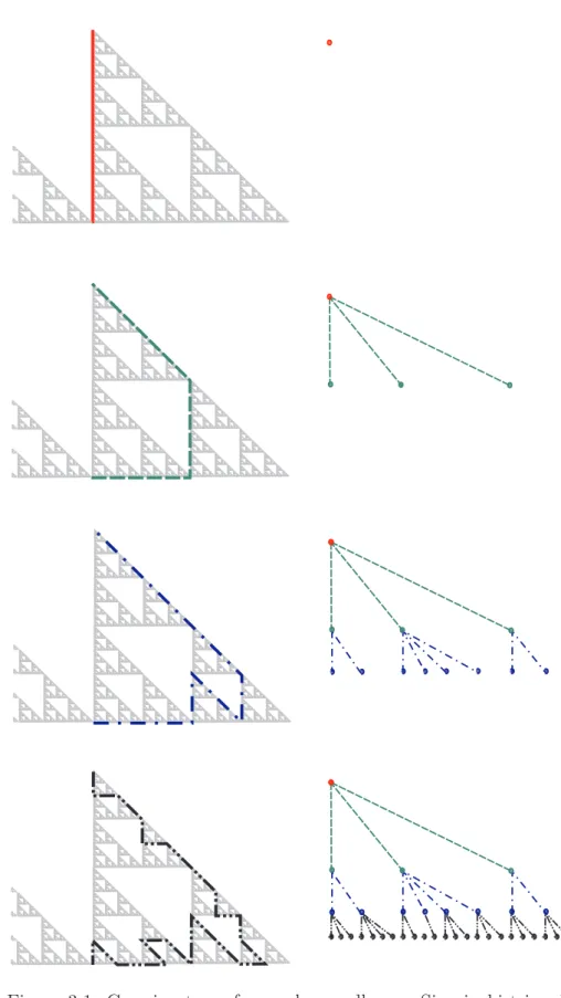
3.1 Crossing tree of a random walk on a Sierpinski triangle . . . 54
3.2 Crossing tree of a signal . . . 56
3.3 CEBP process, its crossing tree and crossing time durations. . . 61
3.4 Realisation of CEBP processes . . . 62
3.5 Cylinder sets and their mapping onto intervals of the real line . . . . 65
3.6 Relationships between the spaces of EBP, CEBP and MEBP processes. 68 3.7 Branching Random Walk . . . 69
3.8 Markov representation of CEBP processes. . . 71
3.9 Description of the on-line MEBP algorithm. . . 73
3.10 Realisations of a CEBP and MEBP processes . . . 80
3.11 Sketch of fBm simulated using the Chan-Wood algorithm . . . 82
3.12 Estimated offspring distribution of an fBm . . . 83
3.13 Estimation of the average crossing times of subcrossings for fBm and MEBP . . . 83
3.14 Marginal distribution, correlation function and partition function of an MEBP that imitates an fBm. . . 84
3.15 A realisation of an fBm generated using the Chan-Wood algorithm and a realisation of an MEBP process imitating an fBm . . . 87
4.1 Estimation of the partition function of CEBP processes . . . 95
4.2 Discretization of the Hölder exponent . . . 99
4.3 Intervals Ri . . . 111
4.4 Estimation of the partition function of M . . . 116 7
4.5 Estimation of the partition function of a subordinated Brownian motion119 5.1 Marginals of a time changed Brownian motion simulated using the
MEBP algorithm, and its correlation matrix. . . 127
5.2 Illustration of the Legendre transform. . . 131
5.3 Ensembles fractals . . . iv
5.4 Attracteur et moyennes d’un IFS de Galton-Watson . . . vii
5.5 Construction de l’arbre de branchement. . . x
5.6 Construction du processus CEBP. . . xi
5.7 Réalisations de processus CEBP . . . xiii
5.8 Réalisations de processus CEBP et MEBP . . . xv
5.9 fBm et processus MEBP. . . xvii
DH Hausdorff dimension . . . 15
D(h) Multifractal spectrum . . . .21
ξ(q) Legendre-Fenchel transform of D(h) . . . 26
dX(j, k) Wavelet coefficient of X at scale j and position k . . . 27
ζ1(q) Partition Function using wavelet coefficients . . . 27
LX(j, k) Wavelet leader of X at scale j and position k . . . 28
ζ2(q) Partition Function using wavelet leaders . . . 28
Lip(f) Lipschitz constant of a function f . . . 32
H(R2) Set of compact subset of R2 . . . .32
dH Hausdorff metric on H(R2) . . . 32
Lp(X) Space of p-integrable functions X → R . . . 34
dp Metric on Lp . . . 34
Lp Space of random p-integrable functions . . . .37
d∗p Metric on Lp . . . 37
̺j Random contractive maps . . . 38
rj Random contractive factor of ̺j . . . 38
φj Random function of two variables Lipschitz in its first variable . . . . 38
sj Random lipschitz constant of φj . . . 38
(K,K, κ) Probability space of extended Galton-Watson trees . . . .40
∅ Roof node of a tree . . . 41
Z∅ Number of branches rooted at ∅ . . . .41
i Node of a tree . . . 41
λp Contractive factor of Galton-Watson IFSs . . . 42
Tn k k-th level n passage time . . . .55
(Ω,F, P) Probability space of crossing trees with random weights . . . 55
Zn k Number of level (n − 1) subcrossings that make up the k-th level ncrossing . . . .55
p(x) Offspring distribution of a Galton-Watson tree . . . 55
pc|z(·) Orientation distribution . . . .57
|i| Length of i . . . 57
i|n Curtailment of i after n terms . . . 57
Υ Galton-Watson tree . . . 57
ΥGW n Generation n of Υ . . . 57
ZGW n Cardinal of ΥGWn . . . .57
µ Mean family size . . . .57
W∅ Limit of the martingale µ−nZnGW . . . 57
Υi Subset of Υ . . . 57
∂Υ Boundary of Υ . . . .57
ψ(i) Position of i within generation |i| . . . 57
Wi Limit of a martingale defined on Υi . . . 60
ρi Weight assigned to node i . . . .64
Wi Martingale limit attached to node i . . . 64
Ci Cylinder set . . . 65
ν Measure on ∂Υ . . . 65
Ri Interval constructed from Ci . . . 65
ζ Mapping of ν from ∂Υ to [0, W∅] . . . 66
hX(t) Local Hölder exponent of the process X at t . . . 90
Θa Set of points with local Hölder exponent a . . . 90
hM(t) Hölder exponent of M . . . 98
si ρi−Wi−+ ρiWi+ ρi+Wi+ . . . .98
f (a) Coarse spectrum of M . . . 100
N(n)(a, ǫ) Number of nodes on generation n with exponent in [a− ǫ, a + ǫ] . 100 F (a) Deterministic coarse spectrum of M . . . 101
τh(q) Partition function using h(t) . . . 105
˜ τh(q) τh(q)− 1 . . . 105
˜ τh∗(a) Legendre transform of ˜τh(q) . . . .105
Th(q) Deterministic partition function using h(t) . . . 108
˜ Th(q) Th(q)− 1 . . . 108
˜ T∗ h(a) Legendre transform of ˜Th(q) . . . 108
Sh n(q) . . . 108
Sh n(q) . . . 108
γn M(i) A discrete version of hM(t) . . . 110
Sγ n(q) . . . 110
Sγ n(q) . . . 110
τγ(q) Partition function using γ . . . 110
Tγ(q) Deterministic partition function using γ . . . 110
˜ τγ(q) τγ(q)− 1 . . . 110
˜ Tγ(q) Tγ(q)− 1 . . . 110
Introduction
"It is not necessary that you leave the house. Remain at your table and listen. Do not even listen, only wait. Do not even wait, be wholly still and alone. The world will present itself to you for its unmasking, it can do no other, in ecstasy it will writhe at your feet."
Franz Kafka Throughout the centuries, mathematicians have attached lots of credit to objects with nice properties, like spheres, lines, circles or differentiable curves and func-tions. Other mathematical objects were considered as "pathological", like irregular sets with no derivative almost everywhere. In a letter addressed to Emile Bernard in April 15th 1904, Paul Cézanne said: "Let me repeat what I told you when we were here: render nature with the cylinder, the sphere and the cone, arranged in perspective so that each side of an object or of a plane is directed towards a cen-tral point" [38]. For him, it was essential to learn how to paint "with reference to these simple shapes". Almost a century later, Mandelbrot claimed "clouds are not spheres, mountains are not cones, coastlines are not circle, and bark is not smooth, nor does lightning travel in straight line" [85]. The birth of the fractal geometry rests on Mandelbrot’s observations of the world. His merit was to put these observations together with irregular objects scientists were considering as purely mathematical objects, to notice their shared properties and unify them to create what he called a fractal geometry. The term fractal, as defined by Mandelbrot, comes from the Latin fractus meaning broken and refers to very irregular sets. The rapid development of fractal geometry was soon recognized in many areas of science, as witnessed by the exponential growth in the number of papers on fractals during the past 20 years.
In this chapter, I recall the concept of a ‘physical fractal’ and strict self-similarity on sets through different famous examples. This will lead us to see how this concept can be adapted to the context of processes, which is the main focus of my research work. Self-similar processes whose graphs have a non integer dimension can be obtained through simple recursive procedures. Fixed points of Iterated Functions Systems (IFS) are one of them and are briefly presented later. We also present the class of random self-similar processes through different examples, including Brownian mo-tion and fracmo-tional Brownian momo-tions. Then we introduce multifractal processes
and review a few methods to estimate their properties. Finally, I present a general outline of my doctoral research work.
1.1
Fractals, multifractals and other oddities
1.1.1
A first glimpse into self-similarity
Traditional geometry cannot describe very accurately irregular objects of our world, for example a coastline, a mountain or a tree. Before the birth of fractal geometry, complicated geometrical shapes could only be represented by a map or by their images. When looking at a map of scale 1 : 100, 000, is it possible to measure the length of a coastline? What becomes this length if we now look at a more detailed map of scale 1 : 10, 000? As we zoom in, bays appear, increasing the total length of the coast. When seen at different scales, the coastline appears similar in some sense. Likewise for a mountain; a detail of the edge of a mountain looks like the whole mountain. One aim of mathematics is to provide approximate models to describe these objects from the real world. We propose to review famous examples which incorporate the property of similarity of their geometrical shape at different scales of magnification.
Let us start exploring this mathematical world with the famous Cantor ternary set (1875), a subset of the real line which contains no intervals but has as many points as an interval. This set, categorized as pathological and called ‘monster’ by the mathematician Charles Hermitte, can be obtained through a recursive procedure. Begin with the interval C1 = [0, 1] and remove its middle third. At the first stage,
you obtain a set C2 which is the union of two intervals: C2 = [0, 1/3]∪ [2/3, 1].
Repeat the same procedure on the two smaller intervals. Keep going infinitely many times. The limit set, C =TnCn is the Cantor ternary set, an uncountable set with
zero Lebesgue measure. Parts of C look like the original set C, up to a scaling factor. The journey continues with the Sierpinski gasket constructed by the Polish math-ematician W. Sierpinski. The idea is similar: start with a single region and remove parts of its interior. Let the initial set be a triangle S0 together with its interior.
Then, connect the midpoints of the sides with line segments and remove the inte-rior of the small middle triangular region. At the first stage, three smaller triangles replace the initial one. Call this set S1. Repeat the same procedure to the three
smaller triangles and continue infinitely many times. The limit set S = TnSn is the
Sierpinski triangle. An approximation of S is presented in the left upper corner of Figure 1.1, together with other limit sets obtained via similar recursive procedures. The sets are obtained with Matlab code that I have re-implented to produce them. The Sierpinski triangle possesses a similar property as the Cantor ternary set: each of the smaller triangles is an exact replica of S. Many other such examples exist, such as the Von Koch curve (a compact curve with infinite length), the Monger sponge, the Sierpinski carpet, to name but a few. In general, a figure or set which can be decomposed into parts which are exact replicas of the whole is called discrete strict self-similar.
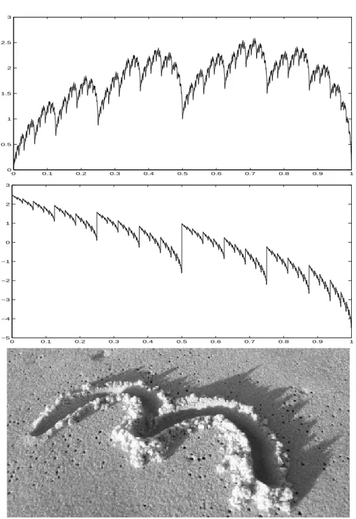
0 0.1 0.2 0.3 0.4 0.5 0.6 0.7 0.8 0.9 1 0 0.1 0.2 0.3 0.4 0.5 0.6 0.7 0.8 0.9 1 −5 −4 −3 −2 −1 0 1 2 3 4 5 −2 0 2 4 6 8 10 12 −6 −4 −2 0 2 4 6 −2 0 2 4 6 8 10 12 −8 −6 −4 −2 0 2 4 6 8 10 −2 0 2 4 6 8 10 12
Let us emphasize the major difference between fractals encountered in mathemat-ics, for which self-similarity occurs at all scales of magnification, and self-similar objects found in nature, called ‘physical fractals’, for which this self-similarity holds only for a range of scales. When looking at a coastline, for example, one cannot zoom indefinitely but only up to the atomic level. Mathematical fractals have played an important role in synthetic imagery and graphics [18] and have touched all branches of science. Applications range from biology (plant trees, bronchial trees, blood cir-culation systems) to network traffic [2], from art (in decoration, architecture, [108]) to pure mathematics.
1.1.2
Various definitions of dimensions
The next questions that come to mind are how to measure the irregularity of a set or a curve and how ‘big’ is a fractal set? Are the fractals presented in Figure 1.1 similar in some way? Also, we have not yet given an accurate definition of a fractal, other than the fact that it is an irregular set. Is it possible to give a more precise definition? A possible answer to these questions is related to the concept of dimension, which gives a good quantitative measure of how much a set or curve fills the space. The definition of dimension is not unique and throughout the history of mathematics, many definitions have been given. For example, the Euclidean dimension DE is the
number of coordinates needed to address the object. The topological dimension DT
requires coverings of the object. A covering is by definition a collection of open sets in a topological space X whose union contains the object. We also define a refinement of a cover C of X as a new cover C′ such that each set in C′ is contained
in some set in C. Then, an object A has topological dimension DT if every covering
C of A possesses a refinement C′ in which every point of A belongs to at most D T+ 1
sets in C′, where D
T is the smallest such integer. For example, as illustrated below,
a set of points distributed in the plane have DT = 0 and DE = 2. A smooth curve
in the plane has DT = 1 and DE = 2.
When dealing with irregular objects, other definitions of dimensions have to be used to compare them. These dimensions are referred to as fractional dimensions since they can take non integer values. The Hausdorff dimension DH of a set is a
central notion in fractal geometry. Fractional dimensions first appeared in 1919 with mathematician Felix Hausdorff but had to wait until the works of Mandelbrot to be related in a systematic way to fractals. Other fractional (or fractal) dimensions are the box counting and packing dimensions.
Hausdorff dimension. The Hausdorff dimension of a set is defined from its Hausdorff measure. To motivate the definition of the Hausdorff measure, we address the following question: given a curve c ⊂ R2, how do we measure its length? We
want some measure theory notion, independent of the properties of the curve, such as its differentiability. The idea is once again to cover c with balls Bj. Denote by
|Bj| the diameter of Bj. Then, an approximation of the length L(c) of c is P|Bj|.
However, the covering can have poorly placed balls or extra balls not needed to cover c. A better approximation of the length is then to take the infimum over all possible coverings: L(c)≈ infnX|Bj| | c ⊆ [ Bj o .
A second problem arises. A ball can do too well because it is too large: the sum is therefore too small because the balls do not follow the contours of the curve. Therefore, we approximate the length of c as the sum of the diameter of a ‘good’ covering of c, in the limit where the diameter of the balls tends to 0. Formally, fix δ > 0 and A⊂ Rp, then the previous discussion motivates us to define
Hnδ(A) = inf ( ∞ X j=1 |Bj|n | A ⊆ ∞ [ j=1 Bj, |Bj| 6 δ ) .
In the previous definition, we raise |Bj| to the power of n by analogy with covering
sets with balls in Rn. Since the infimum is made over a smaller number of possible
coverings as δ decreases, Hn
δ(A) increases and it is legitimate to consider the limit
as δ → 0:
Hn(A) = lim δ→0+H
n δ(A).
Hn(A) is the Hausdorff measure of A. In fact, one can show that as n increases
Hn(A) jumps from∞ to 0, and that there is at most one s with 0 < Hs(A) <∞. It
is always possible to define the biggest n for which Hn(A) is infinite, or equivalently
the smallest n such that Hn(A) = 0. This particular value of n is the Hausdorff
dimension of A:
DH(A) = sup{n | Hn(A) =∞} = inf {n | Hn(A) = 0} .
The corresponding Hausdorff measure of A is however not necessarily finite. In general, DH > DT. In fact, one cannot give a precise definition of a fractal, but
Falconer in [44] notices that most fractal sets K share the following properties: 1. K has details/irregularities at all scales.
2. K cannot be described using equations from classical geometry. 3. K is approximately, strictly or statistically self-similar.
4. The ‘fractal’ dimension of K is usually strictly greater than its topological dimension.
5. K can be constructed most of the time in a simple way, perhaps recursively. Box-counting dimension. Hausdorff dimension cannot be calculated directly in practice due to the infimum encountered in the definition. To this end, more
tractable definitions are needed. Box counting dimension dates back to the 1930’s and is also known as Kolmogorov entropy, entropy dimension, or capacity dimension. Its widespread use is due mainly to its ease of calculation. The idea is to cover the object A with sets of diameter r. Call Nr the number of such sets needed to cover
A. The box dimension is then
DB(A) = lim r→0
log Nr
− log r
if the limit converges (otherwise replace lim by lim inf or lim sup, respectively the lower and upper box counting dimensions). The box dimension is therefore the power law behaviour of the measurement of the object at scale r. The number of sets that can cover A is of order r−DB(A). The previous definition remains the same
if for Nr we consider the smallest number of cubes of diameter r that can cover
A [44], hence the name box counting dimension. To obtain an estimate of DB(A),
it suffices to plot log Nr versus log r. The slope of a linear interpolation gives an
estimation of DB(A).
For sufficiently smooth objects like a straight line, it is possible to have equality among the various definitions of dimension. However, in general this does not hold and DE >DB >DH>DT. We now review a recursive procedure to create sets for
which DE > DH.
1.1.3
Iterated Function Systems (IFS)
IFS are a simple way to generate fractal objects. Hutchinson pioneered the theory of non random self-similar fractal sets and measures via contracting mapping methods in his early work in 1981 [60]. He also introduced the notion of scaling operators. The terminology Iterated Function Systems appeared later on with the works of Barnsley and Demko [15].
The idea of an IFS is to recursively apply a set of contractive operators on a given set. A contraction ω : Rd→ Rd is a mapping for which there exists a c ∈ (0, 1) such
that ∀(x, y), |ω(x) − ω(y)| 6 c|x − y|. c is called the contraction factor of ω. An IFS consists of a collection of contractions {ω1, . . . , ωM} with M > 2, with contraction
factor c1, . . . , cM. Let H(R2) be the set of compact sets of R2 and define the operator
W by: W (A) = M [ i=1 ωi(A)
for all A ∈ H(R2). Then W is contractive with contraction factor c = max(c
i). One
can prove the existence and uniqueness of an attractor A∗ or fixed point of a given
IFS under mild conditions. A∗ satisfies
A∗ =
M
[
i=1
ωi(A∗) = W (A∗). (1.1)
The IFS is said to satisfy the open set condition if there exists a non empty open set O ⊆ Rn such that ∪ω
open set condition is strong enough to ensure good mathematical results (existence of a fixed point, properties of the fixed point, derivation of its Hausdorff dimension, etc.) but sufficiently weak to include a large number of examples. Under the open set condition, one can show that the Hausdorff dimension s = DH(A) of the attractor
A of the IFS satisfies [93]
M
X
i=1
csi = 1. (1.2)
We have already encountered two attractors of IFS in this introduction. The Cantor ternary set C is the fixed point of an IFS with two maps ω1(x) = x/3 and ω2(x) =
x/3 + 2/3 and satisfies C = ω1(C)∪ ω2(C). From Equation (1.2), it follows that
the Hausdorff dimension of C is log 2/ log 3. The Sierpinski triangle is also the fixed point of an IFS, consisting of 3 similarities of ratio 1/2. Its Hausdorff dimension is log 3/ log 2.
IFS received a great deal of interest in data compression. The target image is represented by the attractor of an IFS. The difficulty of the method is to obtain a set of contractive maps that approximate correctly the target image. When successful, the advantage is an enormous compression of information to encode the image.
Fractals encountered so far are all deterministic (IFS considered have non-random contraction mappings) and are strictly self-similar. It is possible to randomize the construction of fractals to break the strict self-similarity. The motivation to do so is that ‘physical’ fractals are statistically self-similar. In other words, when zooming in on a natural fractal, the detail has the same properties as the whole object without being exactly the same. Random fractals can also be easily obtained via random IFS when considering random maps ωi. Results on fractal sets have been adapted
to the study of random self-similar measures and functions. My research works were partly focused on IFS acting over the space of functions to produce self-similar random processes. The method used was based on previous results from Hutchin-son and Rüschendorff [63] and generalized one of their results on the existence and uniqueness of the attractor of an IFS, when allowing more randomness in the model. Sets encountered so far possess no characteristic space scale. To characterize them and give them a dimension, we had to look at the construction procedure and to understand how scales interact with each other. Motivated by this observation, we want a process exhibiting scale invariance not to have a characteristic time or scale, so that the whole signal or parts of it cannot be distinguished. One cannot use traditional techniques to study these processes. Instead, it is relevant to understand how properties of the process are related across scales. Dimension is one way of thinking about fractals, the other paradigm is scaling, better suited to signals. To illustrate this notion, we consider two famous processes as introductory examples: the Brownian motion and the fractional Brownian motion. Then, we discuss the notion of strict self-similarity and introduce models with a richer structure. In this thesis, a random function X(t) will be called either process or signal. The first term is more widely used among mathematicians while the second term is more common in the signal processing community.
1.1.4
Brownian Motion and fBm
Brownian motion B(t) was first observed by botanist Robert Brown in 1828 as he noticed the very irregular movement of pollen suspended in water [28]. The origin of the motion remained however unexplained and we had to wait until the works of Bachelier in stock price fluctuations in 1900 [11] and Einstein in 1905 [39] to obtain an explanation of the motion. Einstein predicted the motion of a sufficiently small particle caused by the random bombardment of the molecules of the liquid: the random number of collisions on the particle by molecules coming from different directions, with different strength, would cause an irregular motion of the particle. It turned out that the model gave a good description of the motion observed by Brown. A rigorous mathematical treatment of Brownian motion was given by Nor-bert Wiener in 1923. Applications of Brownian motion are in fact far beyond the study of microscopic particles floating in water. Its applications include modelling stock prices or thermal noise in electric circuits, but cover also random perturba-tions in many branches of science like physics, biology or economy. But Brownian motion has also played a major role in understanding fractals and self-similar pro-cesses. It can be constructed as a limit random walk in the plane or space. Limits of random walks on a Sierpinski gasket were also studied by Barlow and Perkins in 1988 [13]. They proposed to associate a branching process with the random walk (details about its construction are postponed to Chapter 3). This association was the primary motivation of the definition of Embedded Branching Processes (EBP) introduced by Jones in 2004 [69]. Part of my doctoral works consisted in extending EBP to a wider class of processes that we called Multifractal Embedded Branching Processes or MEBP.
Let us go back to the properties of B(t). Provided B(0) = 0, it can be shown that the Brownian motion is the only process satisfying the following 3 properties
1. For all τ > 0, the increment process ∆Bτ(t) = B(t + τ )− B(t) is Gaussian and
stationary.
2. For t1 6t2 6t3 6t4, increments B(t4)− B(t3) and B(t2)− B(t1) are
indepen-dent.
3. B(t) is continuous.
B(t) is the only Gaussian process with stationary and independent increments. B(t) and ∆Bτ(t) satisfy an interesting scaling law:
B(ct) = cd 1/2B(t) (1.3)
∆Bτ(ct) d
= c1/2∆Bτ(t) (1.4)
for all c > 0. Here = denotes equality in distribution. Relation (1.3) suggests thatd the sample paths of Brownian motion cannot be distinguished from a rescaled ver-sion, by dilating the time axis by a factor c and the amplitude axis by a factor c1/2:
there is no reference scale of time. Furthermore, the Hausdorff and box dimensions of its graph are non integer and equal 1.5 almost surely. This observation builds a first bridge between the notions of scaling law and fractal dimensions.
For modelling purposes, Brownian motion suffers from its simplicity. It is unlikely to be able to model all random processes with a graph whose dimension is 1.5, or equivalently, whose scaling exponent is fixed to 1/2. To obtain more general models, at least one of the 3 properties given above need to be relaxed. We can drop for example either the independence of increments, leading to the fractional Brownian motion (fBm) or the finite variance of increments to obtain the class of α-stable Lévy processes. fBm BH(t) was introduced by Mandelbrot and Van Ness in 1968
[89] as a moving average of dB(t), where past increments are convoluted by the kernel (t − s)H−1/2, for 0 < H < 1. BH(0) = 0 BH(t) = 1 Γ(H + 1/2) 0 Z −∞ ¡ |t − s|H−1/2− (−s)H−1/2¢dB(s) + t Z 0 |t − s|H−1/2dB(s) . In fact, fBm has the following properties
1. BH is continuous and BH(0) = 0.
2. BH(t + τ )− BH(t) is normally distributed with mean 0 and variance τ2H.
3. BH has stationary increments.
For H = 1/2, fBm reduces to Brownian motion. Under the assumption of finite variance, the covariance structure of fBm is fixed
EBH(t)BH(s) = E|BH(1)|
2
2 (|t|
2H+|s|2H− |t − s|2H).
A similar expression holds for increments of fBm (which are called fractional Gaus-sian noise (fGn)). The study of fGn can inform us about the behaviour of fBm. When 1/2 < H < 1, fGn is positively correlated and the correlation function is not integrable (it decreases as the power law τ2H−2). We are in presence of long-range
dependence (LRD) or long memory [20]. These notions can be compared with more classical processes with exponential decay of their covariance function, like ARMA processes.
One can show that fBm with parameter H has Hausdorff and box dimensions 2−H almost surely. BH(t) and its increments ∆BH,τ(t) := BH(t + τ )− BH(t) satisfy a
similar scaling law to (1.3)
BH(ct) d = cHBH(t) (1.5) ∆BH,τ(ct) d = cH∆BH,τ(t). (1.6)
The behaviour and properties of fBm can be fully derived through its only param-eter H. This simplicity is convenient for modelling but is also a drawback since fBm is too simple for many real world problems. It is unlikely that a whole range of scale invariant signals can be modeled by a class of processes with a single parameter. There exists other processes which generalise the Brownian motion. Stochastic dif-ferential equations are really the first extension to include a wider class of random processes.
1.1.5
Strict Self-Similarity
Relations (1.3) and (1.5) can be unified in the fundamental notion of self-similarity. A process X is said to be self-similar with index H if and only if a change of the time scale is equivalent to a change in the state space scale
∀c > 0 {X(ct), t ∈ R}f dd= {cHX(t), t∈ R}. (1.7)
Equality (1.7) holds in the sense of finite dimensional distributions (f dd= ), that is for any d > 1, t1, . . . , td,
(X(ct1), . . . , X(ctd))= (cd HX(t1), . . . , cHX(td)).
A process satisfying (1.7) was originally called semi-stable by Lamperti in 1962 [77]. Mandelbrot used the term self-similar 20 years later [85]. It follows immediately from this definition that for all t > 0, the moments of X behave as a power law
E|X(t)|q= E|X(1)|q|t|qH (1.8)
for all q such that E|X(t)|q is finite. Relation (1.8) shows that self-similar signals are
non-stationary. There exists however a relation between stationary and self-similar processes, given by Lamperti’s theorem [77].
1.1.6
H-SSSI processes
One usually restricts the class of self-similar processes to one of self-similar processes with stationary increments (SSSI processes) as they are more convenient to work with since their increments satisfy Ya(t) := X(t + a)− X(t)= X(a)d − X(0). If one
assumes finite variance, then the covariance structure of X is constrained to satisfy EX(t)X(s) = 1
2[|t|
2H+|s|2H − |t − s|2H]E|X(1)|2.
For the covariance function to be definite non-negative, it follows that the range of possible values of H is (0, 1]. The unique H-SSSI Gaussian process is the fractional Brownian motion introduced above and is the most widely used to model phenomena possessing scale invariance properties. Also, the self-similarity is transmitted to Ya:
E|Ya(t)|q= E|X(1)|q|a|qH. (1.9) We have already encountered this situation for fBm, where both the process and its (stationary) increments are self-similar. Note that in (1.8) and (1.9), the exponent is linear with q.
1.1.7
Hölder regularity and fractal processes
The concept of local Hölder regularity is closely related to the notion of self-similarity. Self-similar processes have parts (details) which are statistically similar to the whole. Zooming in on a detail of the process helps us learn about its the local fluctuations. Information about these local fluctuations can be made precise with the definition of the Hölder exponent of a process X(t) at a specific time t = t0. It compares
X(t0) with a polynomial Pt0(t). The process X is said to belong to C
h(t0)
t0 if there is
a polynomial Pt0 of degree at most equal to the integer part of h(t0) such that
|X(t) − Pt0(t)| 6 K|t − t0|
h(t0)
in a neighborhood of t0. The largest value H of h(t0) such that X ∈ Cth(t0 0) is the
Hölder exponent of X at t = t0. Alternatively, one says that the Hölder regularity of
X at t = t0 is H. Fractional Brownian motion BH(t) with self-similarity parameter
H (see Equation 1.9) has a fixed local Hölder exponent equal to H for all t. It follows that almost surely, for all t, |BH(t + δ)− BH(t)| is bounded above by KδH, for some
finite constant K. We refer to processes with a constant Hölder exponent along their sample paths as monofractals. It is possible to consider a more general class of processes for which the Hölder exponent varies smoothly and deterministically with time. These processes are called multifractional. The major drawback is once again the lack of flexibility since the Hölder exponent is the same at a given time for all realisations of the process. In network traffic applications, the rich structure of the data does not allow multifractional processes as good models [1]. Instead, it is interesting to consider the case when h(t) varies in an erratic way. The name multifractal was given to such processes, in opposition to monofractals with a single Hölder exponent. Due to the highly irregularity of h(t), it is not realistic to describe the fluctuations of multifractal processes in terms of the evolution of h with time. Instead, we depict the process by means of its multifractal spectrum D(h), a global description of its local fluctuations. D(h) is defined as the Hausdorff dimension of the set of points with a given Hölder regularity h. For monofractal processes, D(h) degenerates to a single point at h = H, D(H) = 1 and generally the convention is to set D(h) = −∞ for h 6= H.
1.1.8
Multiplicative cascades
The oldest and best known multifractal processes are the multiplicative cascades introduced by Mandelbrot in the context of intermittent turbulence in 1974 [84]. We review the construction of the deterministic binomial measure µ, indicate some generalizations and give results about their local behaviour.
Deterministic example. Let the support of µ be the real interval [0, 1). The idea is to allocate a mass or probability to each subinterval of [0, 1) of the form
In,k = h k 2n, k + 1 2n ´
as the intersection of all In,k for which t ∈ In,k
{t} = \
n>0
t∈In,k
In,k.
The binomial measure is constructed as the limit of a sequence of measures {µn}. Let
µ0([0, 1)) = 1. Start by splitting [0, 1) into two subintervals of equal length [0, 1/2)
and [1/2, 1). Allocate a mass m0 to [0, 1/2) and m1 to [1/2, 1), with m0+ m1 = 1,
µ1([0, 1/2)) = m0 µ1([1/2, 1)) = m1.
At stage n = 2, we divide each [0, 1/2) and [1/2, 1) into two subintervals of equal length to obtain intervals [0, 1/4), [1/4, 1/2), [1/2, 3/4) and [3/4, 1). [0, 1/4) receives a fraction m0 of the mass of [0, 1/2) and [1/4, 1/2) a fraction m1 of the mass of
[0, 1/2). Thus
µ2([0, 1/4)) = m20 µ2([1/4, 1/2)) = m0m1
µ2([1/2, 3/4)) = m1m0 µ2([3/4, 1)) = m21.
The figure below illustrates the binary branching structure associated with this construction
m0 m1
m m0 1 m m1 0 m m1 1
m m0 0
At stage n, the initial mass m0+ m1 = 1 is distributed among 2n dyadic intervals,
which defines a measure µn, piecewise uniform. Consider the dyadic expansion of t
t =
n
X
i=1
ξi2−i
for ξi ∈ {0, 1}. Let N = Pni=1ξi be the number of ones among the first n binary
digits of t, then, if t ∈ In,k,
µn(In,k) = mn−N0 mN1 .
Since for all m > n, µm(In,k) = µn(In,k), we may define the binomial measure µ to
be the limit of the sequence {µn} such that µ(In,k) = µn(In,k). Since µ([0, 1)) = 1
and µ is positive, the limit is well defined since (µn) is an increasing sequence,
bounded above. The construction of µ can be extended to all half-open subintervals [a, b) of [0, 1). By Carathéodory’s extension theorem, we can uniquely extend µ to
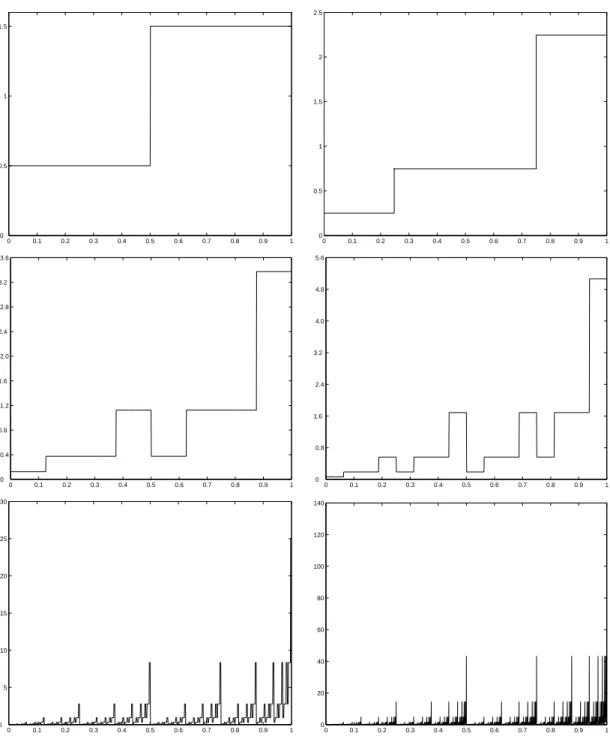
0 0.1 0.2 0.3 0.4 0.5 0.6 0.7 0.8 0.9 1 0 0.5 1 1.5 0 0.1 0.2 0.3 0.4 0.5 0.6 0.7 0.8 0.9 1 0 0.5 1 1.5 2 2.5 0 0.1 0.2 0.3 0.4 0.5 0.6 0.7 0.8 0.9 1 0 0.4 0.8 1.2 1.6 2.0 2.4 2.8 3.2 3.6 0 0.1 0.2 0.3 0.4 0.5 0.6 0.7 0.8 0.9 1 0 0.8 1.6 2.4 3.2 4.0 4.8 5.6 0 0.1 0.2 0.3 0.4 0.5 0.6 0.7 0.8 0.9 1 0 5 10 15 20 25 30 0 0.1 0.2 0.3 0.4 0.5 0.6 0.7 0.8 0.9 1 0 20 40 60 80 100 120 140
Figure 1.2: Construction of the deterministic binomial measure ν. From top to bottom, left to right, construction of the measure after 1, 2, 3, 4, 8 and
12 iterations, for m0 = 1/4 and m1 = 3/4. The measure is renormalized so that
R
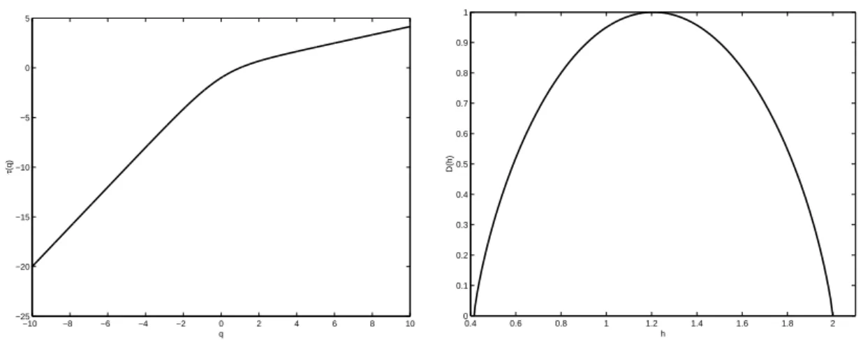
−10 −8 −6 −4 −2 0 2 4 6 8 10 −25 −20 −15 −10 −5 0 5 q τ (q) 0.4 0.6 0.8 1 1.2 1.4 1.6 1.8 2 0 0.1 0.2 0.3 0.4 0.5 0.6 0.7 0.8 0.9 1 h D(h)
Figure 1.3: Binomial cascade: partition function τ (q) and Hausdorff spectrum D(h)
when m0 = 0.25 and m1 = 0.75.
the σ-algebra generated by the dyadic intervals of [0, 1). The first few steps of the construction of µ with m0 = 1/4 and m1 = 3/4 are illustrated in Figure 1.2.
The binomial measure is by construction very irregular and possesses no density. We are generally interested in the process X(t) = R0tdµ. X(t) is multifractal unless m0 = m1 = 1/2 and its multifractal spectrum (defined at the end of the previous
section) is given by the Legendre-Fenchel (LF) transform of a so-called partition function τ (q) D(h) = inf q (qh− τ(q)) (1.10) where τ (q) is given by τ (q) =− log2(mq0+ m q 1). (1.11)
A review of the Legendre-Fenchel transform is given in Appendix A. As illustrated in Figure 1.3, the spectrum of the binomial measure with m0 = 0.25 and m1 = 0.75 is
concave. In fact, the concave ∩-shape of the spectrum of X is typical of multiplicative cascades. All results and observations about the multifractal spectrum in this section can be found in [102].
The dyadic deterministic construction can be easily generalized by splitting [0, 1) into b > 2 subintervals of equal length, each receiving a mass m0, . . . , mb−1 > 0,
P
kmk = 1. To this construction, we can associate a deterministic b-ary construction
tree, whose branches are equipped with the non-random weights m0, . . . , mb−1. The
spectrum of the integral of the limit measure is then the LF transform of the partition function τ (q) =− logb(m q 0+ . . . + m q b−1). (1.12)
Random example. The procedure can be randomized by allocating a random mass to each subinterval at each iteration. Dyadic intervals In,k therefore receive a
random mass
µ(In,k) = Mn,k(n). . . M1,k(1).
We usually make the following assumption about the random weights, for the random binary cascade:
• Conservation of the mass in the mean: E(M(n+1) n,2k + M (n+1) n,2k+1) = 1 • Mn,k(n)= Md 0 if k is even and Mn,k(n) d = M1 if k is odd.
where= denotes equality in distribution. Products of multipliers can be very smalld and despite the conservation in the mean, the total mass distributed over the interval [0, 1) may degenerate in some cases. However, under further conditions on the multipliers, one can show Eµ([0, 1)) = 1. The Hausdorff spectrum of the integral of the random binomial measure is then the LF transform of
τ (q) =− log2E(M0q+ M1q). (1.13)
The generalization of the construction of the random measure by splitting [0, 1) into b > 2 subintervals of equal length yields the partition function τ (q) =− log2E(M
q 0+
. . . Mb−1q ). Many other random cascades can be contemplated. In Chapter 3, we de-rive an upper bound for the Hausdorff spectrum of a new process defined as the integral of a measure obtained from a cascade construction on a random tree. The novelty is the way we define an embedding from the boundary of the random tree to intervals of the real line, which differs from previously proposed random partitions, for example [100].
1.1.9
Multifractal formalism
For estimation, detection or classification purposes in signal processing, it is impor-tant to be able to estimate the spectrum D(h) of a signal. It is a way to distinguish a monofractal process from a multifractal process for example. In practice, we are facing a double problem. Firstly, locating all points of the process with a given Hölder regularity is not feasible due to the finite precision of the data. Secondly, as discussed before, the difficulty in estimating the Hausdorff dimension of a given set due to the presence of the infimum in its definition. Alternative methods of estimations were sought, and gave birth to what is known as the multifractal for-malism. By multifractal formalism we mean a formalism where we calculate the Legendre-Fenchel transform (see Appendix A) of a partition function, which gener-ally provides an upper bound for the multifractal spectrum. When this upper bound is the multifractal spectrum, we will say that the multifractal formalism holds.
Multifractal formalism is associated with the study of the moments of multiresolu-tion quantities TX(a, t), obtained from a comparison of the original process with a
reference pattern ψ(t) dilated and located at different positions [3, 7] TX(a, t) =< X, ψa,t >=|a|−1
Z
X(u)ψ((u− t)/a)du (1.14)
where ψa,t(u) = |a|−1ψ((u− t)/a). In previous sections, we considered increments
of SSSI processes. It is easy to see that increments are the result of the comparison of the original process X(t) with ψ(t) = δ(t + τ0)− δ(t), where δ(t) is the Dirac
by considering techniques based on wavelets coefficients. The study of E|TX(a, t)|q
is in practice replaced by time averages, under the assumption that the {TX(a, tk)}k
form a stationary sequence, for some partition tk, k ∈ Z. Then, a process X is said
to possess scaling properties if the time averages of TX(a, tk) follow a power law
behaviour with respect to a 1 na na X k=1 |TX(a, tk)|q ≃ Cq|a|ζ(q)
where na is the number of TX(a, tk) available at scale a. ζ(q) is called the partition
function. Usually, this behaviour is valid only for a limited range of finite scales and a limited range of q. It is worth mentioning that the power law behaviour of time averages may differ from the power law behaviour (if it exists) of ensemble averages. To illustrate this counterintuitive fact, it has has been demonstrated that Compound Poisson Motions [19] have stationary increments which satisfy [32]
E|TX(a, t)|q≃ Cq|a|λ(q)
in the limit as a → 0. This expression holds for a finite range of q ∈ (0, q+
c) where
q+
c is the largest q such that E|TX(a, t)|q is finite. Although it is tempting to believe
that ζ(q) and λ(q) agree on (0, q+
c), it is now acknowledged that equality holds only
for a smaller range of q values [92, 98].
The choice of TX(a, t) plays a central role for the estimation of the partition
func-tion. Multiresolution quantities based on a wavelet decomposition of the process are the most powerful tool to date [1, 3, 7, 8, 66], since they allow the study of the signal at different scales and positions. We introduce ξ(q), the LF transform of D(h),
ξ(q) = 1 + inf
h (qh− D(h)).
In the next section we recall relations between ξ(q) and ζ(q), for two expressions of TX(a, t).
Wavelet based estimators. The discrete wavelet transform is a time/scale representation of a signal X(t) using a multiresolution analysis, decomposing a signal into two parts: approximations and details. Approximations are obtained as the result of projections of the signal onto a low frequency function φ0, called the scaling
function [82, 91]. This operation realizes a low-pass filter and retains the slow variations of the signal. Details are obtained after comparison of the signal with a high frequency function called the mother wavelet ψ0. This projection performs a
high-pass filter of the signal and only keeps its fast variations. To reconstruct the signal from its projections on ψ0 and φ0, ψ0 must satisfy the admissibility condition
[50] Z
R
ψ0(t)dt = 0.
A wavelet is described by the number N of its vanishing moments Z
j
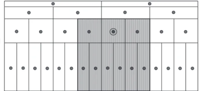
Figure 1.4: The Wavelet leader LX(j, k) in black circle is defined as the maximum
of all detail coefficients dX(·, ·) (black dots) over 3λj,k represented in a shaded area
in the picture.
Let ψj,k(t) = 2−j/2ψ0(2−jt− k) be a copy of ψ0, scaled by a factor 2−j and shifted
by k. We call the detail coefficient dX(j, k) the inner product of X(t) with ψj,k(t)
dX(j, k) =< X, ψj,k >=
Z
R
X(t)ψj,k(t)dt. (1.15)
The mother wavelet can be chosen so that {2−j/2ψ
0(2−jt−k), j ∈ Z, k ∈ Z} forms an
orthonormal basis of the space of square integrable signals L2(R). Let X ∈ L2(R),
then X can be decomposed
X(t) =X
j∈Z
X
k∈Z
dX(j, k)ψj,k(t).
Let us go back to the estimation of the partition function ζ(q). Noticing the sim-ilarity between Equations (1.14) and (1.15), we now have more powerful tools to compare the process with wavelets of higher regularity than ψ(t) = δ(t + τ0)− δ(t),
by increasing the number of vanishing moments. Estimators based on wavelet coef-ficients study the behaviour of
S1(q, j) = 1 nj nj X k=1 |dX(j, k)|q
in the limit 2j → 0. We define
ζ1(q) = lim inf j→−∞ ¡log2S1(q, j) j ¢ . (1.16)
It was noted in [3] that ζ1(q) = ξ(q) for all positive q, giving only an upper bound of
the increasing part of the multifractal spectrum (see Appendix A). However, when the process possesses oscillating singularities of the form |t − t0|hsin(|t − t0|−β) with
h, β > 0, the wavelet coefficient based estimator fails. In practice, the difficulty of estimating the partition function for negative q comes from numerical issues. Since wavelet coefficients can be very small, raising them to a negative power increases the uncertainty and leads to estimation errors. In 2006, Jaffard, Lashermes and Abry proposed a better estimator based on the so called wavelet leaders [66]. Let λj,k =
[k2j, (k + 1)2j) be the k-th dyadic interval at scale 2j and 3λ
j,k = λj,k−1∪λj,k∪λj,k+1
be the neighborhood around λj,k. The wavelet leaders LX(j, k) are then defined by
LX(j, k) = sup λ′⊂3λ
j,k
|dX(·, ·)|
where the supremum is taken on dX(·, ·) in the neighborhood 3λj,k over all finer
scales 2j′ < 2j. This is illustrated in Figure 1.4. The estimation of the partition
function using wavelet leaders requires a slightly stronger condition on the process than its continuity:
Definition 1. A process X is said Hölder uniform if there exists ǫ > 0 such that
∃C > 0 such that ∀t, s ∈ R, |X(t) − X(s)| 6 C|t − s|ǫ. The ζ(q) estimator is based on the computation of
S2(q, j) = 1 nj nj X k=1 |LX(j, k)|q. It is known that ζ2(q) = lim inf j→−∞ ¡log2S2(q, j) j ¢ (1.17) agrees with ξ(q) for all q [3] for Hölder uniform processes, whether the process possesses oscillating singularities or not. Thus, inverting the LF transform we obtain an upper bound of the Hausdorff spectrum
D(h) 6 inf
q6=0(1 + qh− ζ2(q)). (1.18)
For concave D(h), the LF transform is involutive (see Appendix A) and therefore equality in (1.18) holds. We have seen earlier that this is the case for multiplicative cascades. The major advantage of the wavelet leader based multifractal formalism is the ability to estimate the partition function for all values of q. Another important property is that estimation of ζ(q) for positive q is independent of the wavelet basis chosen. For negative q, a similar result holds if the wavelet belongs to the Schwartz class. However, as noted by the authors, estimations using Daubechies wavelets (which are not in the Schwartz class) performed well in [66], indicating that this assumption could be weakened. For all the above reasons, in simulation trials, we have chosen to estimate the spectrum of MEBP processes using the wavelet leader technique presented in this introduction.
Wavelet leaders appeared more than ten years after an initial robust estimator of the partition function was proposed in 1993, called the Wavelet Transform Modulus Maxima (WTMM). Since it is sufficient to derive the position and values of the maximum of the wavelet transform to characterize the singular behaviour of func-tions [83], Arneodo, Bacry and Muzy used this technique to derive the spectrum of singularities of a signal [12] and applied it in the context of turbulence [7]. A comparative study in [66] indicated equivalent performances of the two techniques.
1.2
Research work
In this thesis, I propose two new models to generate fractal processes, whose con-struction relies on a branching process. A branching process is by definition a system of particles which live for a random time and can give birth to offspring up to the moment of their death. Conditioned on when and where they are born, offsprings are independent of their parent and siblings. We are particularly interested in the Galton-Watson process, the oldest and simplest branching process. We describe it as follows. Start with a single ancestor. Suppose it lives exactly one unit of time and that it gives birth to a random number of children when it dies. Let p be the distribution of this random variable. Each offspring from the first generation be-haves exactly the same way as the initial particle and independently of the others. They live one unit of time and give birth to a random number of offspring at the moment of death, according to the distribution p. And so on. The process can be described mathematically using a discrete time index, giving the size of the popu-lation Zn at time n = 0, 1, 2, . . . The random variables Zn possess very interesting
and well known properties (such as the Markov property) and provide intuition for more complicated processes.
This model was first studied by Bienaymé in 1845, where he shows verbally in a communication that the theorem on extinction of families is known to him [21]. His contribution is however absent from the branching process literature [57]. It was then reintroduced by Galton and Watson in 1874 when they were studying the problem of extinction of surnames of noble English families. Galton noticed that in many cases, surnames which were once very common totally disappeared after a few generations. He addressed the problem by asking how many generations would elapse before a name would disappear, given that a man has 0, 1, 2, . . . sons with probabilities p0, p1, p2, . . . His friend the Reverend H.W. Watson solved the problem using the
iteration of generating functions [47]. Generalizations of the original Galton-Watson process can be found for example in [54].
Applications of branching processes go beyond the study of population demogra-phy, and have been applied to model cell growth in many areas of biology [117]. Other applications include polymerase chain reactions and gene amplification, to cite but a few [67, 74]. Galton-Watson processes have also been used to produce random fractal sets in the theory of Iterated Function Systems [43, 90]. The novelty of my doctoral work is to introduce new models for generating fractal signals using branching processes of the Galton-Watson type. The first model is a generalization of the construction of Iterated Function Systems acting over the space of signals. The second model concerns signals whose so-called crossing tree is a Galton-Watson process, which we call Multifractal Embedded Branching Processes (MEBP) pro-cesses. We briefly introduce them here.
1.2.1
Galton-Watson Iterated Function Systems
Deterministic fractal sets satisfy relation (1.1). They can be constructed via a de-terministic recursive procedure. Starting from an initial set, apply M contractive maps to it. Repeat the procedure ad infinitum. The M-ary tree associated with
this construction is a deterministic M-ary tree. This procedure can be randomized in many different ways. We can apply at each iteration a fixed number of random maps, but we can also consider a random number of random maps at each step. The theory of random fractal sets were studied by Falconer [43], Graf [48], Mauldin and Williams [90]. They derived the exact Hausdorff dimension for random sets [49] which reduces to the result of Moran in the deterministic setting [93]. In [61] and [62], Hutchinson and Rüschendorff introduced new probability metrics for random measures and obtained stronger results.
In Chapter 2, we propose a construction of a random IFS based on the works of Hutchinson and Rüschendorff. We consider a random number of maps at each it-eration of the algorithm, each map being random. The construction tree is then a Galton-Watson branching process. We study conditions of existence and uniqueness of a fixed point of the IFS. It is shown in [14] that the fractal attractor of a determin-istic IFS continuously depends on the parameters of the IFS. We extend this result and show, in a special case, that the moments of the fixed point continuously depend on the distribution of the number of maps used at each iteration of the algorithm.
1.2.2
Multifractal Embedded Branching Processes
In the second part of this thesis, we propose a new class of multifractal processes, called Multifractal Embedded Branching Processes (MEBP) processes, which can be efficiently simulated on-line (Chapter 3). MEBP are defined using the crossing tree, an ad-hoc space-time description of the process, and are such that the crossing tree is a Galton-Watson branching process. The crossing tree of a given realisation of a signal is obtained in the same way as Barlow and Perkins [13] associated a branching process with a diffusion on the Sierpinski gasket. For any suitable branching process there is a family of discrete-scale invariant processes—identical up to a continuous time change—for which it is the crossing tree. We identify one of these as the Canonical Embedded Branching Process (CEBP), and then construct MEBP from it using a multifractal time change. To allow on-line simulation of the process, the time change is constructed from a multiplicative cascade on the crossing tree. Time-changed self-similar signals, in particular time-changed Brownian motion, are popular models in finance [86, 87].
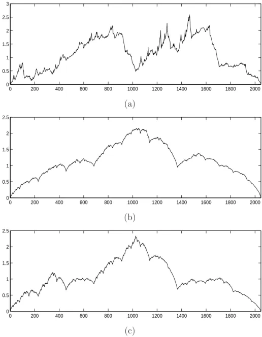
Brownian motion can be constructed as a CEBP, so MEBP include a class of time changed Brownian motion, suggesting their suitability for modelling purposes. We also propose to imitate an fBm with an MEBP. Proofs of the existence and continuity of MEBP are given, together with an efficient on-line algorithm for simulating them (a Matlab implementation is freely available from the web page of Jones). Also, using an approach of Riedi, an upper bound on the multifractal spectrum of the time change is derived (Chapter 4). Estimation of the spectrum using the wavelet leaders is also carried out, supporting the theoretical results. Further results about the Hausdorff spectrum of the time change defined on the boundary of the crossing tree are also obtained.
Galton-Watson Iterated Function
Systems
The terminology Iterated Function Systems (IFS), introduced by Barnsley and Demko [15], refers to a finite set of contractive mappings which completely spec-ify a fractal set. The study of IFS was pioneered by Hutchinson in 1981 [60] and Barnsley and coworkers. Hutchinson proved the existence of a unique fractal set and measure of an IFS using a contraction mapping principle, whereas Barnsley proved the same result using a probabilistic set up. In the first section of this chapter, we review the basic construction of fractal sets and measures using IFS. We mainly focus on the method proposed by Hutchinson since it will be relevant for the pro-posed extension in a later section. In addition, we briefly review alternatives to the construction of IFS, like Recursive Iterated Function Systems (RIFS), and explain how to add randomness to the model. In the second section we consider the space of p integrable functions and define a set of contractive mappings acting over this space, using the approach developed in [63]. These IFS rely on an M-ary underlying construction tree, if M is the total number of contractions used. We propose to ex-tend the model by allowing a random construction tree, with random contractions. The existence of a unique fixed point is shown following the approach of Hutchinson and Rüschendorff. Properties of the fixed point are described in section 2.5.
2.1
Self-similar sets and measures
In this section we review the definition and construction of self-similar sets. But first, we recall fundamental mathematical notions such as complete metric spaces, the fixed point theorem and the Hausdorff metric.
2.1.1
Contractive operators in metric spaces
Let X be a space and define a metric d : X × X → R on this space. (X, d) is then called a metric space. The concept of metric leads to the notion of convergence. A sequence of points (xn)n∈N of X is said to converge to an element of X when
the distance determined by the metric d between the two elements can be made arbitrarily small by sending n to infinity. We are mainly concerned with sequences
known as Cauchy sequences, which satisfy
∀ǫ > 0 ∃r ∈ N ∀(p, q) ∈ N2 p > r q > r ⇒ d(x
p, xq) 6 ǫ
where (xn)n∈N is a sequence of X. The definition of a Cauchy sequence states that
the distance between 2 elements of the sequence can be made arbitrarily small if we consider p and q large enough. Note that a Cauchy sequence does not necessar-ily converge. A metric space for which every Cauchy sequence converges is called complete.
Definition 2. If f : X→ X, we define the Lipschitz constant of f by
Lip(f ) = sup
x6=y
d(f (x), f (y)) d(x, y) .
f is Lipschitz if Lip(f ) <∞ and f is contractive if Lip(f) < 1
The following theorem plays a central role in the theory of Iterated Function Sys-tems. It is known as the Banach fixed point theorem.
Theorem 1. Let (X, d) be a complete metric space and f a contractive map. Then
f possess a fixed point in X. Moreover, this fixed point is unique.
2.1.2
Complete space of compact sets
Let K ⊂ R2. Suppose
• K is bounded, that is there exists r > 0 such that for all x∈ K, d(x, 0) 6 r. • K is closed. A set K is closed if its complement Kc is open, that is if for all
x ∈ Kc, there exists r > 0 such that B(x, r) ⊂ Kc, where B(a, r) is the open
ball of center a and radius r.
K is compact if and only if for every sequence (xn)n∈N, it is possible to extract
a subsequence which converges in K. It is a standard result that if the underlying space is of finite dimension, then K is compact if and only if K is closed and bounded. The set of compact subsets of R2 is usually denoted H(R2).
Let x ∈ R2 and S ∈ H(R2). Define the distance between x and K ∈ H(R2) by
d(x, K) = inf{d(x, y) | y ∈ K}
and the distance between K and S by d(K, S) = inf{d(x, S) | x ∈ K}. Then, define the Hausdorff metric on compact subsets of R2 by
dH(K, S) = sup{d(K, S), d(S, K)}.
It follows that (H(R2), d
H) is a complete metric space (see for example [14]). This
result motivates the study of sequences of compact sets defined via contraction mappings and the definition of IFS and self-similar sets.
2.1.3
Construction of self-similar sets
Consider a finite set {ω1, . . . , ωM} of contraction maps R2 → R2. If K ∈ H(R2),
define the scaling law W by
W (K) =
M
[
i=1
ωi(K).
Denote by si the Lipschitz constant of ωi. W is contractive with Lipschitz constant
s = max{s1, . . . , sM}. Using the terminology of Hutchinson and Rüschendorff, K∗
satisfies the scaling law W if K∗ = W (K∗) [63]. Such a set is by construction discrete
self-similar, since it can be decomposed into a union of scaled identical M copies of itself. They proved the existence of a unique self-similar set K∗ using the contraction
mapping theorem [60]. The Hausdorff dimension r of K∗ is usually fractional and
satisfies
M
X
i=1
sri = 1.
Let Wp(K) = W (Wp−1(K)). Starting from an arbitrary initial bounded set K 0 6= ∅,
Hutchinson proved that Wp(K
0) → K∗ in the Hausdorff metric. K∗ is therefore
known as the fixed point or the attractor of the IFS. This gives an algorithm to generate approximations of K∗. Select a starting point x
0 and define K0 = {x0}.
Let K1 = W (K0), K2 = W (K1), and so on. As n→ ∞, dH(Kn, K∗)→ 0. So for n
large enough, we can obtain a good approximation of the attractor.
Pictures of K∗ can also be obtained through a random and faster procedure, called
the ‘Random Iteration’ or ‘Chaos game’ [14, 15]. Consider an initial point x0and
ap-ply a contractive mapping ωi1 chosen uniformly among the M possible contractions.
x1 = ωi1(x0). Select again another transformation, independently from the previous
one, and apply it to x1. Repeat the procedure many times to obtain a sequence
of points. It is a famous result that the orbit {xn} is dense in K∗. This random
algorithm can be slightly modified by not picking ωk with uniform probability but
with probability pk, withPkpk= 1. The orbit still converges to the attractor of the
IFS, however some regions of the fixed point are visited more than others, depending on the values of pk. In fact the random algorithm generates a picture of a measure
µ, as suggested by the relation [42] µ(B) = lim n→∞ 1 n + 1 n X k=0 χB(xk)
where χB is the characteristic function of B. This equality makes explicit the
rela-tion between a measure, which support is the attractor of the IFS and the relative visitation frequency of a set B. This notion is made precise using the notion of self-similar measure, and it was proved in [60] that the measure µ previously obtained is the unique self-similar measure µ of total mass one, such that
µ =
M
X
i=1