A new horizon for the recommendation: Integration of spatial dimensions to aid decision making

(1)

HAL Id: tel-01422348

https://tel.archives-ouvertes.fr/tel-01422348

Submitted on 25 Dec 2016

HAL is a multi-disciplinary open access archive for the deposit and dissemination of sci-entific research documents, whether they are pub-lished or not. The documents may come from teaching and research institutions in France or abroad, or from public or private research centers.

L’archive ouverte pluridisciplinaire HAL, est destinée au dépôt et à la diffusion de documents scientifiques de niveau recherche, publiés ou non, émanant des établissements d’enseignement et de recherche français ou étrangers, des laboratoires publics ou privés.

spatial dimensions to aid decision making

Rajani Chulyadyo

To cite this version:

Rajani Chulyadyo. A new horizon for the recommendation: Integration of spatial dimensions to aid decision making. Computer science. Université de Nantes, 2016. English. �tel-01422348�

(2)

Thèse de Doctorat

Rajani C

HULYADYO

Mémoire présenté en vue de l’obtention du grade de Docteur de l’Université de Nantes

sous le label de l’Université de Nantes Angers Le Mans

École doctorale : Sciences et technologies de l’information, et mathématiques Discipline : Informatique et applications, section CNU 27

Unité de recherche : Laboratoire d’informatique de Nantes-Atlantique (LINA) Soutenue le 19 octobre 2016

A new horizon for the recommendation

Integration of spatial dimensions to aid decision making

JURY

Rapporteurs : M. Christophe GONZALES, Professeur des universités, Université Pierre-et-Marie-Curie (Paris VI)

M. Nicolas LACHICHE, Maître de conférences, Université de Strasbourg Examinateurs : M. ColinDE LAHIGUERA, Professeur, Université de Nantes

Mme_{Armelle B}_RUN_{, Maître de conférences, Université de Lorraine}

Invité : M. Cédric HOUSSIN, Directeur, DataForPeople

(3)

(4)

Acknowledgments

This thesis would not have been possible without the inspiration and continuous sup-port of a number of people.

I would like to express my deep gratitude to Prof. Philippe Leray for his supervision of my thesis. His continuous guidance, suggestions, and optimism over the last years have been invaluable to advance in my research. I feel very fortunate to be advised by him and to benefit from his expertise on this interesting area of research.

I am very grateful to DataForPeople for supporting this research. My special thanks go to Mr. Romain Perruchon, former CTO of DataForPeople, and Mr. Cédric Houssin, CEO of DataForPeople, for their guidance on the professional aspect of this thesis. Their expertise in the projects of DataForPeople has been a great help during the thesis. I am thankful to both of them as well as Mr. Pierre-Yves Huan, COO of DataForPeople, for creating a cordial working environment and helping me to inte-grate to the world of start-ups.

I would like to express my sincere gratitude to my colleagues, Anthony Coutant, Mouna Ben Ishak, and Thomas Vincent, for always sharing their expertise and experiences, and making the development of PILGRIM fun. Their domain expertise has helped me get good insights of PILGRIM.

Additionally, I am very thankful to my friends, Prajol and Trija for making me feel home away from home, Amandine and Mickaël for helping me learn French, and Amit, Niroj and Parbati for their company and emotional support.

I would also like to thank all those who have been helped me directly or indirectly in all stages of this thesis.

More than anything else, I am deeply grateful to my mom, dad, brother, and husband for their love and continuous moral support.

Thanks!

(5)

(6)

I

State-of-the-art

9

2 Probabilistic Relational Models for Relational Learning 11 2.1 Introduction . . . 12

2.2 Background . . . 13

2.2.1 Relational data representation . . . 13

2.2.2 Bayesian Networks . . . 16

2.3 Probabilistic Relational Models (PRMs) . . . 20

2.4 Extensions . . . 24

2.4.1 PRM with structural uncertainty . . . 24

2.4.2 Other extensions . . . 24

2.5 Inference in PRMs . . . 24

2.6 Learning PRMs . . . 25

2.6.1 Learning parameters . . . 25

2.6.2 Learning structure . . . 26

2.7 Evaluating PRM learning algorithms . . . 28

2.7.1 Evaluation strategy and metrics . . . 29

2.7.2 Generating PRM benchmarks . . . 30

2.7.3 Limitations . . . 31

2.7.4 Proposals for improvement . . . 32

2.8 Conclusion . . . 40

3 Recommender Systems: A Common Application of Relational Data 41 3.1 Introduction . . . 42

3.2 Recommendation models and techniques . . . 43

3.2.1 Recommendation data . . . 44

3.2.2 Recommendation techniques . . . 45

3.2.3 New developments . . . 51

3.3 Evaluation of recommender systems . . . 51

3.3.1 Evaluation approaches . . . 52

3.3.2 Accuracy metrics . . . 52

3.3.3 Other evaluation metrics . . . 54

3.3.4 Benchmark datasets and evaluation tools . . . 55 iii

(7)

3.4 Challenges . . . 57

4 Using Probabilistic Relational Models for Recommendation 61 4.1 Introduction . . . 62

4.2 Existing approaches . . . 62

4.2.1 Collaborative Filtering using PRMs (Getoor and Sahami [1999]) 62 4.2.2 A unified recommendation framework based on PRMs (Huang et al. [2004]) . . . 63

4.2.3 Hierarchical Probabilistic Relational Models (hPRM) (Newton and Greiner [2004]) . . . 64

4.2.4 Combining User Grade-based Collaborative Filtering and PRMs (UGCF-PRM) (Gao et al. [2007]) . . . 65

4.2.5 A RBN-based recommender system architecture (Ben Ishak et al. [2013]) . . . 65

4.3 Comparison and discussion . . . 66

5 Spatial Data 71 5.1 Introduction . . . 72

5.2 Spatial data representation . . . 72

5.2.1 Tessellation data representation . . . 73

5.2.2 Vector data representation . . . 73

5.2.3 Network data type . . . 74

5.3 Characteristics of spatial data . . . 75

5.3.1 Spatial heterogeneity . . . 75 5.3.2 Spatial autocorrelation . . . 75 5.4 Spatial operators . . . 76 5.4.1 Metric operators . . . 76 5.4.2 Topological operators . . . 76 5.5 Conclusion . . . 78

6 Recommender Systems with Spatial Data 79 6.1 Introduction . . . 80

6.2 Review of some spatial recommender systems . . . 80

6.3 Discussion . . . 82

II

Contributions

85

7 A Personalized Recommender System 87 7.1 Introduction . . . 88

7.2 The proposed approach . . . 90

7.2.1 PRM for preference-based recommendation (PRM-PrefReco) . . 90

7.2.2 Personalization . . . 93

7.2.3 Relational attributes and types of model . . . 96

7.2.4 Examples . . . 98

7.3 Experiments . . . 101

(8)

CONTENTS v

7.3.2 Experiment methodology . . . 102

7.3.3 Evaluation metrics . . . 102

7.3.4 Results and discussion . . . 103

8 PRM with Spatial Attributes (PRM-SA) 105 8.1 Introduction . . . 106

8.2 Definitions . . . 106

8.3 Learning PRM-SA . . . 112

8.4 Evaluation of PRM-SA learning algorithms . . . 116

8.4.1 Evaluation strategy and metrics . . . 117

8.4.2 Generation of PRM-SA benchmarks. . . 117

8.5 Experimental study . . . 122

8.5.1 Methodology . . . 123

8.5.2 Results and discussion . . . 126

8.6 PRMs-SA in recommender systems . . . 131

8.7 Conclusion . . . 132 9 Implementations in PILGRIM 135 9.1 An Introduction to PILGRIM . . . 136 9.2 Technical aspects . . . 137 9.3 PILGRIM-Relational . . . 137 9.3.1 Modules . . . 139 9.3.2 Implementation of PRM-SA . . . 144

9.3.3 Implementation of PRM benchmark generation . . . 145

9.4 PILGRIM-Applications . . . 148

10 Conclusion 151

III

Appendices

155

A Empirical Study of PRM Sampling Algorithms 157 A.1 Empirical study of relational block Gibbs sampling algorithm. . . 157

A.1.1 Methodology . . . 157

A.1.2 Results and discussion . . . 160

A.2 Comparison of sampling algorithms . . . 162

A.2.1 Methodology . . . 162

A.2.2 Results and discussion . . . 163

A.3 Conclusion . . . 165

B Using PILGRIM 167 B.1 Defining a PRM(-SA) . . . 167

B.1.1 Defining a relational schema . . . 167

B.1.2 Defining a dependency structure. . . 170

B.1.3 Defining parameters . . . 174

B.2 Instantiating a PRM for making inference . . . 175

B.3 Utility methods . . . 176

(9)

B.3.2 Exporting a relational schema into a database . . . 176

B.4 Generating datasets from a PRM . . . 176

B.4.1 Generating a random skeleton . . . 177

B.4.2 Sampling a PRM . . . 177

B.5 Working with PILGRIM-Recommender . . . 179

B.5.1 Defining a recommendation model. . . 179

B.5.2 Making recommendations . . . 181

(10)

List of Tables

2.1 Notations and their meaning . . . 14

3.1 Some datasets used for recommendation systems research purposes . . 56

4.1 Comparison of some PRM-based recommendation approaches . . . 68

5.1 Examples of spatial operators . . . 77

6.1 Comparison of some recommender systems that exploit spatial data . . 83

7.1 The scale of absolute numbers for expressing the relative importance of

a pair of decision factors (Saaty [2008]) . . . 95

7.2 CPD of P (Tx.DF_furnished | Search.furnished, Tx.Property.furnished) . 99

7.3 Evaluation result . . . 104

8.1 Average ± standard deviation of metrics for four PRM-SA structure

learning algorithms in the experiment. . . 128

8.2 Average ± standard deviation of metrics to measure spatial influence in

the learned models . . . 129

9.1 PILGRIM modules, and contributions made by the team members . . . 138

9.2 Summary of major functionalities implemented in PILGRIM-Relational 140

9.3 Summary of major functionalities implemented in PILGRIM-Recommender149

C.1 Average ± standard deviation of Hard Precision for PRM-SA structure

learning algorithms for models of Figure 8.6. . . 183

C.2 Average ± standard deviation of Hard Recall for PRM-SA structure

C.3 Average ± standard deviation of hard F-score for PRM-SA structure

C.4 Average ± standard deviation of Soft Precision for PRM-SA structure

C.5 Average ± standard deviation of Soft Recall for PRM-SA structure

learn-ing algorithms for models of Figure 8.6. . . 185

C.6 Average ± standard deviation of Soft F-score for PRM-SA structure

C.7 Average ± standard deviation of Soft Precisionskeleton of models of

Fig-ure 8.6. . . 186

C.8 Average ± standard deviation of Soft Recallskeleton of models of Figure 8.6186

C.9 Average ± standard deviation of Soft F-scoreskeletonof models of Figure 8.6186

C.10 Average ± standard deviation of Hard Precisionspatial of models of

Fig-ure 8.6 . . . 187

(11)

C.11 Average ± standard deviation of Hard Recallspatial of models of Figure 8.6187

C.12 Average ± standard deviation of hard F-scorespatial of models of Figure 8.6187

C.13 Average ± standard deviation of Soft Precisionspatial of models of Figure 8.6188

C.14 Average ± standard deviation of Soft Recallspatial of models of Figure 8.6188

C.15 Average ± standard deviation of Soft F-scorespatial of models of Figure 8.6189

C.16 Average ± standard deviation of normalized mutual information(NMI) between the spatial partition learned during the experiment, and the original spatial partition for the spatial attribute (User.location) of each

model of Figure 8.6 . . . 189

C.17 Absolute difference between Bayesian Dirichlet score of the gold models

(12)

List of Figures

2.1 (a) An example of a relational schema, (b) Crow’s foot notations . . . . 15

2.2 Instantiations of the relational schema of Figure 2.1a . . . 17

2.3 An example of a Bayesian network (Pearl [1988]) . . . 18

2.4 An example of a PRM corresponding to the relational schema of

Fig-ure 2.1a . . . 22

2.5 Ground Bayesian network obtained by unrolling the PRM of Figure 2.4

over the relational skeleton of Figure 2.2 . . . 23

2.6 Class dependency graph of the PRM in Figure 2.4 . . . 23

2.7 Overview of PRM benchmark generation process proposed by Ben Ishak

[2015]. . . 31

2.8 (a) Relational schema DAG of Figure 2.1a (considering only three classes),

(b) Relational skeleton of Figure 2.2a as a k-partite graph . . . 33

2.9 A dummy relational schema: (a) Entity-Relationship diagram, (b) as a

directed graph . . . 37

2.10 Generating objects while performing Depth First Search (DFS) on the relational schema. This shows one iteration of a DFS performed on the

schema. . . 38

2.11 Next two iterations of DFS on the relational schema of Figure 2.9 fol-lowing the first iteration of Figure 2.10 to generate relational skeleton

graph. . . 38

3.1 Data representations commonly used in recommender systems . . . 45

3.2 Recommendation approaches. . . 47

3.3 Hybridization techniques (Burke [2007], Jannach and Friedrich [2013]) . 49

4.1 A Bayesian network for two-sided clustering (Getoor and Sahami [1999]) 63

4.2 (a) Hierarchy of Movie class and (b) Hierarchical Probabilistic Relational

Model (hPRM) proposed by Newton and Greiner . . . 64

4.3 Overview of the recommender approach proposed by Gao et al. [2007] . 65

4.4 The overall architecture of the recommender system proposed by Ben Ishak

et al. [2013] . . . 66

4.5 Sample hierarchies an hPRM cannot address . . . 67

5.1 Examples of spatial data . . . 74

6.1 Partial pyramid structure proposed by Levandoski et al. [2012] for

par-titioning users based on their location. . . 81

6.2 An example of a location-based social network graph (Wang et al. [2013]) 82

7.1 Relational schema of our proposed preference-based recommender system 91

(13)

7.2 The proposed PRM (a) before introducing decision factors, and (b) after

introducing decision factors. . . 93

7.3 Three types of proposed recommendation model . . . 97

7.4 (a) A screenshot of Kyzia, (b) Relational schema of Kyzia, (c) PRM-PrefReco for Kyzia. . . 99

7.5 Re-formulation of Delcroix and Ben Mrad [2016]’s approach of modeling decision criteria by V-structures in a Bayesian network into a PRM-PrefReco . . . 101

8.1 (a) An example of a relational schema with a spatial attribute Restaurant. (b) The relational schema adapted for the spatial attribute Restaurant.location. (c) A PRM-SA as proposed in Definition 23 . . . 108

8.2 The class dependency graph for the PRM-SA in Figure 8.1c . . . 111

8.3 An example of a class dependency graph with a cycle . . . 111

8.4 An example of a dependency structure that models the dependency of an attribute with the aggregated value of the same attribute of spatial objects in the same cluster. . . 112

8.5 (a) A PRM-SA with multiple spatial attributes. (b) The corresponding moralized graph used to identify the set of partition functions to be optimized. . . 115

8.6 PRMs-SA used in the experiments as gold standard models. . . 124

8.7 Comparison of overall performance of PRM-SA learning algorithms with Nemenyi test . . . 129

8.8 Comparison of overall hard precisionspatial, soft precisionspatial and soft recallspatial of PRM-SA learning algorithms with Nemenyi test . . . 130

8.9 Result of Nemenyi test for comparison of overall performance of PRM-SA learning algorithms in terms of the difference between the score of learned models and that of gold models. . . 130

9.1 Technological stack diagram . . . 139

9.2 Class diagram showing how RelationalSchema, Class, Attribute, and Domain are related to each other . . . 141

9.3 Class diagram showing how RBN is related to other classes . . . 142

9.4 Types of RBNDistribution . . . 143

9.5 Class diagram of RGS . . . 146

9.6 Types of GraphOperation available in PILGRIM-Relational . . . 146

9.7 Class diagram of relational skeleton generation strategies implemented in PILGRIM. . . 147

9.8 Class diagram of sampling strategies implemented in PILGRIM . . . . 148

9.9 Class diagram of RecoModel . . . 149

9.10 Class diagram of NaiveBayesianClassifier . . . 150

A.1 (a) The PRM used in the experiments, and (b) the underlying relational schema as a DAG . . . 158

A.2 Distribution of objects in the relational skeletons used in the experiments159 A.3 Max in-degree of entity objects in the relational skeletons. . . 160

A.4 Distribution of in-degree in naïve and k-partite skeletons . . . 160

A.5 Burn-in vs time taken by RBG sampling algorithm on naïve and k-partite graph-based skeletons of different size. . . 161

(14)

LIST OF FIGURES xi A.6 Skeleton size vs time taken by RBG sampling algorithm for different

values of burn-in. . . 162

A.7 Skeleton size vs number of nodes that rejected the null hypothesis of the Chi-square goodness-of-fit test for different values of burn-in. Lower

values are better here. . . 163

A.8 Burn-in vs number of nodes that rejected the null hypothesis of the Chi-square goodness-of-fit test on (a) k-partite graph-based skeletons, and

(b) naïve skeletons of different size. Lower values are better here. . . . 164

A.9 Time taken by relational forward sampling, RBG sampling, and GBN-based sampling algorithms on naïve and k-partite graph-GBN-based skeletons

of different size. . . 164

A.10 Number of nodes that rejected the null hypothesis of the Chi-square goodness-of-fit test on naïve and k-partite graph-based skeletons of

dif-ferent size. Lower values are better here. . . 165

C.1 Comparison of PRM-SA learning algorithms with Nemenyi test for Model

A1 . . . 191

A2 . . . 191

C2 . . . 192

(15)

(16)

List of Algorithms

1 Generate_Neighbors (Bayesian Networks) . . . 20

2 Lazy Aggregation Block Gibbs (LABG) . . . 25

3 Relational Greedy Search. . . 26

4 Generate_Neighbors (PRM) . . . 27

5 Generate_Random_PRM-DB (Ben Ishak [2015]) . . . 32

6 Generate_Relational_Skeleton . . . 34

7 Generate_SubSkeleton . . . 36

8 Relational forward sampling . . . 39

9 Relational Block Gibbs sampling (based on Kaelin [2011]’s LABG). . . 40

10 Generate_Neighbors (Naïve Approach) . . . 113

11 Increase_k Operation. . . 113

12 Decrease_k Operation . . . 114

13 Find_Structure_With_Best_k . . . 116

14 Adaptative_Structure_Learning (Version 1) . . . 116

15 Adaptative_Structure_Learning (Version 2) . . . 117

16 Generate_Neighbors (Adaptative Structure Learning Version 3) . . . . 118

17 Generate_PRM-SA_Benchmark . . . 119

18 Generate_Spatial_Schema . . . 120

19 Generate_Spatial_Relational_Dataset . . . 121

20 Generate_Spatial_Relational_Skeleton. . . 121

(17)

(18)

Abbreviations

AHP Analytical Hierarchical Process. 81, 83,95

AIC Akaike Information Criterion. 19, 136

BD Bayesian Dirichlet. 19

BIC Bayesian Information Criterion. 19,136

BN Bayesian Network. 3,12,13,16,18–20,24,26,28,38,66–68,80,81,83,100,101,

106, 121, 154

CARS Context-aware Recommender System. 44, 45

CDG Class Dependency Graph. 22

CF Collaborative Filtering. 45, 46, 57, 65,67–69, 80,83

CI Conditional Independence. 19, 20

CPD Conditional Probability Distribution. 16, 18, 21, 24, 25, 30–32, 39, 92–94, 98,

139, 141, 145, 147, 167, 174

CRP Chinese Restaurant Process. 33,35

DAG Directed Acyclic Graph. 3, 19,29–31, 33–36,118, 124, 125, 147, 157–160, 169

DAPER Directed Acyclic Probabilistic Entity Relationship. 30, 117, 124, 133, 154

DF Decision Factor. 92

DFS Depth-First Search. 34–36

DMMHC Dynamic Max-Min Hill Climbing. 136

DMMPC Dynamic Max-Min Parents and Children. 136

DSS Decision Support System. 42

DTL Database Template Library. 137

DUKe Data, User and KnowledgE. 136

EAP Expectation a Posteriori. 19, 143

ERD Entity-Relationship Diagram. 15

GBN Ground Bayesian Network. 21, 24, 25, 30–32, 35, 37, 39, 40, 94, 109, 110, 118,

121, 122, 128, 137, 139, 140, 143, 148, 153,154,157,162–165, 175

GIS Geographic Information System. 80

GPS Global Positioning System. 72

HCI Human-Computer Interaction. 50

hPRM Hierarchical Probabilistic Relational Model. 24, 64, 67,69

(19)

IDG Instance Dependency Graph. 22, 32

IR Information Retrieval. 42, 52, 54

KNN K-Nearest Neighbors. 81, 83

LABG Lazy Aggregation Block Gibbs. 25, 32,39, 40, 118, 122, 153, 154

LINA Laboratoire d’Informatique de Nantes Atlantique. 136

LSI Latent Semantic Indexing. 57

MAE Mean Absolute Error. 53, 67–69

MAP Maximum a Posteriori. 16, 19, 143

MAUT Multi-Attribute Utility Theory. 50

MBR Minimum Bounding Rectangle. 76

MCDM Multi-criteria Decision Making. 50,94

MDL Minimum Description Length. 19, 136

ML Machine Learning. 42

MLE Maximum Likelihood Estimation. 19, 25, 143

MMHC Max-Min Hill Climbing. 20,26, 136

MML Minimum Message Length. 19

MMPC Max-Min Parents and Children. 20, 136

NMAE Normalized Mean Absolute Error. 53

NMI Normalized Mutual Information. 126, 130, 183

OGC Open Geospatial Consortium. 76

OOBN Object-Oriented Bayesian Network. 3, 80

PCA Principle Component Analysis. 57

PGM Probabilistic Graphical Model. 2,3

POI Point-of-interest. 56,81

PPR Personalized PageRank. 82

PRM Probabilistic Relational Model. 3–8, 12, 13, 20, 24, 28, 62–69, 89, 90, 92–94,

104, 106,111,112, 117,125,132, 133, 136,137,139, 141,143–145,148, 151–154, 157, 158, 167, 170, 171,174–178

PRM-CH Probabilistic Relational Model with Class Hierarchy. 24, 64,67

PRM-CU Probabilistic Relational Model with Clustering Uncertainty. 24, 136, 138,

141, 144, 172

PRM-EU Probabilistic Relational Model with Existence Uncertainty. 3, 24, 63, 69,

89–91

PRM-PrefReco Probabilistic Relational Model for Preference-based Recommenders.

90, 92–94, 96, 98–102, 151

PRM-RU Probabilistic Relational Model with Reference Uncertainty. 24, 26, 136,

(20)

Abbreviations xvii

PRM-SA Probabilistic Relational Model with Spatial Attributes. 5–8, 106,123, 124,

127–130, 132, 133, 136–138, 143–145, 148, 152–154, 167, 170, 172, 174, 175, 177, 178, 183, 191–193

RBG Relational Block Gibbs. 38, 39,122,123,138,148, 153, 157, 158, 161–165

RBN Relational Bayesian Network. 3, 29, 117

RDN Relational Dependency Network. 3

RGS Relational Greedy Search. 26, 124, 132, 133, 143, 145, 153

RMMHC Relational Max-Min Hill Climbing. 26,31, 133, 138, 143, 153

RMMPC Relational Max-Min Parents and Children. 133, 153

RMN Relational Markov Network. 3, 112

RMSE Root Mean Squared Error. 53

RS Recommender System. 3, 42–45, 48,51, 52, 54,58, 59, 62, 88–91, 106

RSHD Relational Structural Hamming Distance. 30, 117, 124

SRL Statistical Relational Learning. 2–4,12, 13, 153

ST-DBN State-and-transition Dynamic Bayesian Network. 80

SVD Singular Value Decomposition. 57

UGCF-PRM User Grade-based Collaborative Filtering - PRM. 65,67

VGI Volunteered Graphical Information. 72

WSM Weighted Sum Method. 94, 102, 103

(21)

(22)

Special Terms

k-partite graph A graph whose vertices can be partitioned into k disjoint sets so that

there is no edge between any two vertices within the same set. 33,118,123, 153,

157, 177

Markov blanket The Markov blanket of a node in a Bayesian network is the set of

parents, children, and spouses of the node. 63,69, 125

Moral Graph A moral graph is the equivalent undirected graph of a directed acyclic

graph and is obtained by adding an edge between the nodes that have a common

child and changing directed edges to undirected ones. 114

Skeleton of a DAG The skeleton of a directed acyclic graph is the undirected graph

that results from ignoring the directionality of every edge. 125

V-structure A v-structure in a directed acyclic graph G is an ordered triplet of nodes,

(x, y, z), such that G contains the arcs x → y and y ← z, and the nodes x and z

are not adjacent in G. 125

(23)

(24)

1 Introduction

1.1 Context

The increase in Internet users has become a global phenomenon. Almost all coun-tries in the world have witnessed the incredible growth of Internet users in the past

two decades1. These users not only consume the data available in the Internet but also

produce a huge amount of data through various activities, such as browsing, searching, providing personal information, blogging, sharing digital items (e.g., photos, videos etc.), volunteering (e.g., Wikipedia, OpenStreetMap), participating in surveys etc. Along with Internet users, the number of websites on the world wide web is also

grow-ing drastically2_{. Simultaneously, technologies for collecting, disseminating, processing,}

and analyzing data have been improving at a fast pace. The combined effect of all these is that a tremendous volume of data is available day by day. The source of data is not limited to the Internet only. Various domains, such as environmental, biologi-cal, economical studies, and many applications contribute to the ever increasing data. With this abundance of data, extracting knowledge or useful information from data has become a widely researched topic.

Data analysis and knowledge discovery involve methods at the intersection of ma-chine learning, statistics and databases. Mama-chine learning is concerned with the ex-traction of knowledge in the form of functions, mathematical or statistical models that automatically evolve with experience. It is largely dominated by inductive learning (also known as learning from examples or learning by induction) techniques, which aim at inducing patterns (or hypotheses) from the given input data for predicting new data (predictive modeling) or for describing the input data (descriptive modeling). Traditional machine learning techniques are designed to work with attribute-value

rep-resentation of data (also known as single-table single-tuple (Raedt [2008]) format or

propositional data), where each row represents a data instance, and each column repre-sents an attribute. These techniques also assume that the data instances are indepen-dent and iindepen-dentically distributed (IID), i.e., the data instances are drawn indepenindepen-dently from each other from an identical distribution. Examples of such dataset include

well-known Iris dataset3_{, mushrooms dataset}4 _{etc., which have been used in many studies.}

However, in general, real-world data do not come in single-table format. It has been a common practice to conceptualize a real-world system in terms of objects and relation-ships between those objects. That means real-world data usually come as multi-table

multiple-tuple (Raedt [2008]) data, also called relational data. This kind of data

con-sists of multiple tables, each corresponding to an entity type or a relationship type. Each row in an entity table represents an entity/object, and each row in a relationship table denotes the relationship between objects. As objects are related to each other, the IID assumption is often violated in relational data. This limits the application of

traditional machine learning algorithms on relational data. Consequently, Statistical

Relational Learning (SRL) has been emerged as a branch of machine learning that is

concerned with statistical analysis on domains with complex relations and uncertainty

(Getoor and Taskar [2007]).

SRLaims at learning statistical models exploiting relational information present in

the data. It is primarily dominated by methods that are based on Probabilistic

Graph-ical Models (PGMs). PGMs use graph theory for expressing complex probabilistic

1. http://data.worldbank.org/indicator/IT.NET.USER.P2

2. http://www.internetlivestats.com/total-number-of-websites/

3. https://archive.ics.uci.edu/ml/datasets/Iris

(26)

1.1. CONTEXT 3

dependencies between random variables (Wainwright and Jordan [2008]). Directed as

well as undirected versions of PGMs have been extended for relational settings.

Prob-abilistic Relational Models (PRMs) (Friedman et al. [1999], Getoor [2001]),Relational

Bayesian Networks (RBNs) (Jaeger [1997]), and Object-Oriented Bayesian Network

(OOBN)(Koller and Pfeffer[1997],Bangsø and Wuillemin[2000]) are relational

exten-sions of Bayesian Networks (BNs), which are PGMs that use Directed Acyclic Graphs

(DAGs). Markov networks, and dependency networks, which are respectively

undi-rected and bi-diundi-rected counterparts ofBNs, have been extended by Relational Markov

Networks (RMNs)(Taskar et al.[2002]), andRelational Dependency Networks (RDNs)

(Neville and Jensen [2007]) respectively with the concept of objects to deal with

re-lational data. This thesis is concerned with the directed version, particularly PRMs.

A PRM models the uncertainty over the attributes of objects in the domain and the

uncertainty over the relations between objects (Friedman et al. [1999]).

SRL has found its application in special tasks that originate from the relational

nature of data. Most popular among these tasks are link prediction, entity resolution, collective classification, and link-based clustering. The central idea to all of them is to exploit links (or relationships) between objects for problem solving. Links can be, for example, the action of rating/buying an item in an e-commerce website, friendships in social networks, the action of reading news articles/listening to music, co-author links between author references in bibliographical data, links between spatial references in geo-spatial data and so on. The objective of link prediction is to determine whether a link or relationship exists between objects. Entity resolution aims at identifying references that denote the same entity. Practical uses of entity resolution include finding duplicates in data, integrating data from multiple sources, disambiguating user queries etc. The goal of collective classification is to classify entities given their attributes and links in presence of autocorrelation. Link-based clustering groups together objects based on the similarity of their attributes as well as the attributes of linked objects.

In this thesis, we are particularly interested in the task of link prediction. One of the

applications where link prediction is very useful isRecommender Systems (RSs), which

is also a very common source of relational data. Recommender systems are basically built around the interaction between users and items, and help discover interesting items for users from a big collection of items. Such systems can be observed in many different websites that we use everyday (e.g., Amazon, YouTube, IMDb, Facebook etc.). In general, users are described by some properties such as their demographics information. Items are domain-specific objects that users are looking for, such as music, movies, books, news, cities, restaurants, friends, products etc. Depending on the domain, users might interact with items in different ways. For example, in Amazon, users purchase items, and provide feedback in the form of ratings, and comments; in social networking sites, users become friends. The goal of a recommender system is to predict the items that users might find interesting to interact with. In other words, recommender systems predict whether a link could exist between a user and an item.

Probabilistic Relational Model with Existence Uncertainty (PRM-EU), an extension of

PRMfor modeling the uncertainty over the existence of relationships between objects,

can be suitable in such scenario.

As recommender systems have the potential to increase revenue generation, they are being applied in many different systems. Consequently, various recommendation tech-niques have been devised to fit in different scenarios. A growing trend in recommender systems is to improve recommendations by exploiting locational or spatial information about users and/or items. For example, YouTube recommends videos that are popular

(27)

in users’ geographic region, LinkedIn suggests jobs in nearby areas etc. The presence of a spatial dimension enhances users’ experience. At the same time, it restrains the application of conventional algorithms because of the geographical representation of objects and the interactions it adds between objects. Such interactions make

multi-relational settings suitable for analyzing spatial data (Malerba[2008]). ThoughPRMs

are interesting SRL models that can extract statistical patterns from relational data,

they cannot treat spatial objects in the same way as non-spatial ones due to the pres-ence of spatial information, which are commonly represented through their geometry.

Malerba [2008] has mentioned the possibility of using PRMs with spatial relational

databases. However, not much progress has been made in this direction.

This thesis deals with the (not much explored) intersection of three related fields –

PRMs, spatial data, and recommender systems. The thesis makes two main

contribu-tions. Our first contribution is concerned with the intersection of PRMs and

recom-mender systems. We propose a novel approach for usingPRMsfor making personalized

recommendations in preference-based systems. Our second contribution addresses the

problem of integrating spatial information into PRMs. In the following section, we

will describe the motivating scenario for this thesis and state the problems we try to address.

1.2 Motivation and problem statement

As we have discussed in the previous section, PRMs can be used to realize

rec-ommender systems through the task of link prediction. Using PRMs in recommender

systems has, in fact, been a topic of research from the beginning of PRM formalism.

However, most of the studies (e.g., Getoor and Sahami [1999], Newton and Greiner

[2004]) are focused on implementing collaborative filtering approach, which demands a

good amount of historical data about users’ interactions in the system. In the absence

of such historical data, PRMsare used with users’ demographics information or items’

basic features (Gao et al. [2007], Huang et al. [2004]). At DataForPeople, a young

startup based in Nantes, there was a need for a recommender system for recommend-ing real estate properties, which are far less frequently purchased than books, movies

or similar inexpensive items. In this system, called Kyzia5_{, users provide their}

prefer-ences (or criteria for search) about various features of real estate properties. The goal is to recommend most relevant properties to the users from their search criteria. The system does not oblige users to provide their personal details because they usually have short-term preferences. So, users have very less interactions with this young system. Because of the lack of user profiles, and infrequent interactions of users, commonly used techniques, such as collaborative filtering or demographics-based filtering, are not appropriate for this system. Besides being short-term, an interesting but challenging property of users’ preferences in our system is that users may have different flexibility towards those preferences. In other words, users generally have preferences not only about items’ features but also about search criteria. For example, a user who does not have good income may be strict about his preferred price of properties but flexible about other features of properties whereas a user with children may not be willing to compromise the surface area of properties and so on. Such situations can arise not only in real estate search systems but also in other systems, such as flight/product search systems, hotel reservation system etc., where items are described by a set of features

(28)

1.2. MOTIVATION AND PROBLEM STATEMENT 5 and users state their preferences about those features to find their preferred items.

For similar domains, Viappiani et al. [2007], and Shearin and Lieberman [2001] have

proposed critiquing-based systems, where users are first presented with a small set of recommended items and the recommendations are iteratively improved after receiving feedback (or critiques) from the users. They take into account users’ preferences about feature values but not about search criteria. Moreover, such iterative solutions demand users’ patience to receive good recommendations. Therefore, the first contribution of this thesis deals with the problem of providing personalized recommendations, even without user profiles, to users from their preferences about items’ features and search criteria for recommending less frequently purchased (or interacted) items. We propose

a PRM-based solution for this problem. Our solution is generic and is not restricted

to the domain of real estates.

In the context of real estate recommendation, adding a spatial dimension is always interesting because real estate properties always involve geographical information, and users tend to have preferences about location. For example, users may prefer to live not too far from some points of interest such as workplace, children’s schools etc., and they may have different preferences for the geographical position and various other features of the property. Thus, adding a spatial dimension in a recommender system might improve the quality of recommendations. We identify two approaches to make use of spatial information in our recommendation system – (1) by integrating spatial information directly into our personalized recommendation model, and (2) by

enhanc-ing PRMs to support spatial objects and then use the enhanced PRMs instead of

standard PRMs in our recommendation model. The second approach is more general,

and can enablePRMs to be applied on spatial data not necessarily from recommender

systems only. Therefore, the second contribution of this thesis addresses the problem

of supporting spatial objects inPRMs. Our decision for taking the second approach is

also driven by the change in business model of DataForPeople. Our concentration was shifted from real-estate data to collaborative data collected from city-dwellers through

our mobile application FixMaVille6 _{to help improve their cities. Therefore, we now}

have a different kind of spatial data. To analyze general spatial data, we propose to

extend standard PRMs to support spatial objects. We formalize the new extension

of PRMs as Probabilistic Relational Models with Spatial Attributes (PRMs-SA), and

propose more than one algorithm for learning the structure of such models from spatial

data. To evaluate our proposed algorithms, we followBen Ishak[2015]’s methodology,

which involves the comparison of the model learned from a synthetic data with the

model from which the synthetic data is generated. Ben Ishak [2015] has proposed an

algorithm for generating random datasets for benchmarkingPRMlearning algorithms.

However, it only generates non-spatial datasets. Thus, we propose an algorithm for

generating spatial datasets by samplingPRMs-SA.

To summarize, following are the main research challenges that this thesis attempts to answer:

1. How to make personalized recommendations from users’ short-term preferences about items when :

— Items are less frequently purchased, i.e. low user-item interactions,

— Users have preferences not only for items but also for items’ various charac-teristics,

(29)

— The system lacks user profiles, i.e. no possibility of making recommendations based on demographics information, and

— The system is new with very few users?

2. How to integrate spatial information into aPRM? How to learn such probabilistic

models from spatial data?

3. How to generate spatial datasets randomly?

1.3 Contributions

This thesis has made the following contributions: A PRM-based, personalized recommender system

We have proposed a novel approach to build a personalizedPRM-based

recommen-dation model taking into consideration users’ preferences for items as well as for items’

characteristics (Chulyadyo and Leray [2014]). Using our generic approach,

content-based, collaborative filtering as well as hybrid models can be achieved from the same

PRM. Our preliminary experiment on a real-world dataset has shown that our model is

actually capable of personalizing recommendations in cold-start situation. This work

was presented at KES ’2014, and will be explained in detail in Chapter7.

PRM with spatial attributes (PRM-SA)

The second contribution of this thesis is the formalism of PRMs-SA, an extension

of PRMsto add a support for spatial data. We have also proposed some algorithms to

learn our model from data. The theoretical aspects of our model has been presented at

DSAA ’2016 (Chulyadyo and Leray [2015]). This thesis adds experiments to evaluate

our proposed algorithms for learning the structure of aPRM-SA. Chapter8will provide

an in-depth elaboration of our model, and present experimental findings. Improvement of PRM benchmark generation process

As algorithms for learning PRM-SAstructure can be evaluated in the same way as

those for PRMs, we tried to followBen Ishak[2015]’s approach. However, we

encoun-tered some limitations in their approach, which prevented us from utilizing their

al-gorithms for simulating spatial datasets to evaluate our PRM-SAlearning algorithms.

We have discussed these limitations in Section 2.7.3, and proposed some

improve-ments, notably algorithms for generating relational skeletons and sampling PRMs, in

Section 2.7.4. Our proposed algorithm for relational skeleton generation has been

il-lustrated in the technical report Ben Ishak et al. [2016]. We extended the improved

benchmark generation process to generate random spatial datasets, which are needed

for evaluating our PRM-SA learning algorithms. This will be explained in Section

8.4.2.

Development of PILGRIM software

One of the main objectives of this thesis is also to contribute in the development of a software tool to work with probabilistic graphical models. Our research lab, LINA, has been actively developing a tool called PILGRIM (ProbabIListic GRaphIcal

(30)

1.4. ORGANIZATION OF THE DISSERTATION 7

Model). Originally developed for modeling, learning and reasoning upon Bayesian

networks, this project was extended to supportPRMs. This thesis has made significant

contributions in the implementation and improvement of core functionalities as well

as the development of some modules of PILGRIM. Our proposed model, PRM-SA,

and algorithms for learning such model have also been implemented in PILGRIM.

To demonstrate the usage of PRM in practical applications, Huang et al. [2004]’s

recommendation model has been implemented. Chapter 9 will explain PILGRIM in

detail. Appendix B is provided as a user guide to illustrate the usage of PILGRIM

along with code snippets. Other contributions

Our state-of-the-art about PRM-based recommender systems has been presented

at Ben Ishak et al. [2014], and published in a technical report Chulyadyo and Leray

[2013].

An empirical study about PRM sampling algorithms was also performed during

this thesis. Details on this study and its findings are presented in Appendix A.

This thesis has also contributed to professional projects of DataForPeople, notably Kyzia and FixMaVille.

1.4 Organization of the dissertation

Chapter 2 will provide an introduction to relational data, and Bayesian networks.

We will define basic concepts used in the representation of relational data with some examples. We will present a general overview of Bayesian networks, and standard ap-proaches for learning such models. Then, we will define Probabilistic Relational Models

(PRMs), and related concepts. We will also present methods for learning aPRMfrom

data. We will then concentrate on evaluation ofPRMlearning algorithms, particularly

on the state-of-the-art methodology proposed by Ben Ishak[2015]. We will discuss on

some limitations of their approach, and propose some improvements.

Chapter 3will introduce recommenders systems, and will provide a review of

stan-dard recommendation techniques. We will then focus our discussion on the evaluation of recommender systems. We will also discuss on some major challenges imposed on recommender systems.

In Chapter 4, we will review some recommender systems that use PRMs. Through

this review, we show thatPRMs have the potential to be used for recommendations.

Chapter 5 will give a brief introduction to spatial data. We will explain basic

con-cepts related to spatial data, such as commonly used ways for representing spatial data, special characteristics of spatial data, and various operations that can be performed on this kind of data.

We will review some spatial recommender systems in Chapter 6 to show the trend

of using spatial information in recommender systems.

Chapter 7 will present our first major contribution of this thesis. We will present

(31)

our model in detail, and illustrate, through examples, that our approach is applicable in different domains. We will then present the findings of a preliminary experiment that we performed on our target application, which is a very new system with very few users.

Our second contribution, PRMs with Spatial Attributes (PRMs-SA), will be

pre-sented in Chapter 8. We will start with the definitions of PRMs-SA, and related

concepts. We will also propose four algorithms for learning the structure of a

PRM-SA. We will discuss on the methodology for evaluating those algorithms. We will then

present the results of the experiments performed to evaluate the four algorithms for

learning a PRM-SA.

Chapter 9 will provide a detailed insight into PILGRIM. It consists of four

sub-projects. But since this thesis has contributed in the sub-projects PILGRIM-Relational, and PILGRIM-Applications, we will discuss on the implementation of various modules of these two projects only.

In Chapter 10, we will present our conclusions, and point towards some prospects

of future research in the area addressed by this thesis.

Appendix A will present the experiments we had performed to study three PRM

sampling algorithms. The findings of this study were crucial for setting up the

experi-ments of Section 8.5 for evaluating PRM-SA learning algorithms.

Appendix B has been provided as a user guide to serve as a quick guide for those

who use our PILGRIM-Relational and PILGRIM-Applications libraries.

AppendixCwill provide the detailed results of our experiment for evaluating

(32)

I

State-of-the-art

(33)

(34)

2 Probabilistic Relational Models for

Relational Learning

2.1 Introduction

Nowadays it is very common to represent a system in terms of relationships between objects that exist in the system. It is, in fact, an intuitive approach to conceptualize systems because we often experience such relationships in our daily life. For example, a person is related to another person in a family, a cat is related to a person because he owns the cat, a webpage is often linked to other webpages, a movie may be related to a book because it is based on that book, and so on. Such relationships between different types of objects, referred to as relational data, have been the subject of analysis

in various domains, such as bioinformatics (Salwinski et al. [2004]), recommender

systems (Ricci et al.[2011],Bobadilla et al.[2013],Huang et al.[2005]), communication

analysis (Rossi and Neville [2010]), network analysis (Tang and Liu [2009], Chau and

Chen [2008]), scientific citation (Martin et al. [2013], Shibata et al. [2012], Popescul

and Ungar [2003]), natural language processing (Califf and Mooney [1999]) etc.

With the increased use and availability of relational data, the interest in extracting useful patterns from such data has been steadily growing in the machine learning com-munity. In traditional machine learning settings, data is usually assumed to consist of a single type of object, and the objects in the data are assumed to be indepen-dent and iindepen-dentically distributed (IID). The IID assumption, however, is often violated in a relational setting because of the presence of relationships between objects. This limits the application of traditional machine learning algorithms on relational data.

Consequently, Statistical Relational Learning (SRL) has been emerged as a branch of

machine learning that is concerned with statistical analysis on domains with complex

relations and uncertainty (Getoor and Taskar [2007]). SRLaims at learning statistical

models exploiting relational information present in the data. Application ofSRL

meth-ods can be found in the tasks of link prediction (Popescul and Ungar [2003], Huang

et al. [2005]), entity resolution (Nickel et al. [2011],Bhattacharya and Getoor [2007]),

collective classification (Neville and Jensen [2003],Macskassy and Provost[2007]), and

link-based clustering in relational context.

In the past two decades, significant advances have been made in the area of SRL.

A variety of SRLmodels has been proposed. Most of these models are based on

prob-abilistic graphical models (PGMs), a formalism for multivariate statistical modeling that uses graph theory for expressing complex probabilistic dependencies among

ran-dom variables (Wainwright and Jordan[2008]). Probabilistic relational models (PRMs)

(Friedman et al.[1999],Getoor et al.[2001]), and relational Bayesian networks (RBNs)

(Jaeger[1997]) are some of the earliest approaches toSRL1_{, and extend Bayesian}

net-works (BNs), a commonly used directed graphical model. Taskar et al.[2007] proposed

relational Markov networks (RMNs) based on Markov networks, an undirected

coun-terpart ofBNs. Other importantSRLmodels based on graphical models are relational

dependency networks (Neville and Jensen[2003]), which are based on dependency

net-works, Directed Acyclic Probabilistic Entity-Relation (DAPER) models (Heckerman

et al. [2004]), Markov logic networks (Richardson and Domingos [2006]), Bayesian

Logic Programs (Kersting and De Raedt [2007]) etc.

In this thesis, we focus on PRMs only. Since this model is an extension of BNsfor

relational data, we will begin with a brief overview of relational data representation

and BNs in the following section. We will then introducePRMs in Section 2.3.

1. PRMs are also referred to as RBNs in recent articles (Neville and Jensen [2003]). However, in this thesis, we preserve the original context and use PRM to refer to the model proposed byFriedman et al.[1999] andGetoor et al.[2001].

(36)

2.2. BACKGROUND 13

2.2 Background

As mentioned in Section 2.1, several models exist forSRL. These models are often

characterized by the representation of relational data and the tasks they address. As

we are concerned with PRMs only, we will present a review of the relational data

representation used by PRMs in Section 2.2.1, and the formalism of BNs, the basis of

PRMs, in Section2.2.2.

2.2.1 Relational data representation

In relational learning, relational data are often defined in a variety of ways. These

definitions are mostly based on entries in relational databases (Getoor [2001],

Heck-erman et al. [2007], Rossi et al. [2012], Nickel et al. [2016]) or ground predicates in

first-order logic (De Raedt and Kersting [2004],Richardson and Domingos [2006]). In

this thesis, we adopt the former one, which is based on database theory (Codd[1970]).

The relational data model is an approach to representing (and managing) systems involving multiple types of entities interacting with each other. An entity corresponds to a thing or object that can be stored in a database. An interaction between the entities are referred to as a relationship. We call entities and relationships as classes.

Properties of a class are described by attributes2. Notations used in this dissertation

to denote these and the following concepts are listed in Table 2.1.

Definition 1 Relational schema

A relational schema describes the entity and relationship classes, X , and the attributes,

A, in a domain, and specifies the constraints over the number of objects involved in a

relationship. z

Each class X ∈ X is described by a set of descriptive attributes A(X) and a set of reference slots R(X).

Definition 2 Reference slot and inverse slot

A reference slot X.ρ relates an object of class X to an object of class Y and has Domain[ρ] = X and Range[ρ] = Y . The inverse of a reference slot ρ is called inverse

slot and is denoted by ρ−1_{. z}

In the context of relational databases, a class refers to a single database table, descriptive attributes refer to the standard attributes of tables, and reference slots are equivalent to foreign keys. While a reference slot gives a direct reference of an object with another, objects of one class can be related to objects of another class indirectly through other objects. Such relations are represented with the help of a slot chain. Definition 3 Slot chain

A slot chain is a sequence of slots (reference slots and inverse slots) ρ1, ρ2, . . . ρn such

that for all i, Range[ρi] = Domain[ρi+1]. z

A slot chain can be single-valued or multi-valued. When it is multi-valued, we need a function to summarize them. We call such function an aggregator. Examples include mode, average, cardinality etc.

2. Throughout this dissertation, we assume that each class has an identifier attribute, which helps to identify instances (aka objects) of the class.

(37)

Table 2.1 – Notations and their meaning

Notation Meaning

X The set of classes in a relational schema

X or X A class in X

A The set of attributes in a relational schema

A(X) The set of attributes of the class X

X.A or X.A Attribute A of the class X

V(X.A) The possible values (domain) of the attribute X.A

R The set of reference slots in a relational schema

ρ A reference slot in R

R(X) The set of reference slots in the class X. This set will be

empty for entity classes.

γ An aggregator

Π A PRM

I An instance of a relational schema

σr A relational skeleton

σr(X) The set of objects in skeleton σr whose class is X

x An object of class X

x.A The attribute A of the object x whose class is X

P a(X.A) Parents of X.A

Ch(X.A) Children of X.A

Definition 4 Aggregator

An aggregator γ is a function that takes a multi-set of values and produces a single value as a summary. z

Sometimes, it may be interesting to aggregate the results of more than one slot chain, in which case we can apply multi-set operators. Union, intersection, difference etc. are some examples of multi-set operators.

Definition 5 Multi-set operator

A multi-set operator φk on k multi-valued attributes A1, . . . , Ak that share the same

range V(A1) is a function from V(A1)k to V(A1). z

Instantiation of a relational schema

Here, we consider two types of instantiation of a relational schema – 1) a complete instantiation without any missing or unknown values, and 2) a partial instantiation of a relational schema where only objects and relations between the objects are specified but attribute values are not. The former is referred to as a database instance and the latter as a relational skeleton. Though it is possible to store both kind of instantia-tion physically into different types of databases, such as relainstantia-tional databases, graph

(38)

2.2. BACKGROUND 15

(a) (b)

Figure 2.1 – (a) An example of a relational schema, (b) Crow’s foot notations

databases etc., this thesis is concerned with relational databases only, where schemas are well-defined.

Definition 6 Instance of a relational schema (Getoor et al. [2007])

An instance I of a schema specifies:

— for each class X, the set of objects in the class, I(X).

— a value for each attribute x.A (in the appropriate domain) for each object x. — a value y for each reference slot x.ρ, which is an object in the appropriate range

type, i.e., y ∈ Range[ρ]. Conversely, y.ρ−1 _{= x} _{such that x.ρ = y. z}

Definition 7 Relational skeleton (Getoor et al. [2007])

A relational skeleton σr of a relational schema is a partial specification of an instance

of the schema. It specifies the set of objects σr(Xi)for each class and the relations that

hold between the objects. However, it leaves the values of the attributes unspecified. z

A relational schema is usually depicted with anEntity-Relationship Diagram (ERD)

(Chen [1976]). Several variants of ERD notations are available. Throughout this

dissertation, we use “Crow’s foot” notation (see Figure 2.1b) in the logical data model

of relational schemas.

Example 2.1 Restaurant-User-Cuisine schema

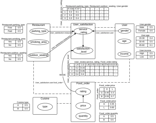
To illustrate these concepts, we use a relational schema of a system where users order foods in restaurants and rate the service of the restaurants. The schema is shown in

Figure 2.1a.

Here, Restaurant, User and Cuisine are entity classes, and User_satisfaction and

Food_order, which represent the relationships Restaurant–User and User–Cuisine

re-spectively, are relationship classes. The attributes User_satisfaction.service_rating,

User.age, User.gender etc. are descriptive attributes whereas User_satisfaction.user_id,

which refers to User.user_id, is a reference slot whose domain and range are the objects of the classes User_satisfaction and User respectively. Restaurant and User_satisfaction objects are directly linked through the reference slot User_satisfaction.resto_id. Note

that Restaurant.resto_id−1 _{is the inverse of User_satisfaction.resto_id and gives all}

User_satisfaction objects corresponding to Restaurant objects. Restaurant objects can

also be indirectly related to User objects through slot chains. For example, the slot

(39)

satisfaction level and/or service rating about the restaurants are available. As there is a many-to-many relationship between the classes Restaurant and User, this slot chain may result into more than one users for a single restaurant. In such case, we need an aggregator (such as average) to summarize (or aggregate) the resulting set. For

in-stance, AVERAGE(User_satisfaction.resto_id−1_{.user_id.age) gives the average age of}

the users who have rated the restaurants. Use of multi-set operators on slot chains can provide interesting results. Let’s take an example of intersection operation between two

slot chains User_satisfaction.resto_id−1_{.user_id and Food_order.resto_id}−1_{.user_id.}

This operation gives those users who have made orders in some restaurants and rated them too. To achieve the same result without the use of multi-set operators, we would need a long slot chain. v

Example 2.2 A relational skeleton for Restaurant-User-Cuisine schema An example of a relational skeleton corresponding to this relational schema is shown in

Figure 2.2. The skeleton has two users, three cuisine, and three restaurants. Here, the

relationships between users, restaurants, and foods are specified but not the descriptive

attributes. Corresponding to this skeleton, Figure2.2c depicts a complete instantiation

of the relational schema. v

2.2.2 Bayesian Networks

A Bayesian network (BN) (Pearl [1988]) is a directed acyclic graph where nodes

correspond to random variables and arcs between nodes represent conditional depen-dencies; lack of an arc between nodes indicates that the variables are conditionally

independent. A BN associates with each random variable Xi a conditional

probabil-ity P (Xi | P ai), where P ai ∈ X is the set of variables that are called the parents

of Xi. BNs achieve compact representation of probability distribution by exploiting

conditional independence properties of random variables. Every node in a BN is

con-ditionally independent of its non-descendants given its parent. This conditional

inde-pendence assumption enables BNsto simplify the joint probability distribution given

by the Chain rule as follows:

P (X1, X2, . . . Xn) =

Y

i

P (Xi | P ai) (2.1)

Example 2.3 Burglary and Earthquake network from Pearl [1988]

Figure 2.3 shows an example of a Bayesian Network adapted from Pearl [1988]. All

random variables in this example take binary states. Each node is associated with a

Conditional Probability Distribution (CPD). The edge between the nodes Earthquake

and Alarm indicates that earthquakes can make the alarm go off. Similarly, if there is an earthquake, it is likely that there will be an announcement on the radio. v

Inference in Bayesian networks

Inference in Bayesian networks generally refers to: finding the probability of a vari-able being in a certain state, given that some of the other varivari-ables are set to certain values; or finding the values of a given set of variables that best explain (in the sense

of the highestMaximum a Posteriori (MAP) probability) why a set of other variables

(40)

2.2. BACKGROUND 17

(a)

(b)

(c)

Figure 2.2 – Instantiations of the relational schema of Figure 2.1a. (a) depicts a relational skeleton as objects and relations between the objects. (b) presents the same skeleton in a relational database. (c) A complete instantiation of the relational schema of Figure 2.1a

(41)

Figure 2.3 – An example of a Bayesian network (Pearl [1988])

be found in the literature. Pearl [1982]’s message passing algorithm is the first one

for performing inference onBNs, and is a basis for many other algorithms (Shafer and

Shenoy [1990]). It calculates marginal distribution for each unobserved node

condi-tioned to any observed nodes. Originally formulated for trees, this algorithm was later

extended to perform inference on polytrees (Kim and Pearl [1983]). These algorithms

are applicable to singly-connected networks only, i.e. the networks that contain only a single path between nodes. Several algorithms exist for probabilistic inference on

multiply connected networks (Lauritzen and Spiegelhalter [1988], Jensen et al. [1990],

Shachter [1986], Sang et al. [2005]). These exact inference algorithms, which

analyti-cally compute theCPDover the variables of interest, are computationally expensive on

large, complexBNs. As a solution, several approximate inference algorithms have been

proposed. These algorithms involve heuristic and stochastic techniques which are not guaranteed to give the correct answer for a given query, but often return values that

are close to the true values (Russell and Norvig [2003]). Henrion [1988]’s probabilistic

logic sampling based on Monte Carlo methods, Jensen et al.[1995]’s block Gibbs

sam-pling, and Weiss [1997]’s loopy belief propagation are some examples of approximate

inference algorithms. In general, BN inference is found to be NP-hard in both the

exact (Cooper [1990]) and approximate (Dagum and Luby[1993]) case.

Learning Bayesian networks

One way to construct a BN is to collect expert knowledge and create the model

based on it. However, this is not feasible all the time as it may be difficult to find experts in the domain of interest. Also, data in the hand may not always be in accordance with

experts’ opinion. Besides, it is very important to be able to construct aBNfrom data in

today’s world, where data are constantly evolving and steadily being modified because such ever-changing data may show different behaviors at different time and hence the model will need to be updated with the changing data. Many algorithms have been

developed in order to learnBNsfrom observed data. Learning aBNinvolves two tasks:

(a) learning parameters (i.e. conditional probabilities), and (b) learning structure (i.e. the DAG structure).

(42)

2.2. BACKGROUND 19

Parameter learning Various statistical and Bayesian methods are available for

learning conditional probabilities inBNsfrom different kinds of data. Maximum

Likeli-hood Estimation (MLE), Expectation Maximization withMLE, MAPand Expectation

a Posteriori (EAP) are some Bayesian approach to parameter learning.

Structure learning Learning aBNstructure is the task of finding aDAG structure

that best represents the probabilistic dependencies existing in the given data.

Exhaus-tive search to find the exact structure of a BN is impossible because the number of

possibleDAG grows exponentially with the number of nodes. Even for 10 nodes, there

are 4.2 × 1018 _possible_DAGs_{. Many techniques have been proposed to learn} _BN

struc-ture. Those techniques can be broadly classified into three families – constraint-based approach, score and search approach, and hybrid approach.

Constraint-based approach In constraint-based approach, aBN is seen as an

independence model and its structure is learned by testing Conditional Independence

(CI)between the variables. Verma and Pearl[1991]’s Inductive Causation (IC),Spirtes

et al.[2000]’s SGS, PC and PC* algorithms fall under this family. They use statistical

tests, such as χ2 and G tests for triples (X, Y, S), where X and Y are variables and S

is a subset of variables, to determine whether X and Y are conditionally independent given S, i.e. X ⊥ Y | S.

Score-and-search approach Also known as score-based methods, this approach

looks for theDAG space in order to maximize a scoring/fitness function that assigns a

score to a state in the search space to see how good a match is made with the sample

data. Score-based algorithms begin with a search space of candidate BN structures,

score each of them, and select the one with the best score. Because the size of the search space grows exponentially with the number of nodes, heuristics are generally applied to explore the search space. Greedy search (GS) is a commonly used heuristic search

method, which performs in the following way: starting from aBNstructure (which can

be empty or not), GS moves to the best-scoring neighbor graph until convergence. GS is said to have converged to the solution when no neighbor graph has better score than the current graph. Intuitively, a graph and its neighbors are almost identical except for small local modifications. Such small local modifications are commonly obtained

by adding an edge, deleting an edge or reverting an edge in the graph (Algorithm 1).

A score-and-search method requires a scoring criterion that gives a good score when a

structure matches the data well. Several scoring functions (such as Bayesian Dirichlet

(BD)(Cooper and Herskovits[1992]),Bayesian Information Criterion (BIC) (Schwarz

[1978]), Akaike Information Criterion (AIC) (Akaike [1970]), Minimum Description

Length (MDL) (Bouckaert [1993]) and Minimum Message Length (MML) (Wallace

et al. [1996]) etc.) have been devised for this purpose. Most scoring functions reward

a better match of the data to the structure and prefer simpler structures. Another desirable property of a scoring function is decomposability, whereby the score of a particular structure can be obtained from the score for each node given its parents.

Hybrid approach The main limitation of score-and-search approach is

scala-bility. For large number of variables, the search space is extremely big, and hence, a good amount of time is needed for examining candidate structures. On the other hand, constraint-based methods offer a fast approach even when there are large num-ber of variables. The outcome of these methods, however, can be adversely affected