Integrated Production and Inventory Control of Assemble-To-Order Systems with Individual Components Demand

HAL Id: tel-00866378

https://tel.archives-ouvertes.fr/tel-00866378

HAL is a multi-disciplinary open access archive for the deposit and dissemination of sci-entific research documents, whether they are pub-lished or not. The documents may come from teaching and research institutions in France or abroad, or from public or private research centers.

L’archive ouverte pluridisciplinaire HAL, est destinée au dépôt et à la diffusion de documents scientifiques de niveau recherche, publiés ou non, émanant des établissements d’enseignement et de recherche français ou étrangers, des laboratoires publics ou privés.

Assemble-To-Order Systems with Individual

Components Demand

Zhi Li

To cite this version:

Zhi Li. Integrated Production and Inventory Control of Assemble-To-Order Systems with Individual Components Demand. Other. Ecole Centrale de Lille, 2013. English. �NNT : 2013ECLI0012�. �tel-00866378�

ECOLE CENTRALE DE LILLE

THESE

présentée en vue d’obtenir le grade de

DOCTEUR

en

Spécialité : Automatique, Génie Informatique, Traitement du Signal et Image

par

Zhi LI

DOCTORAT DELIVRE PAR L’ECOLE CENTRALE DE LILLE

Titre de la thèse:

Commande optimale (en Production et Stock) de

Systèmes Assemble-To-Order (ATO) avec prise en

compte de demandes en composants individuels

Integrated Production and Inventory Control of Assemble-To-Order Systems with Individual Components Demand

Soutenue le 3 septembre 2013 devant le jury d’examen :

Président _{Jean-Louis BOIMOND, Professeur, LISA, Université d’Angers}

Rapporteur _{Alexandre DOLGUI, Professeur,LIMOS, Ecole Nationale Supérieure des}

Mines de Saint-Etienne

Rapporteur _{Bernard GRABOT, Professeur, LGP,}Ecole Nationale d’Ingénieurs de Tarbes Membre _{Jean-Louis BOIMOND, Professeur, LISA, Université d’Angers}

Directeurs de thèse Codirecteurs de thèse

Etienne CRAYE, Professeur, LAGIS, Ecole Centrale Lille

Mohsen ELHAFSI, Professeur, University of California, Riverside

Hervé CAMUS, Maître de Conférences, LAGIS, Ecole Centrale Lille

Thèse préparée dans le Laboratoire d’Automatique, Génie Informatique et Signal, (UMR CNRS 8219) Ecole Doctorale SPI 072 (Lille I, Lille III, Artois, ULCO, UVHC, EC Lille)

À mes parents, à ma sœur,

à toute ma famille, à mes professeurs,

Acknowledgements

This PhD research work has been achieved at Laboratoire d’Automatique, Génie Informatique et Signal (LAGIS) in École Centrale de Lille, with the research teams “Optimisation des Système Logistique (OSL)”, and “Système Tolérants aux Fautes”. I have worked in Ecole Centrale de Lille in France for three years, from September 2010 to September 2013. The PhD thesis is fully supported by the China Scholarship Council (CSC), including the Ecoles-Centrales Intergroup.

I start by thanking all the members of the jury for having accepted to examine this work and for their interests and remarks.

Then my deepest gratitude goes to my supervisors Prof. Etienne CRAYE, Prof. Mohsen

ELHAFSI, and Mr. Hervé CAMUS for having welcomed me and followed me during my

thesis. I would like to thank Prof. Mohsen ELHAFSI, for his professional instructions and suggestions, his personal quality and scientific literacy, and his constant patience and encouragement, that guided me, influenced me and got me through this work. I’d like also to thank Prof. Etienne CRAYE, for his guidance and kindness. His pragmatic and strict attitude toward work set a good example for me in my scientific life. I still remember the words of him “En recherche, il ne faut jamais être ni approximatif, ni superficiel. Avec de la persévérance, de la méthode et de la rigueur, rien n'est impossible.” I’m grateful to my

supervisor Mr. Hervé CAMUS during my three years of thesis, who gives me a great help for

my research work.

Finally, I would like to thank my families and my friends, who support me to overcome any difficulties in the real life.

Villeneuve d’Ascq, France August 16th, 2013

Table of Content

1.2 Optimal Control of ATO Systems ... 13

1.3 General Approach ... 15

1.3.1 Markov Decision Process ... 15

1.3.2 The Value Iteration Algorithm ... 17

1.4 Application of Markov Decision Process in ATO systems ... 18

1.5 Problem Setting ... 22

1.6 Plan of the Thesis ... 23

1.7 Conclusion ... 23

Literature Review ... 25

Chapter 2. 2.1 Make-to-Stock Systems under MDP ... 26

2.2 ATO Systems under Continuous Review ... 28

2.3 ATO Systems under Periodic Review ... 30

2.4 ATO Systems in Continuous Time ... 32

2.5 Conclusion ... 33

ATO System with Individual Components Demand: Lost Sales for Components Chapter 3. and Assembled Product ... 35

3.1 Introduction ... 36

3.2 The Optimal Control Problem ... 37

3.2.2 The Case of Discounted Cost ... 38

3.2.3 Influence of System Parameters ... 55

3.2.4 The Case of Average Cost per Period ... 76

3.3 Numerical Experiments ... 78

3.3.1 Value Iteration Algorithm for Average Cost Criterion. ... 78

3.3.2 The Structure of the Optimal Policy ... 79

3.3.3 The Effect of System Parameters on the Optimal Policy ... 80

3.4 Conclusion ... 86

ATO System with Individual Components Demand: Lost Sales for Components Chapter 4. and Backorders for Assembled Product ... 87

4.1 Introduction ... 88

4.2 The Optimal Control Problem ... 89

4.2.1 Model Formulation and Structure of the Optimal Policy ... 89

4.2.2 The Structure of the Optimal Policy ... 91

4.3 Numerical Study ... 128

4.4 Conclusion ... 139

Heuristic Policies ... 141

Chapter 5. 5.1 Introduction ... 142

5.2 The Case of Lost Sales ... 143

5.2.1 The Optimal Policy ... 143

5.2.2 Three Static Heuristic Policies ... 143

5.2.3 Comparison to the Heuristic Policies ... 147

5.3 The Case of Lost Sales and Backorders ... 153

5.3.1 The Optimal Policy ... 153

5.3.2 Four Static Heuristic Policies ... 154

5.3.3 Comparison to the Heuristic Policies ... 158

5.4 Conclusion ... 162

Conclusions and Future Perspectives ... 163

Résumé Etendu en Français ... 169

List of Figures

Fig. 1.1. Assemble-to-order system ... 12 Fig. 3.1. The structure of the optimal production policy with lost sales ... 82 Fig. 3.2. The structure of the optimal allocation policy with lost sales ... 82

Fig. 3.3 The effect of holding cost h1 on the optimal policy for Component 1 with lost sales

... 83

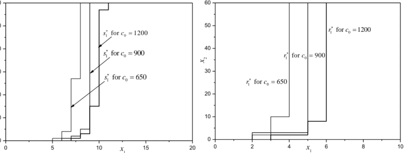
Fig. 3.4. The effect of lost sale cost c0 on the optimal policy for Component 1 with lost sales

... 83

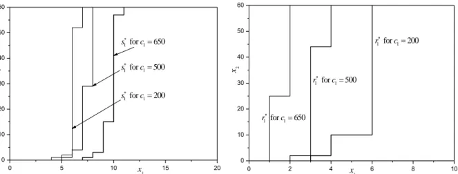
Fig. 3.5. The effect of lost sale cost c1 on the optimal policy for Component 1 with lost sales

... 84

Fig. 3.6. The effect of arrival rate0on the optimal policy for Component 1 with lost sales .. 84

Fig. 3.7. The effect of arrival rate₁on the optimal policy for Component 1 with lost sales... 85

Fig. 3.8. The effect of production rate1on the optimal policy for Component 1 with lost sales

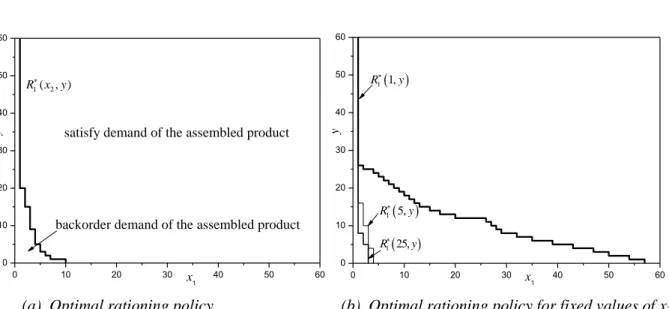
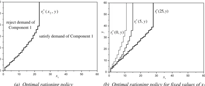
... 85 Fig. 4.1. The optimal production policy for Component 1 with lost sales and backorders ... 131 Fig. 4.2. The optimal production policy for Component 1 with lost sales and backorders ... 133 Fig. 4.3. The optimal production policy for Component 1 with lost sales and backorders ... 134 Fig. 4.4. The optimal allocation policy for demand of the assembled product at Component 1 with lost sales and backorders (b0=10, c1=1000, c2=800) ... 136

Fig. 4.5. The optimal allocation policy for demand of the assembled product at Component 1 with lost sales and backorders (b0=10, c1=100, c2=75) ... 136

Fig. 4.6. The optimal allocation policy for demand of the assembled product at Component 1 with lost sales and backorders (b0=200, c1=100, c2=75) ... 137

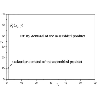
Fig. 4.7. The optimal allocation policy for demand of Component 1 with lost sales and

backorders (b0=10, c1=1000, c2=800) ... 137

Fig. 4.8. The optimal allocation policy for demand of Component 1 with lost sales and

backorders (b0=10, c1=100, c2=75) ... 138

Fig. 4.9. The optimal allocation policy for demand of Component 1 with lost sales and

Fig. 5.1. The effect of the relative load on optimal average cost ... 151

Fig. 5.2. The effect of h1/h2 on the system under Heuristic H1 ... 151

Fig. 5.3. The effect of h1/h2 on the system under Heuristic H3………...151

List of Tables

Table 5.1 Optimal policy versus Heuristic policies with lost sales ... 148 Table 5.2 Optimal policy versus Heuristic policies with lost sales and backorders ... 160

General Introduction

Chapter 1.

The main objective of this work is to study a special case of an assemble-to-order (ATO) manufacturing system that is not only subject to demand for the assembled product but also subject to demand for the individual components. For this purpose, we use a Markov decision process (MDP) framework to formulate the system. In this first chapter, we present a basic knowledge of our work such as the definition of ATO systems, the significant role of optimal control, the principles of the general approach, and the problem setting. Finally, we conclude this chapter with a plan of the thesis.

1.1 Assemble-to-Order Systems

In today’s business environment, with the increasing competitiveness of the global market,

mass customization has become a major objective for many manufacturing companies. This trend has forced companies to adopt a hybrid operations strategy to better deal with a variety of market environments. Towards this end, an assembly system known as ATO, has emerged and became more popular. An ATO system produces multiple components and assembles them into a variety of final products. Demands occur only for the final products, but the system keeps inventory at the component level (Song and Zipkin, 2003). The products can be

assembled from different components while components can be used by different products

(see Fig.1.1). An ATO system simplifies the process of manufacturing. It can be regarded as a manufacturing strategy which allows a product to be made or service to be available to meet the needs of a specific customer order.

ATO systems are characterized by short assembly times and high product variety, which have the advantage of decreasing life cycles of products, meeting diverse customer needs, and saving on total cost. It is an efficient strategy that companies have applied to reengineer their production design. The primary application of the ATO strategy is in the computer assembly industry. For instance, companies such as Dell and IBM benefit from using the ATO strategy. The former is famous for controlling inventory levels of components, and the latter is famous for two-stage server computers. Both of them successfully apply the ATO strategy to enhance their competitive position in the global PC market (Agrawal and Cohen, 2001; Cheng et al., 2005). … 1 … 2 j n … 1 2 m k … … … 1 1 1 2 2 2 j j j n n n Suppliers Components Products Demand for products

…

…

Generally speaking, the ATO strategy is characterized by flexibility and responsiveness, and it is useful for manufacturing companies to secure market share, improve profits and enjoy a competitive advantage.

In this work, we consider an ATO system that produces n components with a single assembled product. Demand from both the product and the components can be satisfied or rejected/backordered. Components are produced one unit at a time on separate production facilities and held in stock incurring a holding cost. We assume exponentially distributed production times, and demand arrives in the system following independent Poisson processes. In our model, since the final assembly time is considerably short, we neglect it. This assumption is reasonable and applied in most ATO systems (see Song and Zipkin, 2003). Due to the possibility of components stock-out, some orders may not be satisfied immediately. The unsatisfied order may be lost or backordered resulting in a penalty cost. In this study we consider two cases: the pure lost sales and the mixed lost sales and backorders. In the pure lost sales case, an order rejected incurs a lost sale cost. Demand from the assemble product has a higher penalty over the demand from the individual components. Due to limited

capacity, it may be desirable to reject a demand from a component even when there is

on-hand inventory of components to satisfy future product demand. In the mixed lost sales and backorders case, a component order rejected incurs a lost sale cost and a product order backordered incurs a backorder cost. In this case, the product demand has no priority over the component demand, thus it may be backordered even when there is stock for all the components to satisfy future component demand. For these two cases, a system manager needs to decide which components to produce, and whether to satisfy an incoming component demand or reject it to reserve stock for future product demand, or whether to satisfy an incoming product demand or backorder it to reserve stock for future component demand. The objective is to minimize the expected total operating costs of the system.

1.2 Optimal Control of ATO Systems

ATO systems can be regarded as a multiple resource allocation that induces load distribution, production planning, requirements fulfilling and inventory assignment. The key challenge in the management of ATO systems resides in the difficulty to coordinate components procurement or production as components procurement or production leadtimes are usually stochastic. This is further compounded by the uncertainty of the demand of the assembled product as well as the individual components, if they are sold separately as spares. Another

challenge for ATO systems is to efficiently manage component inventories and make optimal production and allocation decisions. Because of the complexity of such a system, it would tend to be difficult to control and would be uneconomical to operate. In addition, in many business scenarios where manufacturing companies face limited capacity and shortage

situations that usually cannot be avoided, it is necessary to adopt a feasible strategy to solve

these problems (Akçay, 2002). In this situation, the issue of inventory rationing arises. Because of a limited capacity, it may not be sufficient to produce the total quantity of the order. The manager needs to efficiently manage component inventories and allocation. The problem is how to determine inventory replenishment levels with uncertain demand and how to allocate the components for received demands.

In practice, determining optimal component inventory levels is difficult, especially in a multi-product ATO system. The inventory level of a component at any point in time will depend on the previous allocation decisions. Such decisions depend on the production and consumption of all other components and the demand realizations of all end products. Thus, the problem of determining optimal inventory levels and an allocation policy can be formulated as a dynamic programming with the goal of minimizing the expected long-run system cost. Optimal control is needed to deal with the problem of finding a control policy for a given optimality criterion. For characterizing the structure of optimal policies in the infinite horizon, please refer to the studies by Porteus (1975, 1982), Stidham and Weber (1989).

The main objective of this work is to control an ATO system with demand from both the individual components and the assembled product. In an assembly system, since satisfying a customer order requires multiple available components, the storage of one component delays the fulfillment of the order for product. The optimal control of ATO systems should be correlated across components: the optimal component replenishment policy is applied to the production and the optimal component allocation policy is applied to the inventory. Also, because a customer order requires multiple units of several components, the optimal component allocation policy results in severe computational complexity, especially in the case of multiple demand classes. As mentioned in Ha (1997c), “… as the number of customer classes increases the optimal policy will be difficult to compute because of the curse of dimensionality and will be even more difficult to implement.” This implies that as the state space increases in size, the structure of the policy becomes more complex. Because many dimensions must be taken into account when making allocation decision: the inventory level, the number of backorders as well as the production process. For this reason, characterization

of optimal control policies for ATO systems has been regarded as a challenging problem. Various authors have studied this problem including De Véricourt et al. (2000, 2002), Benjaafar and ElHafsi (2006, 2010), Gayon et al. (2009). They showed that the optimal allocation policy is a multi-level rationing policy. In this work, we adopt a similar approach as these authors to analyze the optimal policy for a more general ATO system.

1.3 General Approach

In this work we study an ATO system. In order to determine a control policy, we formulate the problem an MDP. Then we specify the principle and algorithm in the following.

1.3.1 Markov Decision Process

The models we will study in the next few chapters use the MDP framework. Since demand inter-arrival times and production times are uncertain, randomness is one of the key factors that our models must take into account (see Zipkin 2000, section 7.3). Markov Decision Processes, which are also called stochastic dynamic programs or stochastic control problems, provide a mathematical framework for sequential decision making when outcomes are uncertain.

In a dynamical system the state can change over time. At each decision epoch, a decision maker can choose an action that may influence the future state of the system. Markov decision processes are completely determined by a five-tuple









as follows:

1. S: the set of possible system states.

2. Ax: the set of available actions to the decision maker when the system is in a starting

state x.

3. rt: the cost per unit time. The real-valued function rt (x, a) foraAx denotes the value

at time t of the cost incurred in period t.

4. pt: the transition probability per unit time. The transition probability functionpt





for aAx denotes the system state at the next decision epoch and is determined by





t

p  xa , when action a is chosen in state x, at time t.

the system when action a is chosen in state x, at time t.

At each instant, the transition probability and the cost function depend on the past only through the current state of the system and an action can be selected in that state. This property is called “Markovian”, which has been widely used in inventory control problems. This is because in this setting a Markovian policy is optimal and properties of the optimal policy are simple to carry out and do not vary with time (Puterman 1994, Chapter 1). In order to choose actions, we must follow some policy. We define a policy to be any decision rule for

choosing actions. In other words, a policy is a sequence of decision rules. Thus, the action

chosen by a policy may, for instance, depend on the history of the process up to that state point, or it may be randomized in the sense that it chooses action a with some probability

,

a

p aA. When the policy depends only on the current state of the system, it is called

Markovian policy. In this case, the control function under a policy  can be defined as A in

state S and action a.That is, A( )x is the action selected in x when a policy is employed.

Typically, under a policy  and in state xat time t the decision maker can choose an action a.

The cost generated depends on the state of the system at the next decision epoch. At time t for

a given probability density function ft





cost r_t

 

associated with the starting period. Thus, for a time interval  , at time t , the system

changes to a new state x, which is determined by the distribution p_t





generated over this period is equal to _t( , ) t _s( , )

t

r x a 



state x and the phenomenon is repeated. Because the action is chosen in the present state 

incurs a cost that forces the system to move to a new state. Clearly, a new state is determined

by the previous action choice. When the distribution ft is deterministic, the periods  between

two changes of state are constant and equal, corresponding to the representation of periodic time. The decisions in this case are taken at time t=0,1,2,…, and the specification of the total cost ( , )rt x a over a period is sufficient.

The objective is to determine the optimal policy  that minimizes the discounted cost,

 



where, X is the random process denoting the current state of the system andis the discount

factor (0  1). Since r(X(t)) is the cost generated at time t, it follows that v

 

the expected total discounted cost generated when policy  is applied with the initial state x.

When decisions are made frequently or the discount factor is not assumed





cost case can be considered,

 



where, g

 

is to determine the optimal policy  that minimizes the average cost. The average cost

criterion is simple to implement, because the results of which are independent of the starting state and the discount factor.

In this work, we use these two criteria in our analysis.

1.3.2 The Value Iteration Algorithm

In this sub-section, we consider the computational aspect of MDP. One of the commonly used algorithms in MDP is the value iteration. It is widely used to obtain the optimal policy.

Consider a Markov decision problem





section1.3.1. The objective is to find the optimal policy that minimizes the discounted cost in equation (1.1).

Consider a set F of positive real-valued functions defined on S. Under the previous

hypotheses, there exists an operator T that reflects the dynamic of the system and equation (1.1) can be written as:

vn1

 

 

where,vn

 

 



x , with v0

 

The existence of a Markov policy that achieves the minimum of the discounted cost in (1.1) and the convergence of the n-stage policy and cost function to the infinite-horizon optimal policy and cost follow from the fact that only finitely many controls are considered at each state.

An average cost criterion can also be considered. In this case the average cost per stage, g, and the relative cost in state x, v(x) satisfies,

v

 

 

letting  0 in(1.4) (see Cavazos-Cadena, 1992; Weber and Stidham, 1987):

1. there exists a stationary policy  which achieves a finite average cost g.

2. the number of states in which the holding cost h

 

The value iteration algorithm is the most widely used and best understood algorithm for solving Markov decision problems. It is an easy method to determine the optimal policy. In this work we use the value iteration algorithm, for more details readers can review Puterman (1994, Chapter 8).

1.4 Application of Markov Decision Process in ATO systems

The MDP framework has been used in a wide range of optimization problems. A general application of MDP described in Feinberg and Shwartz (2002, Part III). In this work, we consider an ATO system with limited production capacity, which produces multiple components and assembles them to a signal product. The product is assembled from components only when a customer order is received, and the inventory is kept at the component level. Faced with demands for both, the product and the components, the system manager must determine the optimal policy to minimize the total cost.

In this section, we only present the general characteristics of Markov decision problems. The detailed specification of the models that we study is given in the corresponding chapters.

For this work, we assume a discrete-state setting, and use continuous time by converting to an equivalent discrete time. That is, our ATO system produces n types of components with a single assembled product. The product and the components can meet n+1 demands. For the

pure lost sales case, the state S is a subset of Zn ( is the set of nonnegative integers). In

this case, we define the current state of the system at time t by the vector X(t)=(X1(t),…, Xn(t)),

where Xk(t), k=1,…n, is a nonnegative integer denoting the on-hand inventory for Component

k at time t. For the mixed lost sales and backorders case, the state S is a subset of Zn1.The

current state of the system at time t can be defined by the pair (X(t),Y(t)), where Y(t) is a nonnegative integer denoting the backorder level of the assembled product.

The decisions

For each of the models that we study, the decision maker has to decide which type of components should be produced, and whether to satisfy an incoming component demand or keep stock for future product demand. For instance, in the pure lost sales case: under a policy

 for a starting state x





  



a x  u u w w where u_k 1 means produce Component k (k=1,…,n), u_k 0

means do not produce Component k, w_k 1means satisfy demand from Component k, and

0

k

w  means reject demand from Component k, w₀ 1 means satisfy demand from the

assembled product, and w₀ 0 means reject demand from the assembled product. In the

mixed lost sales and backorders case: under a policy  for a starting state

  



the decision maker takes actions a

  

 _{   }

 x ...,w_n



Component k to stock, u_k 2 means produce Component k to reduce the backorder level of

the assembled product, and u_k 0 means do not produce Component k, w_k 1means satisfy

demand from Component k, and w_k 1 means reject demand from Component k, w₀ 1

means satisfy demand from the assembled product, and w₀ 0 means backorder demand

from the assembled product.

The cost structure

The related costs of our system are incurred from two sources: the cost of holding inventory and the cost of backordering. We assume the costs are linear, such as r_t

   

and r_t

   

 

functions, h_k( ) denotes the holding cost of Component k per unit per unit time, b₀( ) denotes

the backorder cost of the assembled product per unit per unit time.

The transition probabilities of the state

Since production times and demand inter-arrival times are stochastic, we focus on these two

uncertain sources: production times are exponentially distributed with mean 1 _k, demands

take place continuously over time according to independent Poisson processes with rate _k

(for Component k)and ₀ (for the assembled product), respectively.

When the transition times are identically one, it is a Markov decision process, and in general case, it is called a semi-Markov decision process (see Ross 1969, Chapter 7). In the optimal control of exponential queuing systems, we use a semi-Markov decision process. That because a sequential decision process for which the times between transitions are random. In this work, we consider the following two cases:

Pure lost sales case

As mentioned above, in the pure lost sales case the current state of the system at time t can be

described by the vector X( )t 











x the decision maker takes the action a. Let e





vector of ones and ek the kth unit vector of dimension n. In the state x, if the decision maker

chooses the action to produce one unit of Component k, the state will transfer to the state x+ek

with thetransition rate_k. If she takes the action to satisfy one unit order from the product,the

state will transfer to the state x-ewith thetransition rate₀, or decides to satisfy one unit order

from Component k,the state will transfer to the state x-ekwith thearrival ratek.

Mixed lost sales and backorders case:

In the backorders case, the current state of the system at time t can be described as the pair









  



case is more complex than the pure lost sales. Because besides considering the on-hand inventory x, the backorder level y from the assembled product must be considered. In this

which would incur two different results: produce one unit Component k to stock, the state will

transfer to the state (x+ek,y); or produce one unit Component k to reduce one unit backorder

from the assembled product, the state will transfer to the state





maker takes the action with transition rate ₀, which would lead to satisfy one unit order of

the assembled product, the state will transfer to the state (x-e,y); or to backorder one unit demand of the assembled product, the state will transfer to the state (x, y+1). Similarly, with the rate _k, a transition occurs after time t, the next state may be (x-ek, y). Clearly, the

distribution of time between two instants of decision depends only on the action specified by the control policy applied by the decision maker. Following Lippman (1975), we uniformize the transition rate by defining the uniform rate  _ln_0_l n_k1_k . However, the next state of the system depends on the transition probability. We will discuss them for two cases, pure lost sales and mixed lost sales and backorders:

Pure lost sales case:

In state x, an action a is selected. If the next state is x, the system state at the next decision

epoch is determined by the transition probability p





follows:  1 ( , ) , , k k u k p a  I   x    x x = x e  1 0  0 0, and 1 ( , ) n , , k k x w p a  I         x x x = x e ( , ) _{ 0, and 1}, , k k k k x w p a  I    x  x x e x

Mixed lost sales and backorders case:

If an action a is selected in state (x,y), the next state is

 

   

 x x  , which can be generated as follows:



   



  





   



 







   



  





   



  



where I_{ d} is the indicator function (I_{ d} 1 if d is true, and I_{ d} 0,otherwise).

The optimal policy

Because the system is memoryless, a Markov policy is optimal. In this study, we formulate the problem as continuous-time MDP. That is, the decisions can be made at any time. Applications in inventory control are modeled by allowing action choice at random times in

infinite horizon. The core problem of MDP is to find a policy  in the state S that minimizes

the expected discounted (average) cost. For all possible states S, we will find the optimal cost

function v and use it to determine the optimal policies.

1.5 Problem Setting

In this work, we study an ATO system where we consider demands for both the individual components and assembled product. That is, the product is assembled from multiple components and the components stocked in advance of demand. These products will be used to satisfy the potential orders that arrive later. Components are produced one unit at a time on separate production facilities and held in stock, which incur a holding cost. In addition, both production times and customer inter-arrival times are stochastic. Due to the possibility of shortages, if an order is not satisfied immediately it incurs a lost sale cost or a backorder cost that depends on whether or not the customer is willing to wait for his order. Therefore, the task of the decision maker is to decide whether to satisfy an incoming demand or reject (backorder) it, reserving stock for the future demand from a more valuable type. At the same time, the decision maker also decides which component is needed to produce, if needed, whether to produce it to stock or to produce it to reduce the backorders from a particular demand. The objective is to minimize operating costs while maintaining order fulfillment. In general, this kind of problem can be regarded as a dynamic problem and a decision support tool is needed. In our work, we study the ATO system from an operations’ perspective. We

use a Markov decision process framework to determine an optimal policy under both the total expected discounted cost and the average cost per period criteria. We characterize the structure of an optimal policy. We carry out numerical experiments to analyze the structure of the optimal policies. We also offer some managerial insights to control the assembly systems. Furthermore, we show that the optimal production policy is a state-dependent base-stock policy, and the optimal inventory allocation policy is a state-dependent rationing policy. More importantly, we show that the optimal policies are highly sensitive to various system parameters such as the holding and the lost sale/ backorder costs, the demand and production rates.

1.6 Plan of the Thesis

The rest of this thesis is organized as follows:

Chapter 2 provides a brief review of the related literature to this work.

Chapter 3 aims at characterizing the optimal policy of the ATO system with lost sales. We determine the structure of the optimal policy and investigate the impact of different parameters on the optimal policy.

Chapter 4 aims at characterizing the optimal policy of the ATO system with lost sales and backorders. We characterize the optimal production policy and the optimal allocation policy for the components.

In Chapter 5, we develop several heuristic policies for the pure lost sales case and the mixed lost sales and backorders case. For each case, we compare the performance of the heuristics with the optimal policies, and then we find some more efficient heuristics.

Finally, the general conclusion sums up the main results obtained and the perspectives describes some future researches of this work.

1.7 Conclusion

ATO systems are successful strategies that have become increasingly popular in manufacturing. This work studies an ATO system that produces multiple components with a single assembled product. Such a system deals with both product and components demands. In this chapter, we introduced an overview of ATO systems, the basic principles of the

policy. We also presented the application of MDP in ATO systems, based on which we formulate our problem.

Literature Review

Chapter 2.

This chapter provides a brief review of the literature related to ATO systems. As mentioned in Chapter 1, the optimal control of ATO systems consist of two decisions: component replenishment and component allocation. These decision problems can be formulated as a single-product or multi- product models, and a single- period or multi-period models. For a comprehensive literature review, we can refer to one classical paper by Song and Zipkin (2003). It covers modeling issues and analytical methods, and a general formulation of ATO systems. From this overview, the literature review on ATO can be classified into the following four categories, which we will discuss in details.

2.1 Make-to-Stock Systems under MDP

Make-to-stock (MTS) systems are manufacturing strategies to manage inventory. In MTS system, products are stocked in advance according to a forecast of customer demand. Because the manager faces a joint production-control and inventory allocation problem, MTS systems can also be called production-inventory systems. A challenging problem in such systems is the dynamic allocation of inventory to different demand classes. This gives rise to an inventory rationing problem which has been widely studied in the literature.

The earlier work on inventory management and production scheduling dates back to Zheng and Zipkin (1990), who studied the optimal control of allocation problem. A simple Markovian behavior is assumed, the problem can be modeled as rationing a fixed production capacity to multiple identical products. More importantly, the authors proposed longest-queue policy and argued that it is always optimal to serve the longest queue under independent base stock policies.

Ha (1997, 2000) pointed out that for a two-dimension state space MTS production system, the optimal production policy is the dynamic “hedging point” policy, and the optimal allocation policy is a “state-dependent rationing” policy. Ha (1997a) is the first to consider rationing in the context of an MTS system. He modeled the system as a single server, single product, M/M/1 make-to-stock queue with multiple demand classes and lost sales. The optimal policy is characterized by a sequence of monotone threshold levels. Under this threshold rationing policy, each class has a rationing threshold below which the demand from that class cannot be satisfied. The system reserves inventory for the orders from the high- priority classes. Ha (1997b) studied hedging point policy with dynamic scheduling problem. By considering single server, two products, make-to-stock queue with backorders, he showed that the optimal rationing policy is of the “switching curve” type. Furthermore, two production switching cures have been obtained: one curve determines when and which product can be produced, and the other curve determines in which region the production can be stopped. In a similar MTS system, Ha (1997c) considered the backorders case but with single product and two priority demand classes. He characterized the optimal production and inventory rationing policies by a single monotone witching curve. He showed that the optimal production policy is of base-stock type and the optimal rationing policy is determined by rationing level, which is decreasing in the number of the low-priority class backorders. In a later article, Ha (2000) extended the results of his work (1997c) to Erlang distributed production times in lost sales

case. Using work storage as a state variable, he indicated that the optimal production policy can be characterized by a critical work storage level. Gayon et al. (2009) analyzed a similar

system as Ha (2000) for an M/Ek/1 make-to-stock queue with multiple classes and they

provided a formulation in the case of backorders and examined the effects of optimal policies under different operating conditions: with and without salvage market value. They showed that the optimal allocation policy with a salvage market is work-storage rationing policy that is characterized by n work-storage rationing thresholds corresponding to n demand classes. Without a salvage market value, they showed that the modified work-storage rationing policy is optimal and is determined by the base-stock level.

De Véricourt et al. (2000, 2002) also considered “hedging point” policies and developed further characterization of the optimal switching curve for the backorders case. The backorders case is more difficult to analyze than the lost-sales case when there are multiple demand classes. One of the major reasons is that backorders of the different demand classes increase dimensionality of the system. Therefore, the analysis is more complex. De Véricourt et al. (2000) showed that in a two-part types production system, it is optimal to produce the expensive item if it has the higher backorder cost. De Véricourt et al. (2002) studied a capacitated supply system with multiple demand classes. By decomposing the problem into n-dimensional control problems and (n-1)-n-dimensional sub-problem, the optimal policy can be characterized simply by fixed threshold values. In the same vein, De Véricourt et al. (2001) evaluated the benefits of different optimal rationing policies: first come first service (FCFS), strict priority policy (SP) and the multilevel rationing policy (ML), and showed that the ML policy performs better than the other two policies. Gayon et al. (2009) characterized the optimal policy for a production-inventory system with multiple customer classes and imperfect advance demand information (ADI). They showed that in lost sales setting the suppliers benefit more from ADI than customers.

Unlike the pure backorder system or pure lost sales system, Benjaafar et al. (2010a) addressed a more general model, taking into account both features lost sales and backorders. Moreover, this paper initiated a study of the structure of the optimal policy in MTS system with both backorders and lost sales. In their case, the backorder and lost sale costs are similarly ordered. Under this assumption, for each class the optimal production/allocation policy can be characterized as a threshold policy. Benjaafar et al. (2010b) studied a production-inventory system with customer impatience. The unsatisfied customer is either lost or backordered. The

depends on the exponentially distributed patience times. That means the customers will wait for an amount of time for fulfilling orders; otherwise, they cancel their orders. In particular, this paper showed that optimal policy base-stock level is non-increasing in the upper bound on the number of backorders, while the optimal policy rationing level is non-decreasing in that. In the same vein, Benjaafar and Elhafsi (2012) studied a two-customer class system: patient and impatient customers. The unsatisfied orders from the patient class can be backordered while the unsatisfied orders from the impatient class can be rejected. The optimal policy can be described by two threshold functions where inventory allocation is not static, which depends on the backorder level of the patient customer class.

There are several studies in the literature that consider production-inventory systems with transshipment/inventory sharing. Benjaafar et al. (2004) discussed the problem of inventory rationing in a system with multiple products and multiple production facilities. Zhao et al. (2005) considered a two-location inventory-sharing system. They used a (S,K) policy, namely base-stock and rationing policy in a decentralized setting. Zhao et al. (2008) also considered a two-location system, while the transshipments can happen in both demand arrivals and production completions. They proved that for each location the optimal production policy is a hedging point policy and the optimal demand filling policy is a state-dependent policy.

There is also a stream of literature that considers the stock rationing problem with batch demand. Huang and Iravani (2008) provided a non-unitary demand system and focused on the problem of rationing quantity. They showed that the order size can affect the benefit of the optimal stock rationing policy. Xu et al. (2010) extended the model of Huang and Iravani (2008) to the multiple-class, batch demand system, where the batch demand can be partially accepted. They showed that the optimal policy is characterized by multiple rationing levels. ElHafsi et al. (2010) studied an integrated production inventory system with multiple non-unitary demand classes. It is assumed that both production times and order inter-arrival times follow the Erlang distributions. They showed that the demand size variability can significantly affect the operating cost of the system.

2.2 ATO Systems under Continuous Review

In contrast to MTS systems, which keep inventory at the end-product level, ATO systems keep inventory at the component level. When the customer order is received, the components can be assembled immediately and delivered to the customer. To our knowledge, most papers

address continuous review models and develop heuristic policies to evaluate or optimize the decisions. In this stream, Song (1998) studied the performance measures for a base-stock system with Poisson demand and constant replenishment leadtimes. She showed that in a multi-item inventory model the order fill rate can be obtained by a series convolution of the batch size distribution and Poisson distribution. Xu (1999; 2001, Chapter 11) studied the effect of arrival correlation on the performance of the ATO system, and discussed how the system responds to different arrival correlations. Gallien and Wein (2001) considered ATO systems with a single-item MTS environment. But in their model, the setting is based on a Poisson demand and an arbitrary distributed processing times. Associated with non-identically stochastic lead times and infinite capacity, the authors developed a simple and effective control policy for an ATO system. That is the structure of the optimal policy is entirely determined by the longest procurement delay and its differences with the other procurement delays. Similar system studied by Song and Yao (2002), who proposed upper and lower bounds for the backorders in a single product case. They showed that it is optimal to keep higher base-stock levels for components with longer mean lead times (and lower unit costs). Lu and Song (2005) formulated an unconstrained cost-minimization model in multiple- product assembly system with order-based backorder costs. They developed an algorithm to approximate the optimal base-stock level. Under the assumption that demands follow a batch Poisson process, Lu et al. (2005) focused on the expected backorder for each product. They solved the optimization problem by minimizing a weighted average of backorders over all products. Later, Lu (2006) extended the model (Lu et al., 2005) to product, multi-component ATO system with general random batch demands. He focused on the average backorder of the system, based on which he developed a new methodology for performance analysis of the system. Zhao (2009) also considered a multi-product and multi-component ATO system with batch ordering. He analyzed and evaluated the impact of the split orders/non-split orders on system performance. Hoen et al. (2011) studied a multiple end-products system with lost sales and deterministic leadtimes. They devised an approximate method for estimating the order fill rates.

Another line of research on ATO systems is base-stock policies with fixed base-stock levels. Song et al. (1999) studied the impact of limited capacity on ATO systems and evaluated performance of base stock policies with stochastic leadtimes. They showed that exact performance measures are a result of multidimensional Markov chains. Glasserman and Wang (1998) considered a system consisting of multiple types of demand, which take place

according to batch Poisson processes. The inventory of each component is controlled by a base-stock policy, and the replenishment leadtimes are i.i.d. (independent and identically distributed) random variables. They focused on a target fill rate and studied the trade-off

between inventory levels and delivery leadtimes. Dayanik et al. (2003) considered an ATO

system consisting of multiple components and multiple products. They developed lower bounds to estimate the order fill rates for the system. Plambeck and Ward (2007) introduced a separation principle for a class of ATO systems with expediting. They demonstrated that the multidimensional assembly control problem can be separated into a series of single-item inventory control problems. Ko et al. (2011) studied a single product, multiple-component production system under a base-stock policy. They provided explicit approximations of the lead times distributions, from which the base-stock levels can be calculated.

For a more general multi-product ATO system: non-identical production system, where the products differ in characteristics. Lu et al. (2010) focused on the W-, N-, M-system and assumed identical component leadtmes. They used a stochastic program to obtain optimal inventory strategy. Dogru et al. (2010) discussed W-system with identical component lead times and proposed a simple priority allocation policy. Under this environment, Lu et.al. (2012) studied an ATO N-system with non-identical leadtimes. This is the special case of W-system. Under the symmetric structure, the optimal component allocation decision is a no-holdback (NHB) rule and the optimal production decision is a coordinated base-stock (CBS) rule; under the asymmetric structure, the optimal policies depend on the effect of cost asymmetry. Reiman and Wang (2012) considered the model of Dogru et al. (2010), while with non-identical lead times. They developed a multi-stage stochastic program and established a lower bound on the inventory cost of the system, based on which they also discussed the replenishment policy and the allocation policy.

2.3 ATO Systems under Periodic Review

For periodic review models, faced with multi-customer classes and integer-valued correlated random variable in each period, a static threshold production/allocation policy has been considered. In general, as mentioned in Chiang (2003) “…earlier periodic review models, however, have focused on the situation which supply lead times are a multiple of a review period. Such models could be regarded as an approximation of continuous review models, as the review periods can be modeled as small”. The earlier literature about this related problem is studied by Cohen et al.(1988) who investigated two demand classes (the emergency

demand and the normal demand) inventory system in a (s,S) policy with lost sales. Assuming the emergency demand has higher priority than the normal demand, the former can be satisfied first. In this setting, a strict priority rule is used for the allocation policy. Furthermore, authors developed and evaluated an efficient and effective solution heuristic for solving the service-constrained optimization problem. Later, Rosling (1989) considered an infinite horizon model with random demands multi-echelon inventory system. Under an assumption of zero setup cost, he showed that a balanced base-stock policy is optimal for multistage assembly systems. Chen (2000) extended this equivalence between assembly and serial systems to the batch-ordering case. He showed that the batch ordering policy is an optimal policy for multi-echelon systems. Cheng et al. (2000) considered a configure-to-order (CTO) system. Such a system takes the ATO concept one step further, and then the customers can select the personalized set of components that assembled to the end product. They used a lower bound on the order fill rate of each product to investigate the optimal inventory-service tradeoff. Karaarslan et al. (2013) considered a single item, two-component system with backorders under two different policies: a pure base-stock policy and a balanced base-stock policy. They showed that the balanced base-stock policy works better under low service levels, low holding cost ratio, and high demand uncertainty. Otherwise, the pure base-stock policy performs well.

Turning to the study of single-period ATO systems, Fu et al. (2006) analyzed the policy of pre-stocking components and a single product ATO system with uncertain demand and limited assembly capacity. They examined the effect of varying component leadtimes on the available assembly capacity. Xiao et al. (2010a) also considered the similar system as Fu et al. (2006), but focused on an ATO system with both uncertain demand and uncertain assembly capacity. By considering assembly-in-advance operations, the authors adopted a profit-maximization model and investigated the optimal production and inventory decisions. Xiao et al. (2010b) extended their study to a two-product production system with two types of uncertain demand. They studied the impact of the uncertain demand patterns on the optimal stocking and allocating decisions.

We found also several review articles on different inventory allocation policies. See, for example: Zhang (1997) considered an assembly system with multiple productions and dependent demands. He proposed a fixed-priority policy with stock commitment for allocating component stocks. Hausman et al. (1998) studied joint demand fulfillment

studied assembly type production systems with demand uncertainty under a fair-share policy. Several results are used to determine the optimal base-stock policy. Akçay and Xu (2004) considered a multi-component and multi-product ATO system under the independent order-based policy. Duran et al. (2007) focused on limited production capacity inventory system with multi-period time horizon. They considered two customer classes differentiated by their priority level, and showed that a (S, R, B) base-stock policy is optimal, where S is the order-up-to quantity, R is the reserve-order-up-to amount, and B is the backlog-order-up-to amount. Feng et al. (2010) worked on a multi-item inventory system under the (r,nQ) policy, where r is the recorder point, nQ is the order size. They showed that the joint inventory positions of the system are stationary, independent and uniformly distributed.

2.4 ATO Systems in Continuous Time

In this section we discuss ATO systems that are managed/operated in continuous time. In this case, the problem is formulated using MDP. In this research branch, an initial view of the optimal control of a system with multiple components on multiple production facilities, and multiple demand classes is given by Benjaafar and ElHafsi (2006), who studied an ATO system consisting of n products assembled from a subset of m distinct components. By assuming that the manager is faced with multiple demand classes, they analyze the optimal production and inventory allocation policies of such system. Unlike the fixed allocation policy, the optimal allocation policies are dependent on the on-hand inventory of the other components. The optimal inventory policy for one component can be described as a state-dependent policy that depends on the on-hand inventory levels of all other components. In this article, although the authors considered a special case of an ATO system, it still can be viewed as a classic one. Because also under continuous review, compared with the other literatures (mentioned in section 2.2) which focus on performance evaluation of heuristic policies, this work determines the optimal production policy.

ElHafsi et al. (2008) also considered an n- product and m-component ATO system where the products have a modular nested design. They showed that the optimal production policy is a base-stock policy and the optimal inventory allocation policy is a multi-level rationing policy. Finally, ElHafsi (2009) studied an ATO system subject to non-unitary multiple demand classes. The author argued that comparing to the effect of order size variability, the optimal average cost rate is more sensitive to the order size. More recently, Benjaafar et al. (2011) discussed a multiple stages, multiple demand classes assembly system with batch production

and batch demand. By considering different items can be produced in different batch sizes, they characterized the optimal policy. In particular, the optimal production quantity for each component and the optimal number of satisfied requirements for each demand class would also be determined.

In this work, we study a continuous time ATO system, and share several common features in the above literature of ATO system under continuous time. That is, the assumption of exponential production time and Poisson process demand. The current work is most closely related to that of Benjaafar and ElHafsi (2006). Similar to their model, we study an ATO system with a single product assembled from n components. However, in our system we consider two types of demand: demand of the assembled product and demand of the individual components, and discuss the demands with the pure lost sales (see Li, 2013a) and the mixed lost sales and backorders (see Li, 2013b). Based on which, we study the optimal control policy.

2.5 Conclusion

We provided a brief overview of the literature involved in this work, which can be classified into four categories: make-to-stock systems under MDP, ATO systems under continuous review, ATO systems under periodic review, and ATO systems in continuous time. Our work is more related to the literature on ATO systems in continuous time. In this line of research, we study the model that deals with two types of demand ATO system: the assembled product demand and the individual components demand. To our knowledge, there is little literature in this area. We hope that the research presented in this work also enriches the current literature on ATO systems with individual components demand.

ATO System with Individual

Chapter 3.

Components Demand: Lost Sales for Components

and Assembled Product

We consider the demand during shortage period as completely lost. In this chapter, we assume that if demand cannot be fulfilled immediately it is lost for both the assembled product as well as the individual components. We propose a dynamic programming model in order to determine the optimal control policy of such a system. The system deals with a single product which is assembled from multiple components. The system faces demand not only from the assembled product but also from the individual components. To determine the optimal operating policy, we formulate the problem using an MDP methodology and using two optimality criteria: discounted cost and average cost per period. Furthermore, we determine the structure of the optimal policy and investigate the impact of different parameters on the optimal policy. We are also interested in the effect of system parameters on the optimal policy. We test the system with a wide range of system parameters and show that the optimal base-stock and rationing levels are sensitive to system parameters

The outline of this chapter is as follows: we start with an introduction in section 3.1. In section 3.2, we formulate the optimal control problem with lost sales and characterize its optimal policy under the discounted cost case. Then we extend our model to the average cost case. In section 3.3, we adopt the average cost criterion in numerical experiments, and use the iteration algorithm to calculate the optimal policy. Based on numerical results, we analyze the structure of the optimal policy. Finally, we conclude this chapter in section 3.4.

3.1 Introduction

This chapter considers an ATO system with a single product assembled from n components. Each component is produced ahead of demand one unit at a time on an independent production facility. Unit held in inventory incurs a unit holding cost. Demand from both the product and the components can be either satisfied or rejected. Demand for the assembled product can be satisfied only if all components are in stock. We assume that demand for the assembled product has a higher priority over demand for the individual components. In this situation, a system manager may need to reject a demand from a component and save the inventory for future assembled product demand. At the same time, a system manager needs to decide when to produce a certain component and when not to produce it. We also assume exponentially distributed production times, and demands arrive to the system according to independent Poisson processes. We assume that the assembly time is instantaneous and there are no setup costs and setup times for production. Our assumption of negligible assembly time is supported by most of the literature on ATO systems.

A system manager must make two types of decisions: one regarding component production and the other regarding inventory allocation. The objective is to determine the optimal control policy that minimizes the expected operating costs of the system. In general, this kind of problem can be regarded as a dynamic problem and a decision support tool is needed. In our study, the problem can be formulated as an MDP resulting in Markovian policies. We show that the optimal production policy is characterized by state-dependent base-stock levels. That is, a component is produced when the on-hand inventory is below the base-stock level, and not be produced otherwise. Moreover, the base-stock level is non-decreasing in the on-hand inventory level of other components. We show that the optimal inventory allocation policy is a rationing policy. An order from a component is satisfied only if its on-hand inventory level is above a certain rationing level. The rationing level for each component is also non-decreasing in the on-hand inventory levels of other components. This is an interesting property since both the base-stock and the rationing levels are non-decreasing in the on-hand inventory level of other components. This result is quite different from the ones in (Benjaafar and ElHafsi 2006, ElHafsi et al. 2008). In our system we discuss two types of demand: demand of the assembled product and demand of the individual components. Benjaafar and ElHafsi 2006 studied a single product ATO system, ElHafsi et al. 2008 studied a nested-multiple-product ATO system, where they consider one type of demand that can only be from