Combinatorial Optimization for Fast Scaffolding

(1)

HAL Id: hal-01251290

https://hal.inria.fr/hal-01251290

Submitted on 6 Jan 2016

HAL is a multi-disciplinary open access archive for the deposit and dissemination of sci-entific research documents, whether they are pub-lished or not. The documents may come from teaching and research institutions in France or abroad, or from public or private research centers.

L’archive ouverte pluridisciplinaire HAL, est destinée au dépôt et à la diffusion de documents scientifiques de niveau recherche, publiés ou non, émanant des établissements d’enseignement et de recherche français ou étrangers, des laboratoires publics ou privés.

Combinatorial Optimization for Fast Scaffolding

Ivaylo Petrov

To cite this version:

Ivaylo Petrov. Combinatorial Optimization for Fast Scaffolding. Bioinformatics [q-bio.QM]. 2014. �hal-01251290�

(2)

Research Master Thesis

Combinatorial Optimization for Fast Scaffolding

Author: Ivaylo Petrov Supervisor: Rumen Andonov Antonio Mucherino GenScale

(3)

Abstract

In recent years the topic of genome assembly has become a focus of a number of research publications. Even though many researchers have focused on the assembly of large genomes such as humans’, the assembly of much shorter genomes such as those of the chloroplast and the mitochondria organelles is yet not fully resolved. The available methods do not consider all the available information. They are also unable to provide more than one possible solution for the scaffolding problem. We tackle those unresolved situations by using exact methods that consider all the available information. Our methods are also capable of producing all the optimal solutions. Therefore, we believe our approach will be very beneficial for the biologists.

1 Introduction

1.1 Context

For a long time researchers have been fascinated with the diversity of living beings on Earth, the study of the differences and the similarities among species. With the advent of technologies, more and more characteristics of species have been documented for many living organisms. It is now known that, inside each living organism, there is a number of building units, called cells. Moreover, in each cell, there is a molecule, called DNA1. It consists of a sequence of nucleotides and encodes the genetic instructions necessary for the development and the behavior of all living organisms. Therefore, understanding the development and the behavior of living beings, is strictly related to understanding this molecule. The challenge is in the decoding of the information contained in the DNA. Several issues need to be overcome during the decoding process.

One of these issues concerns the sequence of nucleotides of the DNA. That sequence is different for each individual, differing from person to person, exception made for identical twins. Although the DNA is unique for every individual, some parts of it are common for all the people. The same rules apply to all the other species as well. Another critical issue is the following. Once the DNA molecule has been sequenced for a single individual, how to decode and understand the information that it contains?

This is somehow similar to the situation where a compiled version of a software tool in an unknown (let’s say alien) programming language is available. In order to analyze such a software tool, any scientist would greatly benefit from having the source code of the program, even if they cannot really read and understand it. They could, however, find similarities in the code that lead to similarities in the software behavior, i.e. in its execution. The situation with the study of the DNA is quite similar. Scientists believe, that if they have the structure of some DNA molecule, it will be much easier for them to try to understand it.

When working with a DNA molecule, one of the main difficulties is the lack of a technology that can read the structure of an entire DNA molecule in one shot. That is why, subsequences of nucleotides are actually read from the DNA. To this end, each subsequence is named read.

Many technologies, capable to provide “reads”, have emerged. The difference between them is not only given by the size of the reads they provide, but also by the price for each DNA sequencing and the way the reading positions are chosen. For example, for newer technologies, the reading positions are chosen at random. This leads to a need of high coverage2 in order all the parts of the genome to have good chances of being represented. As for the difference in the read sizes, Sanger sequencing reads have sizes ranging from 500 to 1000 bases. They are quite smaller than the size of the human genome (which is around 3,234.83 mega bases), but still few times bigger than the reads of most of the newer technologies. As stated in El-Metwally et al. [2013] there is also a difference in the number of errors that are inserted during the sequencing. The difference in the price and the throughput, however, makes the newer technologies much more preferable than the old ones in a variety of situations.

Nevertheless, this gives rise to a new issue to overcome: how to gather all those small pieces together. There are two ways to approach this problem. If some reference sequence is available then, it is possible to try to position the pieces onto the reference sequence, while allowing some small changes. Although this approach has the advantage of being simple and fast, it does not

1

There are some exceptions like a mature red blood cell.

2

(5)

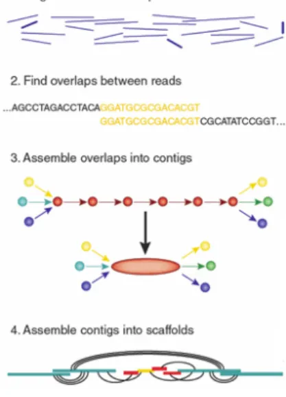
allow to obtain a genome that is completely different from the template. Furthermore, the choice of the reference genomes, in case there is more than one, affects the result and therefore this approach cannot be very accurate. For these reasons, a second approach was proposed. It consists in assembling the reads on the basis of overlaps between pairs of reads. The approach is called de novo genome assembly. An image representing the whole process for producing scaffolds can be seen in Figure 1.

A naive way to approach the problem of whole-genome shotgun (WGS) de novo assembly3 is by trying each piece with every other and see if they match well together. After that, some heuristics are used to estimate the best matching. Even though this approach was not very efficient, it was used for some time. In Pevzner et al. [2001] was proposed an approach that makes use of the de Bruijn graph. For more information about this approach, please refer to the article Pevzner et al.

[2001].

It turned out, however, that the short reads are not sufficient to represent more complex parts of the genome, including some partial repetitions. These repetitions are long parts that come at multiple positions in the genome and are longer than the read size. In order to represent these complex parts, some additional information was added to the output of the sequencing of some of the new technologies - mated read-pairs4. With this new information, the DNA structure can be represented more correctly, allowing the creation of better tools for assembling genomes.

Figure 1: De novo genome assembly

1.2 Assembling strategies

The process of assembling the small reads of DNA into bigger parts can be divided into at least two phases. The first one creates contigs from the read, most commonly using some overlapping criteria. Contigs are gapless sequences of nucleotides. The second phase is the scaffolding, or the process

3

This is the so far described process of assembling small reads from different parts of the genome, usually with very high coverage that tries to compensate the randomness of the sequenced places

4

That is a pair of read for which we have additional information about their relative orientation and distance between them. In the literature they are also referred to as read pairs

(6)

of producing the best possible scaffolds (according to some criteria and some information that is presented). Scaffolds are generally sequences of contigs and gaps, the sizes of which are known. Often, contigs are oriented into scaffolds and ordered linearly in such a way which minimizes the number of unsatisfied scaffolding constraints (as defined in Gritsenko et al. [2012]). Scaffolding constraints might be, for example, relative position and relative orientation of pairs of contigs, inferred from the mated read-pairs.

1.3 Scaffolding

In the scientific literature, there is currently no formal and widely accepted definition for the Scaffolding problem. In an informal way, it is the inferring of the positions and the orientation of contigs along the genome, based on some possibly inconsistent information. Most often that information consists of mated read-pairs, but it can include other sources of information as well. In section 3, we will attempt to provide a formal definition of the problem.

The Scaffolding problem is the last step in the genome assembly process. Kececioglu and Myers

[1995] showed that the problem is NP-hard. The main difficulty comes from fact that the available data are inherently noisy. Because of that, Scaffolding algorithms should be conceived for handling such situations.

In this report we will first describe the work that has already been done in section 2. Next we will provide a formal definition of the scaffolding problem in section 3. After that, we will present four approaches for solving it for the chloroplast and the mitochondria organelles in section 4. We will discuss the strengths and the weaknesses of each of them in section 5. Next, we will point some of the possible improvements of the presented methods in section 6. And finally, we will conclude in section 7.

2 Related work

The topic of contig scaffolding is a well studied one. A number of previous attempts have been made to provide a good solution for it. They propose several methods which have a number of positive and negative properties. A short discussion of their strengths and weaknesses will be provided shortly. One of the most common problems is the use of unreliable heuristics that might result in solution very different from the optimal one. Another widespread problem is the use of small portion of the information that is available to the scaffolder. Some of the existing methods aim to solve the problem exactly, but their performance is not always very good in regard of speed or accuracy, according to independent studies (see Hunt et al. [2014]).

• Velvet Zerbino et al. [2009] is a very fast algorithm. It uses a simple and fast heuristics to order the contigs in the most probable way, according to the provided information. The accuracy of this approach is generally not as good as that of the others. It also does not use the information about the contig coverage.

• SOAPdenovoLi et al.[2010] is another algorithm that tries to use not very complex heuris-tics in order to scaffold big genomes. The focus of this approach is more on speed than on accuracy. One of the contributions of this approach is its capability to use multiple data sources with multiple insert sizes. On the other hand, the solutions that it provides are not very accurate as it does not aim to fully analyze the provided data.

(7)

the problem exactly. After that article, there have been some other ideas about how to solve the problem exactly. However, according to a number of independent studies (seeHunt et al.

[2014]), they are not having the same accuracy as that approach. This is partially due to the fact that the SOPRA algorithm tries to produce correct scaffolds, rather than long ones. It also tends to run slower than a number of its competitors. In the article about SOPRA

(see Dayarian et al. [2010]) it is also proposed to use partitioning of the graph in order for

every partition to be solved independently. More about the partitioning will be presented in section 4.2. This idea has been employed in other approaches as well.

When the size of the component is not very big, an exact approach, based on Dynamic Programming, is used. Otherwise, a heuristic method, based on Simulated Annealing, is employed.

The SOPRA method also tries to solve the problem of overlapping of contigs exactly, by trying to find the minimum contradicting information that needs to be removed.

To sum up, this approach tries to greatly improve the quality of the scaffolds, that it produces, by better using the provided information. Sometimes the method is very slow, even though it uses some heuristics in order to improve its runtime. It also does not aim to use the contig coverage5.

• MIPSalmela et al.[2011] was inspired by the idea of finding exact solution to the scaffolding problem. The difference between this approach and the previous one is that, here, the authors propose to bundle a number of edges together, so that the structure of the resulting graph is more compact. Moreover, MIP uses heuristics to delete a number of edges, that are considered as not trust-worthy. That way, the resulting graph can be partitioned into small components which can be solved exactly using mixed integer programming techniques.

Although this technique is quite faster compared to SOPRA and tries to solve the problem exactly, it tends to produce less accurate results. It shares the same attitude to contig coverage as SOPRA - it disregards this information. Due to the time improvement, however, a number of people prefer it to SOPRADayarian et al.[2010].

• Opera Gao et al. [2011] is another method that tries to solve the problem exactly. The differences between Opera and the previous two methods are in the better grouping of the edges6 and in the lack of any heuristics. In the paper it is explained that due to the sparse nature of most of the scaffolding graphs, it is possible to achieve an acceptable runtime for most cases even without the use of heuristics. It is also proved that if some of the properties of the graph are bounded, it is possible to solve the problem exactly in polynomial time. Despite being exact, this method sometimes produces less accurate results than some of its competitors, according to Hunt et al. [2014]. It also does not use the contig coverage information and it can not provide more than one possible solution.

• In the GRASSGritsenko et al.[2012] paper, the authors formulate the scaffolding problem in terms of a set of scaffolding constraints that might have different weights. That is a significant difference with all the previously described methods, where the only constraints that were used are coming from the mated read-pairs.

The problem that this approach is trying to solve is to find the most probable scaffold, that would lead to the observation that was made when the data was read.

Expectation-5

From the text of the article it seems like this is the case. Some other articles also suggest that.

6

In the previous method, all the edges that suggest the same orientation between a pair of contigs are grouped together. In this method only similar edges are grouped together.

(8)

maximization approach is applied for achieving this goal.

Despite providing some good ideas, this approach can not be expected to exactly solve the problem. Another drawback of this approach is that it does not consider contig coverage. It also tries to find just a single optimal solution, which might not be the most useful result for the biologists.

To sum up, the most common problems of the already provided approaches are the use of heuristics, the consideration of a part of the input data and not the whole input data, the attempt to provide only one possible solution. In the current document we will resolve all of the above problems by using exact algorithms that will consider all the available information7.

3 Definition of the scaffolding problem

Let Γ be the input set of contigs and let l(c) and cov(c) be such that for any contig c, c ∈ Γ, l(c) gives the length in number of nucleotides of the contig while cov(c) gives the number of times the contig c is expected to occur in the genome. Let N =X

c∈Γ

cov(c).

Let O = {F, R} represent the possible orientations of each of the contigs, where F stands for forward orientation and R stands for reverse orientation. Let for better notation assume that F = R, R = F and (o1, o2) = (o1, o2), o1, o2 ∈ O.

Let P be the set of the read pairs that are given. Let orient : P → O2 gives the relative orientation of the contigs. We should note that in the general case, there might be several read pairs for each couple of contigs (c1, c2), c1, c2 ∈ Γ. Let dist : P → N provide the distance between

the contigs for each of the read pairs. The distance is measured in number of nucleotide bases. Note that it can be negative, which means that the two contigs have some overlapping. This can be a result of big k-mers’ size. Even when there is some overlapping between two contigs, if it is smaller than the size of the k-mers that was used to produce the contigs, then it is not possible to combine the two contigs together. That is when negative distances occur.

Let contigs : P → Γ2 be a function that for each read pair p gives the pair of contigs that it connects. Let head : P → Γ and tail : P → Γ provide the first and the second contig of contigs(p) for any given p ∈ P .

Then the scaffolding problem can be defined as follows - find a triplet of functions

(rank, pos, or) :    rank : {1, . . . , N } → Γ pos : {1, . . . , N } → N or : {1, . . . , N } → O (1)

Where the function rank gives a mapping between the numbers from 1 to N and contig occur-rences. For a given number it provides the contig that is associated with that number. The number does not provide information about the ordering of the contig. That information is provided by the pos function, which is an injective function. That function provides information about the position where each contig occurrence is located on an axis. This can be used to calculate the distances between the contigs. For each given contig occurrence for contig c, that is associated with the number i (rank(i) = c), pos(i) gives the position of the center of the contig on an axis, where

7

Some of the approaches that we will provide lack some of the noted characteristics, but it is possible to use their solutions to help the other approaches.

(9)

that contig occurrence should be positioned. The or function provides orientation of each contig occurrence.

If dist match : P → N provides a score for the degree to which the distance of every read pair is satisfied. That is to say that it provides the best score between any contig occurrences of the contigs of the read pair. A possible definition of dist match would be the following:

dist match(p) :        1

if ∃i, j ∈ {1, . . . , N }, such that rank(i) = head(p) and rank(j) = tail(p) and

|pos(i) − pos(j)| − dist(p) −l(head(p)) + l(tail(p)) 2 ≈ 0 0 otherwise (2) And if or match : P → {0, 1} is a function that for each read pair p provides whether the orientation of any contig occurrences of the contigs of p, according to or, is contradicting to the one suggested by p or not. It has a value of 0 if the orientation is contradicting for all of them and 1 otherwise.

or match(p) :   

1 if ∃i, j ∈ {1, . . . , N }, such that rank(i) = head(p) and rank(j) = tail(p) and (or(i), or(j)) = orient(p) or (or(j), or(i)) = orient(p)

0 otherwise

(3) Then the following conditions have to be true for the functions rank, pos and or.

• ∀c ∈ Γ : n j ∈ {1, . . . , N } : rank(j) = c o ≤ cov(c)

• Find the pos and or functions which maximize the following function:

X

p∈P

dist match(p) × or match(p) (4)

The scaffolding problem can be explained then as finding the best positions and orientations of the contigs occurrences, so that a maximal number of mated read-pairs are satisfied. Depending on the choice of dist match function one can have different models for the scaffolding problem that can be solved as optimization problems.

4 Proposed models

In this section we describe four different approaches to the scaffolding problem. They are aiming to provide robust way for scaffolding of the genomes of chloroplast organelles and mitochondria organelles. In this special case of the scaffolding problem, it is realistic to expect that the result will be just one scaffold and not a number of scaffolds, as the coverage that the sequencing machines provide is big enough. Despite that, this problem is not sufficiently well studied. All the approaches that are targeting this part of the scaffolding problem use heuristics. Furthermore, at least most of them do not use the coverage information that is provided by the contig assemblers. Another feature that our approaches aim to improve is the number of possible solutions. In practice it is known that several distinct solutions are possible for the scaffoldings of the genomes of those organelles. All the existing approaches, to the best of our knowledge, aim to provide just one

(10)

optimal solution. We, on the other hand, provide all the optimal ones, as that will be useful for the biologies.

For validating the solutions that we provide, we use examples, for which the answers are known. That way we can verify that some of our solutions are the same as the provided one. All the other optimal solutions are equally possible ones, according to our formulation of the problem. In regards of the provided data any of the optimal solution has the same probability to be correct as the provided one.

The examples are created, using data that is provided to GenScale by some of its partners. The data consists of reads, mated read-pairs and the expected final result. Using that raw data, we first filter it8. After that, the reads are combined into contigs, using a tool created by GenScale. Next, we map the mated read-pairs information onto the contigs. After that, using the expected final genome, we create the expected solution in terms of contigs positions and orientations. That is the data our approaches are using. It would be relatively easy to add support for fasta and fastq files to our methods, but this is still not done.

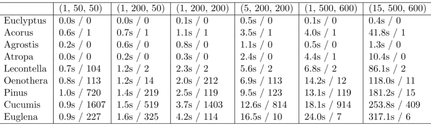
We have provided implementations for all of the approaches that we will describe. They have been designed with the idea of being compared, thus we have being trying to give them the same scoring function. For some of them we use slightly modified scoring function during the construction of the solution, as otherwise we would have to also modify the models. Still, we have implemented ways to score all the methods using exactly the same function, which provides us with some pos-sibility to compare the performance of those different approaches. Those comparisons can be seen in Table 4.

Three of the models that we are going to describe are exact. That means they are trying to find the best possible solution by the criteria that we have set. It is possible to limit the time of search for some of them, which might result in finding suboptimal solution. Some of the approaches have also the possibility to provide all the best solution and not just one of them. We believe that this will be very beneficial for the biologists.

One of the approaches is heuristic, which means that not only we can not guarantee that it always finds the best solution, but we can not find all the solutions that are believed to be optimal, using it. It will be described, nevertheless, as it can also be used together with some of the other approaches in order to improve their performance. This is done as the heuristic results are used to provide information about the expected score of the optimal solution as well as some information about its structure. It is then easy to use that information for the Branch and Prune approach. When the size of the problem is big enough the heuristic approach runs considerably faster than the other approaches. That is why it is rational to use it to try to improve the runtime of the other methods, by providing them with some information about some at least locally best solution.

Before we present the heuristic approach in section 4.5, we will first describe the graph repre-sentation that we chose in section 4.1. After that we will give information about possible ways to decrease the size of the problem that we are trying to solve in section 4.2. Then a Linear Program-ming model will be described in section 4.3. Next a description of a Branch and Prune model will be provided in section 4.4. After that, the heuristic Genetic Algorithm model will be presented in section 4.5. Finally the Distance Based Approach will be described in section 4.6.

8

(11)

v1 v2

Forward direction

v1 v2

Reverse direction

Figure 2: On the left part of the figure is presented the read pair (v1, v2) → (F, R) with forward

direction from left to right. On the right part of the figure the same read pair can be seen, but looked in the opposite direction and as a consequence the orientations of the contigs are reversed. It is equivalent to having a read pair (v2, v1) → (F, R).

4.1 Graph representation

The graph representation that was chosen is used in almost all the models. We aim to stick with the same representation, so that the descriptions are easier to understand and the comparisons are fare. Here is a description of the representation itself.

• Nodes are built using the contigs and the expected number of times they should be met in the genome. For each time a contig is expected to be presented in the genome, two nodes are created - one for each of the possible orientations of the contig. We assume without loss of generality that one of them represents the reading of the contig in forward direction and the other - in reverse direction. The direction will be important when the read pair information is added to the graph.

• Directed edges are built to connect the nodes that represent contigs that are connected with read pairs. In order two contigs to be connected, their orientations should be consistent with the orientation suggested by the read pair. In other words if we have a read pair that connects (c1, c2), the nodes for c1 and c2 will be connected with a directed edge, but for example c1

and c2 will not be connected.

• Directed edges are built for all read pairs when they are looked in reverse direction, i.e. swapping forward and reverse in the orientation of the contigs and swapping the places of the contig numbers - the first becomes the second and vice versa (see Figure 2).

To make things clear, let us consider a simple example. Lets say that we have three contigs → {c₁, c2, c3}. For c1 we have two occurrences in the genome, while for the other contigs we have

only one. For those contigs we have the following mated read-pairs: (c1, c2) → (F, F ), (c1, c2) →

(F, R), (c1, c3) → (F, F ), (c2, c3) → (R, F ). Here we have omitted the information about the

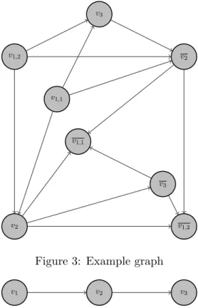
dis-tance between the contigs in order to simplify the graph. Otherwise it will be presented on the edges. The resulting graph can be see in Figure 3. There each contig is represented as a few vertices - two for each occurrence of the contig. The notation is as follows: the nodes for each contig i are called v_i[,k]. The second index, if present, means the occurrence of the contig. For example the second occurrence of c1 is represented as v1,2. Throughout this document to signify a reverse

ori-entation of a contig occurrences, we use overline. For example v1,2 denotes the reverse orientation

of the contig 1 in its second occurrence. The absence of overline signifies forward orientation. To sum up, the nodes are {v1,1, v1,1, v1,2, v1,2, v2, v2, v3, v3} and the edges are

(12)

v1,1 v1,1 v1,2 v1,2 v2 v2 v3 v3

Figure 3: Example graph

v1 v2 v3

Figure 4: A node, v2, with exactly one predecessor and exactly one successor.

{(v_1,1, v2), (v2, v1,1), (v1,1, v2), (v2, v1,1), (v1,1, v3), (v3, v1,1), (v1,2, v2), (v2, v1,2), (v1,2, v2), (v2, v1,2), (v1,2, v3), (v3, v1,2), (v2, v3), (v3, v2)} 4.2 Graph reformatting

In this section some techniques to decrease the size of the graph in order to improve the performance of the scaffolder are presented. They do not change the nature of the problem that is being solved as well as they do not change the solutions of the problem. Similar techniques are used in a number of previous works, including Dayarian et al. [2010]; Salmela et al. [2011], but in those cases the covering of the contigs have not been taken into account to the best of our knowledge. The addition of the covering slightly changes the problem.

The first optimization is to detect the cases where one contig has exactly one predecessor and one successor (see Figure 4). In that case if the coverage for the three contigs are cov(v1), cov(v2), cov(v3)

(13)

v1 v2&v3

Figure 5: A node, v2, with exactly one predecessor and exactly one successor.

and without loss of generality let us assume that cov(v1) >= cov(v3), and if cov(v2) = cov(v3), then

we can delete the v2 contig and the v3 contig as well as its two edges on the figure and substitute

them with a new artificial contig and a new edge between v1and that artificial contig (see Figure 5).

The rational behind this is that we want to use every contig the number of times it is indicated by the data, if that is possible. By making this substitution we do not change whether it is possible or not to use the contigs the required number of times. To illustrate that let us consider the following scenario: in order to go to the v2 contig we should always visit v3 and each time we visit

v3, we should visit v2, as otherwise we will be unable to visit v2the required number of times. Then

it is clear that we can merge the two contigs into one artificial contig, for which some of the bases that form it are unknown (this is not allowed for the normal contigs).

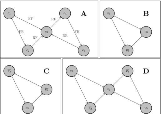
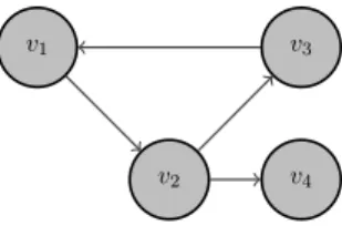
Another technique, that can be applied, is the graph partitioning. It is already studied in a number of other articles (see Dayarian et al.[2010];Salmela et al.[2011]). The idea that is used in those works is to find articulation points (seeWestbrook and Tarjan [1992] for ideas how to do it efficiently) of the graph and partition the graph based on those articulation points. After that for every partition the problem should be solved independently and the results should be recombined. This approach is applicable if the structure of the genome is linear and not circular. Then the orientation and ordering of each of the contigs in one component depends only on the orientation of the articulation vertex. To better illustrate this, we will describe an example.

There are five contigs each of which is met only once. That forms ten vertices:

{v₁, v1, v2, v2, v3, v3, v4, v4, v5, v5}

The mated read-pairs between them are: {(v1, v2), (v1, v3), (v2, v3), (v3, v4), (v5, v3), (v4, v5)}.

A visualization of this example can be seen in Figure 6A, where instead of writing v1, v1 we

have used c1 in order to simplify the figure. In that figure it can be seen that the graph can be

partitioned into two parts with respect to c3. In Figure 6B the solution for the first partition is

provided. In Figure 6C a solution for the second partition is given. It can be seen that although the orientation of contig c3 for those two solutions is different, they can still be combined to form

the global solution as shown in Figure 6D. This is done using the reverse of the original solution for the second part. As it was already described, each read pair can be used as if it is looked from left to right or as if ti is looked from right to left. That is what is used here.

The problem that we are focused on, however, is for ordering contigs of chloroplast genome. It differs from the case on that picture by shape of its genome - it is not linear, but circular. As a consequence it is not true that if we remove any one vertex in the graph, the graph will no longer be connected. As a result there will be no parts that can be solved separately. Furthermore, even if we try to remove two vertices, we will be unable to combine the solutions for the two parts. That is the case as they might contain contradicting information about the orientation of some contig as they have not one, but two vertices in common. For that reason the technique with taking the reverse of every contig occurrence in the subgraph is inapplicable.

Another possible technique to reduce the size of the graph and as a result to improve the performance of the algorithms is presented in Gao et al. [2011]; Salmela et al. [2011]. The idea is

(14)

c1 c2 c3 c4 c5

A

FR FF RF RF FR RR v1 v2 v3

B

v3 v4 v5

C

v1 v2 v3 v4 v5

D

Figure 6: In figure A the structure of the graph is given. After that it is divided at the vertex v3. The solutions for each of the sub problems are presented in B and C respectively. For those

two solutions the contig c3 has different orientations. This is solved in figure D where the reverse

solution of the one in C is used.

to put similar mated read-pairs as a single edge. In Salmela et al.[2011] all the mated read-pairs that suggest the same orientation between a pair of contigs are put together. As a result the size of the graph is significantly reduced. The drawback of this realization of the provided idea is that the mated read-pairs might have significantly different lengths. Then it is not easy to decide how to resolve this. For that reason inGao et al.[2011] the authors propose only mated read-pairs with similar lengths to be put together.

Another thing to notice about this approach is that the support, or the number of times a mated read-pair was presented in the input data, should be preserved. Otherwise incorrect solutions might be produced.

4.3 Maximum Weighted path approach

In this section we are going to present our first method for solving the scaffolding problem. It is somewhat different from the others in that it does not use the distances between the contigs. Despite the fact that it does not use that very important piece of information, this method can produce very nice results, especially in combination with some parts of the other methods.

The objective here is to place linearly the contigs in a way that maximizes the number of read pairs whose orientation corroborates the orientation of the contigs that are associated with them. This is not as strong requirement as when the distances are also used. As a result this approach might produce a number of suboptimal solutions according to the optimization function used for the other approaches. Despite that, it is relatively easy to filter the suboptimal solutions afterwards, at least for the experiments that we have made.

(15)

The main motivation of the model is to be simple and to be able to find contradictions in the input data (i.e. to detect that no linear allocation of contigs exist that satisfies the given read pairs’ orientations and coverage). When the data is not controversial it tends to find all the optimal solutions very quickly.

Method description

This approach can be seen as a filling of a table M of size [2 × N, N ]. To each contig from the input we associate two rows in the table - one row for each orientation of the contig. The column i corresponds to the ith contigs in the solution and can be seen as the ith step in the graph walk. The problem then is to find a path in the graph, such that the below set of constraints are satisfied: • Each node is visited at most once, meaning that the sum for each row in the table is at most

one9.

• Each of the nodes have just one orientation.

• The orientations of the nodes does not contradict the constraints imposed by the read pairs. This is at least partially enforced by the construction of the graph.

• On each step exactly one contig is visited.

The optimal walk is such that maximizes the read pairs, for which the contigs that they connect, are having the orientation that is suggested by the read pair.

In other words, the sum in each column k (

2N

X

i=1

Mi,k) and in each two row that represent the

same contig occurrence j, j + 1 (

N

X

i=1

Mj,i+ Mj+1,i) should be equal to one, meaning that at each

step we take, we use exactly one contig occurrence and that this contig occurrence is not used in any of the previous steps.

We have also added the constraints that in order Mi,j to be 1, some of the neighbours of

that node should have a value of 1 on the previous step. This can be implemented as follows: ∀k, l : Ml,k ≤

X

w∈neighbours(l)

Mw,k+1. As we know the sum can be either 0 or 1. This statement says

that if Ml,k was 1 on the previous step, then some of its neighbours should also have value 1 on the

next step.

In order to keep track of the mated read-pairs that are satisfied, we introduce additional variables fi that represent whether some node is used. That information is used after that to verify that

the orientations of both contigs of the read pair are the expected ones. If this is the case another variable has value of 1, otherwise its value is 0. The sum of those variables is used as function that we need to maximize.

Mathematically the above constraints can be written as:

for each column k ∈ {1, . . . , N } :

2N

X

i=1

Mi,k = 1 (5)

for each row i ∈ {1, . . . , 2N } : fi = N

X

k=1

Mi,k ≤ 1 (6)

9

(16)

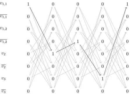
v1,1 v1,1 v1,2 v1,2 v2 v2 v3 v3 0 0 0 0 0 0 0 1 0 0 0 0 0 0 0 1 0 0 0 0 0 0 0 1 0 0 0 0 0 0 0 1 0 0 0 0 0 0 0 1

Figure 7: A walk in the example graph as performed by the algorithm

∀i ∈ {1, 3 . . . , 2N − 1} : fi+ fi+1= 1 (7)

∀k ∈ {1, . . . , N }, l ∈ {1, . . . , 2N } : Ml,k ≤

X

w∈neighbours(l)

Mw,k+1. (8)

for each read pair (i, j) : fi+ fj ≤ 1 + yi,j (9)

maxX

p∈P

yp (10)

In Figure 7 it is possible to see the way the Maximum Weighted path algorithm works. The ex-ample that is considered is as follows. The contigs in it are {c1,1, c1,2, c2, c3}. For them the following

read pairs are available: (v1,1, v2), (v1,1, v3), (v1,1,, v2), (v1,2, v2), (v1,2, v3), (v1,2,, v2), (v2, v3), (v3, v1,1), (v3, v1,2).

The black arrows show the actual path that the algorithm found and the light gray ones show the other edges of the graph, that were not used by the algorithm.

As it can be seen, the node v1 is used three times, even though it has coverage of 2. This is

done in this way as most of the genomes of the chloroplast are cyclic and as a consequence the first and the last contig in the walk should coincide.

Implementation details

In practice, if some information is missing or just incorrect, it is possible that there will be no path that goes through all the contigs. If that is the case, the approach that we described above will be unable to find any solution as it expects the data to be correct. This expectation allows it to run very quickly. For the biologists, however, this is not always very useful, as the data that they have might contain errors. If the algorithm does not produce any solution the biologists will have no

(17)

v1

v2

v3

Figure 8: An example where one of the contigs can not be part of the path. In this situation, although it might be possible to position all the contigs, the algorithm detects a possible problem: a missing information about the distance between v1 and v2. It will substitute the contig v2 with

the artificial contig.

idea what is the problem. In order to improve that, we introduce an artificial contig. It is special in the following ways. First of all, it is connected with all other contigs. This is to solve the cases similar to the one in Figure 8. In this figure that represents a simplified version of the available information. It is impossible to find a path that goes through all the contigs for this example. For that reason the artificial contig will take the place of contig v2. As it is connected to all the other

contigs, it will be possible to create a path like v1, < artif icial contig >, v3, v4, v1.

Another thing that is specific for this contig is that it can be used any number of times. In order to restrict the number of uses of this contig, the objective function has a term that penalize the use by some constant times the number of uses of the artificial contig.

maxX

p∈P

lpyp (11)

where lp = 1 if p is one of the provided read pairs and lp= −10000 if p is one of the artificially

added pairs.

As a result, this artificial contig is used the minimum possible number of times. When it is used, it replaces a contig occurrence. This provides clues to the biologists as of which part of the genome might contain errors or missing information. It also enables our algorithm to finish successfully.

4.4 Branch and Prune

4.4.1 Overview of Branch and Prune algorithms

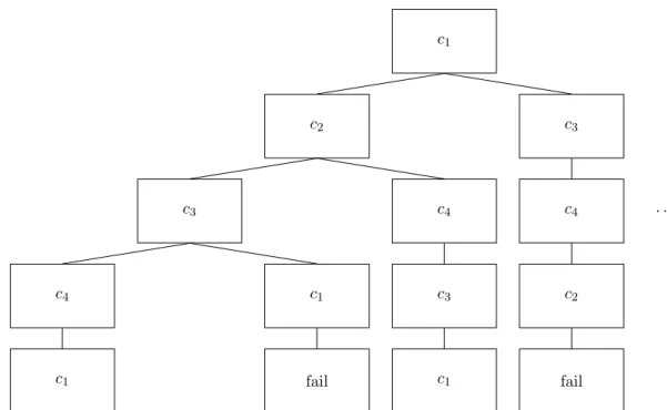
In the literature Branch and Prune is a general algorithmic technique for finding optimal solutions for a vast class of optimization problems (see Van Hentenryck et al. [1997]). The idea of the algorithmic technique is to enumerate all the possible solutions of the problem and while doing so to prune some subsets of candidate solutions based on evidence for sub optimality. While the algorithm enumerates the possible solutions, it build a search tree. In that search tree the nodes represent variables and every path from the root to some leaf node represents a possible solution.

The Branch and Prune approach is one of the most natural ones, even though in general it is less efficient than some other approaches. The lack of good efficiency is a result of the way the algorithm

(18)

operates. It does not aim to use some specific properties of the problem that would allow it to consider just a small portion of the possible solutions in the general case. That is why in a number of situations there are more efficient algorithms. In a variety of other situations, however, it is not that inefficient. For example, if there are very good pruning conditions that eliminate sufficiently large amount of the solutions, the speed can improve dramatically. In theory, it might be possible for some problems to prune all the suboptimal solutions when you start to build them. This will result in a very efficient algorithm. If there are no strong pruning conditions, this approach tends to be less efficient than some of the other possible ones.

The branch and Prune approach have a similar philosophy to that of the Branch and Bound approach, however, for the Branch and Prune one there is no good way to bound the score of a class of solutions. For that reason it is not always easy to limit the number of explored solutions.

One of the good properties of that approach is that a way to find all the optimal solutions can be easily implemented. It does not require significant additional work both in terms of implementation effort and in terms of computational time. Another one is that it is guaranteed to find the optimal solution for the problem it is exploring.

4.4.2 Our implementation of a Branch and Prune Algorithm

Our implementation of the Branch and Prune algorithmic technique is as follows. We build a path through the graph of consecutive nodes. The idea is to find a path from one node back to itself, that goes to all the other nodes. The last point we made was not entirely correct, as for each contig occurrence we have two nodes in the graph. During the building of the path only one of every such two nodes can and should be visited. See Figure 9 for an example of partial search tree that the Branch and Prune algorithm explores.

As there might be a large number of paths in the graph and some of them will not be able to produce optimal solution, we apply methods to detect as much of those situations, as possible and we prune the search tree accordingly.

For that purpose we use two techniques to detect when a partial solution will not lead to a real optimal solution. The first technique that we use aims to detect if from the current partial solution it will be possible to visit all the contig occurrences that are still unvisited. We also verify that it will be possible to go to the first node in the path from the current configuration as the structure of the genome is supposed to be circular.

The other pruning criterion is the score of the solution. It is possible to find a limit of a score of a partial solution, using the fact that if all the contig occurrences are already positioned (they are part of the path), then it is possible to verify if the read pairs that they participate in are satisfied, given that the other contig in that read pair is also already positioned. As a result the score can only get worse with the addition of new nodes to the path as additional read pairs are verified and they might not be satisfied. In this manner it is possible to decide that some parts of the search tree can not lead to a solution that is at least as good as the current best one. Consequentially, they can safely be pruned.

That process explains what can be done to improve the runtime of the algorithm. It does not, however, provide details about the time of execution of each of those verifications. As they are not very fast (O(n0+ m) for the reachability check, where n0 is the number of remaining vertices and m is the number of edges). It is then not very hard to notice that it is not practical to run the verifications on each step as that will make the algorithm slower. For that reason we have decided to do the following things. We run the verifications every v step, where v is a parameter

(19)

c1 c2 c3 c4 c1 c1 fail c4 c3 c1 c3 c4 c2 fail . . .

Figure 9: An example of part of the search tree that the Branch and Prune algorithm will explore for a graph with contigs c1, c2, c3, c4 and read pairs (c1, c2), (c2, c3), (c1, c3),

(c3, c4), (c4, c1), (c4, c2), (c4, c3). We have skipped the orientation and the distances of the read

pairs to simplify the example

of the program. This does not seem very optimal as well, as it might lead to a big number of branches in which we descend and run the verifications, despite the fact that there has been a step that guarantees sub optimality, which has been taken right after the last verification. In order to improve this, we also have dynamic testing. It means that under some circumstances, we decide that it is necessary to run the verifications and we do it. If those circumstances are not present, we do not run the verifications.

The circumstances that were mentioned in the previous paragraph are as follows. If while the algorithm explores a branch, it goes to a configuration where it is not possible to add more nodes to the path or the reachability condition in not satisfied, then the reachability condition is marked as broken and that information is propagated to the previous step of the algorithm. In that case a reachability verification is run for the parent of the current configuration. This is done in order to ensure that all the branches of the search tree, that start from the parent configuration, have chances to produce a solution. In this situation we don’t know if the problem with the reachability was introduced with the last ”step”, or, for example, with the step that lead to it.

Something similar can be applied for the score as well. If at some point the verification or the score of a possible solution suggest that the score of the current path can not be optimal, some of the nodes along the way are verified. The strategy for the verifications is the same as the one described in the previous paragraph.

So far we have described how those checks propagate backwards. In other words how the information that there might be a need of a check is provided to the parent of some partial solution. But sometimes there are situations in which it is clear that such checks are not necessary. For

(20)

v1

v2

v3

v4

Figure 10: In we are at v2, we can not know that there is no path through v4. It is afterwards,

when we are at v3 or v4 that we can notice that.

example, if some of the branches of the current partial solution leads to a solution, it is clear that it is not necessary to check if it can lead to an optimal score. The same strategy can be used for the reachability tests as well.

Also, if some of the children of the current configuration performed some of the checks and the result was not pruning, then the parent does not need to perform that check again.

Despite the fact that the pruning logic in our implementation can eliminate the need to consider a vast number of candidate solutions, it seems that there is more that can be done. This is particularly true when we consider if all the unvisited vertices in some partial solution can be visited in the path. Currently we only verify that each of those vertices is reachable from the current one. This, however, do not guarantee that there will be a path that will be able to visit all of them. As it can be seen in Figure 10, it is impossible to find a path through v4 that goes to

all the other nodes as well. Our verification can not detect that. It will claim that it is possible to construct a solution. This leads us to the question whether it is possible to do something better. The graph can be simplified so that it contains only the vertices that are not visited and the last visited vertex. The task now is to find a path in the graph that goes exactly once through the vertices of the graph, staring from a particular node in the graph and ending in another particular one. This is a special case of Hamilton Path Problem. This problem is well studied and it is proven to be NP-complete not only in the general case, but also for some more specific cases like directed planar graphs with indegree and outdegree at most two (seeGarey et al. [1974] andPlesnik[1979]). The next question that comes to mind is whether we can use some heuristics. There are some very good heuristics that run in O(n3) time. They tend to find a Hamilton path in the graph most of the time when there is one. There are, however, cases when there exists such Hamilton Path in the graph, but the heuristics can not find it. In order to be usable for our algorithm, the heuristic should only make errors of type 1 - false positive. In other words it can say there is a Hamilton Path when there is none, but it can not say that there is no Hamilton Path when there is one. Unfortunately such heuristic can not exist, because in order to say that there is a Hamilton Path, it should find one such path. Then it would be possible in polynomial time to verify whether the provided path has the required properties. If this is not the case, the result of the invocation of the algorithm will be corrected. As a result all the errors that this hypothetical algorithm will make can be corrected in polynomial time. Its runtime is also polynomial, which means that this algorithm can be modified to find a Hamilton Path in polynomial time. This is impossible, and consequentially such algorithm does not exist. As a result there is no obvious way to improve this part of the pruning in our implementation of the Branch And Prune Algorithm.

In order to minimize the calculation during each of the verifications, a number of caches are used, so that no calculation is performed multiple times. According to our experiments this as well as the use of a custom linked list implementation greatly improves the runtime.

(21)

Another technique that we use in order to improve the runtime of that algorithm is to run a number of threads. The number of threads that is to be used is left to the user to choose. The best results are expected to be achieved when using number of threads close to two times the number of processing cores on the CPU (for CPUs with hyper-threading).

The work is distributed to the threads in the following way. First all the threads receive a part of the search tree to explore. After that each thread can receive additional subtrees to explore, if it finishes exploring the one it is assigned. That way the effectiveness is around 350% for 4 threads, which we consider a good improvement.

As it was already noted, the Branch and Prune method has a number of good properties. It, however, do not work for all possible graph configurations. It is possible that some information about distance between pairs of contigs is missing. If the missing information is between contigs that have to be put one next to the other in the final solution, this method will fail. For that reason we add artificial contigs. They have a length of zero and their only purpose is to provide connection between real contigs. As it is not known in the beginning where those connections will be needed, the artificial contigs are connected to every other contig. Apart from those differences from the real contigs, the artificial contigs are almost the same as the others. They can be used only once, etc.

As we don’t want them to influence the score of the solutions, the links between them and the other contigs do not have a fixed length. The length is determined when the length of the read pairs to the neighboring contigs are considered. It is the most probable one. In other words, the one that is most often met, if there is more than one possible. We use that value to calculate the number of violated read pairs afterwards.

In the Maximum Weighted path approach there are again artificial contigs, but they are not exactly the same as those presented here. The difference is that there they replace the use of a read contig, whereas here this is not the case. Another difference is that here the number of artificial contigs should be explicitly given, for example by the user, whereas in the Maximum Weighted path approach this is not necessary.

4.5 Genetic algorithm

4.5.1 Overview of genetic algorithms

The idea of trying to simulate evolution of individuals that describe some problem in order to find the best solution dates from the 1950s, but it gained more popularity during the late 1960s and early 1970s as an optimization technique. One of the important materials on this topic was Fogel

et al.[1966]. That was the first book that tried to study in a great depth the evolutionary approach

to artificial intelligence.

In the 1970s the work of John Holland greatly contributed toward the popularization of the genetic algorithms (seeHolland [1975]) as reliable optimization techniques.

As a consequence of the research, a number of different variations of genetic algorithms are now present. They all have a number of things in common. First of all, the possible solutions of the problem are presented as individuals of some population. The problem then is to find the fittest of those individuals, where the fitness of an individual is determined by a function.

Quite often such approaches are used for optimization problems and in those cases the fitness is related to the optimization problem. Let us take an example to illustrate that. In our example we aim to minimize the expenses in a company, where a set of possible strategies can be applied

(22)

to achieve that. Any number of strategies can be simultaneously used, but sometimes some pairs of strategies influence one another and if they are used together they perform worse compared to the case when any single one of them is used. In that example each individuals represent one of all the possible subsets of the set of possible strategies. As the number of individuals is limited, it is possible that not all subsets will be presented. It is also acceptable to have individuals that represent the same subset, although it is not always advisable, as it is not expected to improve the final result.

In the example above it is possible to encode each individual using words from a binary alphabet, where each position of the word encodes whether some strategy is in the subset of strategies that this individual represents or not. For example, if the word is 01101, this will mean that the first strategy is not used by this individual, the second and the third ones are used. The forth is not used and the fifth is used.

It is often very important to choose a good representation of the individuals, so that it is easy to perform operations on them afterwards. The selection of the best individual representation is often one of the hardest problems when constructing a genetic algorithm.

The first step in any genetic algorithm is to generate a random initial population. If the representation of the individuals allows it, it is possible to just put random letters from the alphabet that is used to encode the individuals, at each position of the new individuals. Sometimes this is impossible as individuals need to have some special properties in their representation and in those cases a more complex random generation of individuals is needed.

After the initial population is generated, the algorithm starts to iterate. On each iteration the following steps are performed. First we copy the best few individuals from the current generation into the next one. This step might be omitted, but it is considered useful in order not to loose the best individuals from the current population. The name of this part of the genetic algorithm is elitism.

After that step a step named crossover is performed. This is a process by which from two individuals from the current generation, one or two individuals are produced for the next genera-tion. The way the individuals from the current generation are chosen also varies, but it is always connected to the fitness of the individuals. The better individual, the higher chances it has to reproduce some of its genes in the next population. The way the genes of the parents are combined to produce the next generation can also vary. In some implementations the individuals are words with a fixed length in a finite alphabet and the crossover is performed in the following way. The genes of one of the parent are taken from the beginning of the word up until some random position. After that the genes of the second parent are taken. That way the offspring has some of the genes of both its parents. For example if one of the parents is11000011 and the other is00001111 and the algorithm just takes the first half of the genome of the first parent and the second half of the genome of the second parent and puts them together, the result will be11001111.

Sometimes one additional step is performed. It is called mutation. Its purpose is to make sure that there is some chance a local optimum, which is not a global one, to be avoided. That way the global optimum will eventually be reached. In essence, it chooses a random set of individuals and changes some of their genes in a random fashion. For example if the alphabet is binary, the mutation of an individual will select one or a number of random locations in its genome and it will flip the value at the selected position or positions. In other words, it will change any 0 to 1 and the other way around. It is also possible that instead of just flipping the value at that position, a random value is assigned. Both are equivalent if the probabilities for mutation of an individual

(23)

and having 0 or 1 are set accordingly.

The process of creating new generations is repeated either until some optimal value is reached, or a fixed number of iterations. Some people would also like to start a number of runs of the whole algorithm - initialization and repeating crossover and mutation, in order to ensure that the there will be some good initial population. The rational is that if all the initial individuals have a low score, it will be difficult to have a nice solution in the end.

Although this approach might seem quite random, it in essence does something that is not that random. It assumes that the optimal solution is not isolated and that around it the other solutions are also good ones. As a result the process of giving higher chances of crossover of good solutions seems very natural. As other individuals also have chances of participating in the crossover, this approach might avoid some local optimums. Another thing that helps to avoid local optimums is the mutation which, being completely random, allows this approach to move away from any local optimum and go to the global optimum. Thus, solutions that are more likely to contain important features for the fitness function are more likely to recombine and to give those nice properties that they have to the next generation.

This technique might be seen as searching with a hyper-plane in the space of the possible solutions. It is expected that in that space around the best solution there is a number of other solutions that also have a nice score.

Common problems for genetic algorithms are the representation of the solutions as individu-als, efficient fitness, crossover and mutation functions. Another common problem is the situation where all the individuals become very similar, but their fitness function is far from being optimal. Although the mutation tries to overcome this last problem, sometimes this might greatly affect the effectiveness of the algorithm.

Despite the fact that this technique often produces very nice results, if the search space does not have good properties, it is possible to produce results that are very far from the globally optimal ones. For that reason a number of people prefer to use it in combination with other approaches that mitigate that problem.

4.5.2 Our implementation of a genetic algorithm

As it has been noted in the previous section, one of the most important and nontrivial parts when designing a genetic algorithm is to choose a good representation of the individuals. We considered a number of possible representations, the most important two of which are:

• Associate consecutive natural numbers to each of the contig occurrences and then encode each individual as a permutation of those numbers. That gives you the order in which the contigs should be met in the final ordering and thus a possible solution.

• A set of edges of the graph that when used position all the contig occurrences unambiguously. Although the first representation have some benefits, for example, the operations for initial-ization, mutation and mating are almost trivial, it also has some disadvantages. One of them is that it expects the graph to be fully connected. Another one is that the solutions are very hard to evaluate when this representation is used. The reason for that is the ambiguity of the used edges. The end vertices do not strictly identify the edges that need to be used. In order to evaluate the solutions, however, the specific set of edges that connect the vertices has to be known. As a result all the possible sets of edges should be constructed and a score should be calculated for all of them. After that the best score is to be selected. We expect this to take a considerable amount of time. That is one of the reason to prefer the other approach.

(24)

When we are using the other representation, it is easier to evaluate the individuals and there is no problem if the graph is not complete. It, however, needs an nontrivial initialization, mutation and mating procedures. Due to the problems with the first representation, which we considered as very hard to solve, the second one was selected.

In order the set of edges for each individual to be a valid solution, i.e. to give information how to order all the contigs, it should form a spanning tree of the vertices in the graph10. We can verify the correctness of this by noting that if the edges form a spanning tree, they can be relatively positioned to one another unambiguously. If the edges, however, do not form a spanning tree, in the general case it will be impossible to order them unambiguously. Either there will be chance for contradiction if there is a loop in the set of edges, or the relative distance between some pairs of contig occurrences will be unknown, if the edges do to form a single connected component in the graph.

Note: Individuals can be viewed as a binary vectors that represent which edges are included and which are not. The representation with explicitly referring to the edges seems more natural, however, and that is why in the explanations we will use it.

There have been a number of studies as of whether it is better to have a complex alphabet to represent the individuals of a genetic algorithm, or a binary alphabet is the best choice. So far the results are inconclusive (seeWhitley [1994]).

Initialization During the initialization extra care should be taken so that the initial population contain sets of edges that form spanning trees for the vertices. This is done using a technique that selects random edges and tries to add them to the existing configuration. If the edge can not be added as for example it will form a cycle in the configuration, it is skipped. In such a manner a random set of edges, that is a subset of all the edges, is selected and it is used for the initialization of one individual.

In order to construct the new individuals quickly, we use a technique similar to that of Kruskal algorithm (see Eisner [1997]). The idea is to shuffle the edges randomly and then to start to try to use each edge in turn, in order to combine subtrees of vertices. Some attention should be taken so that no vertices that represent the same contig occurrence are added. It might be necessary, however, to reverse an entire subtree, so that it can be added to another subtree. If, for example, the only way to connect two subtrees is through some edge, but the orientations of the end nodes of the edge are such that it is not possible to directly use that edge, one of the end nodes of the edge should be oriented in the reverse direction. In order to do that, the whole subtree that it belongs to, should be reversed.

The situation where the two end nodes of an edge are oriented in such a way that the edge can not be used is as follows. Let us suppose that the edge is between contig occurrences ci and cj.

The read pair is (ci, cj) → (F, R). In that situation if in the subtrees both ci and cj have Forward

orientation, then it is not possible to use that edge. If we rotate the entire subtree of either ci or

cj, then that will be possible. We use this technique to ensure that from the random subtrees, that

we produce, it will always be possible to produce a spanning tree for the graph.

All the individuals in the initial population are created using the procedure that was described above.

10

This is not entirely true. Not all the vertices should be covered by the spanning tree. Just those that represent different contig occurrences.

(25)

Scoring Each individual is assigned a score that is based on the ordering and orientation of the contigs. One of the components of the score is the number of read pairs that are compatible with the layout of the contigs. For a read pair to be compatible, it should suggest a compatible orientation of the contigs and the distance between the contigs should be the one suggested by the read pair. Naturally, a small difference is acceptable for the distance, as the data might not be absolutely precise.

Another criterion for the score of an individual is the presence of contig overlappings. If over-lappings are presented, the score is not very good as it is not expected that any contig should share a considerable amount of its space with any other contig in the final solution.

The last criterion verifies if the structure of the scaffold is circular or not. If it is not, the score is adjusted to punish this.

Elitism As it was noted earlier, sometimes it is very useful to save some portion of the best individuals, so that they are not lost as a result of the mutation and the crossover. This process is named Elitism. This feature of out genetic algorithm can be controlled by a command line parameter that determines the percentage of the best individuals in the population that should be copied into the next generation without modifications. If this parameter is set to 0, then this feature is disabled.

On the other hand, if the value of this parameter is very high, this will prevent the algorithm from quickly converging to the optimal solution.

Crossover The basic idea of the crossover was already presented during the overview of the genetic algorithms. It is to produce new individual, i.e. new possible solution, that hopefully share some of the good properties of both its parents. The selection of the parents is biased in favor of the ones that have better fitness score.

The way that we have implemented this part of the genetic algorithm is as follows. First, the score of each of the individuals is calculated. After that, the scores are scaled so that the values are better distributed. Next, the mating pairs are selected. Each mating pair produces one new individual for the next generation.

The process of mating of individual was particularly complicated in this representation of the individuals. The problem is that every individual should represent a valid spanning tree of the contig graph. For that reason the mating procedure actually tries to substitute some of the edges of one individual, with edges from the other. To be more specific, first the edges that form the spanning tree of one of the individuals are copied into the new individual. After that, an edge from the second one is selected, such that it will form a cycle if added. There might be no such edge, but there might be a number of such edges as well. If there is more than one such edge, we randomly select one, we add it to the spanning tree and we remove a randomly chosen another one, so that there is no longer a cycle in the resulting graph. This process is repeated a random number of times.

Mutation The mutation procedure is somewhat similar to the crossover one, however, after the individuals for the mutation are selected, for each of them only one edge is substituted with an edge from all the possible ones. That possibly leads to reintroducing edges that have been missing in the population.

(26)

There is a number of options that can be given to the genetic algorithm. The user is presented with the possibility to set the path to the example that needs to be solved, the number of inde-pendent runs of the algorithm, the number of repetitions for each of the runs, the percentage of individual that should be transfered without change to the next generation and the percentage of individuals that need to be obtained through mutation.

4.6 Distance based optimization approach

In this section we are going to present yet another approach. The idea of this approach is the closest to the formulation of the problem that we provided, compared to the other approaches that we have already presented. It tries, using linear programming, to find the best positions of the contigs on an axis that goes from 0 to ∞.

There are real-valued variables that represent the two endpoints of each contig. We add a number of constraints and we want the solver to find the best values for those variables, so that the total error for each read-pairs is minimized.

The first set of constraints we have are for the distance between the two endpoints s of every contig c. It should be exactly equal to the length of that contig.

The other constraints that we use are essential for the correct calculation of the objective function. We have multiple variables for each read pair that connects multi-occurrence contigs. Per each combination of occurrences we have one variable. Those variables are used to measure the degree to which each read pair is satisfied. For example, if contig c1has three occurrences and contig

c2 has two occurrences and there is a read pair between them, we have 12 = cov(c1) × cov(c2) × 2

variables. The ×2 term comes from the fact that each read pair can be looked from the reverse direction as it was already noted.

After that we use boolean variables to filter all except one of those places where the read pair can be positioned. The objective function then is to minimize the sum of the variables that were left after the filtering.

Below we are going to present a more formal and detailed information about the implementation of this approach.

Implementation details

Based on the input data described in Section 3, we can consider that implicitly we construct an oriented graph G(V, E) as follows. To every contig c we associate cov(c) vertices in V and we introduce the set rep(c) = {1, . . . , cov(c)}. All these vertices get the same list of neighbors. The list of neighbors is determined by the read pairs in P that the contig c participates in. Therefore, any read pair p in which the end contigs are (c0, c00) generates cov(c0) × cov(c00) × 2 edges in E. Note that the orientation that is suggested by the read pair is not enforced in that graph. As a result extra care needs to be taken so that the contigs are oriented in accordance with the read pair.

Let us now present some notations that will enable us to better mathematically express the problem. Let for every e ∈ E the binary functions oHead(e) ∈ {0, 1} (respectively oT ail(e) ∈ {0, 1}) provide the orientation of the first (respectively the second) contig of the edge. Without loss of generality we can assume that Forward orientation is represented by 1 and Reverse orientation is represented by 0.

In addition, let head : E → Γ and tail : E → Γ provide the contig for the first vertex in the edge and the contig for the second one respectively. Let also l e : E → N gives the length of each