HAL Id: hal-00557998
https://hal.archives-ouvertes.fr/hal-00557998
Submitted on 20 Jan 2011
HAL is a multi-disciplinary open access archive for the deposit and dissemination of sci-entific research documents, whether they are pub-lished or not. The documents may come from
L’archive ouverte pluridisciplinaire HAL, est destinée au dépôt et à la diffusion de documents scientifiques de niveau recherche, publiés ou non, émanant des établissements d’enseignement et de
X. Litrico, Jean-Baptiste Pomet, V. Guinot. Simplified nonlinear modeling of river flow
routing. Advances in Water Resources, Elsevier, 2010, 33 (9), p. 1015 - p. 1023.
Simplified Nonlinear Modeling of River Flow Routing
Xavier Litrico∗,a, Jean-Baptiste Pometb, Vincent Guinotca
Cemagref, UMR G-EAU, 361 rue JF Breton, B.P. 5095, 34196 Montpellier Cedex 5, France. Tel: +33 4 67 04 63 47. Fax: +33 4 67 16 64 40.
b
INRIA, Projet APICS, B.P. 93, 06902 Sophia Antipolis Cedex, France. Tel: +33 4 92 38 77 79. Fax: +33 4 92 38 78 58.
c
Hydrosciences Montpellier UMR 5569 (CNRS, IRD, UM1, UM2), France. Tel: +33 4 67 14 90 56. Fax: +33 4 67 14 47 74.
Abstract
Management of open-channel flow systems requires accurate models of flow transfer. This article presents a simple nonlinear model representative of the flow transfer in a river reach. The model is obtained through lineariza-tion of a physical model, simplificalineariza-tion using the cumulant matching method and analytic identification of a nonlinear model coinciding with the linear model around equilibrium points, corresponding to the hydraulic permanent regimes. The methodology is illustrated on the diffusive wave equation and the Saint-Venant equations. The obtained nonlinear models are compared in simulation to the initial models. The nonlinear model is shown to ensure mass conservation, despite the variable delay element of the model. The proposed model can reproduce the nonlinear behavior of the time-delay with discharge variations. It is well-suited for fast simulations, flow forecasting, and for controller design.
Key words:
Open-channel hydraulic system, Flow routing, Nonlinear system, Water Flow Modeling, Variable time delay
∗Corresponding author
Email addresses: xavier.litrico@cemagref.fr (Xavier Litrico),
pomet@sophia.inria.fr(Jean-Baptiste Pomet), guinot@msem.univ-montp2.fr (Vincent Guinot)
1. Introduction
The management of a watershed usually relies on accurate modeling for forecasting purposes, or for operational management. However, in choosing such models, there is a classical trade-off between simplicity and precision in terms of time delay, diffusion and volume transited. Complex models are dif-ficult to use for real-time management, and they require long computational time, while simplified models are less accurate but more amenable to be used either for management purposes, operational control, or quick forecasting.
Complex models have the advantage of accuracy, provided parameters are correctly tuned; given the uncertainty of data used for identification, huge models clearly have to be avoided for they generate identification problems following from over-parametrization [7]. It is also interesting to use parame-ters with a physical meaning, to have an additional validation of identification results. A simple model requires less computational time than a complex one and can therefore more easily be used for real-time forecasting and managing purposes.
This is why a lot of research effort has been spent into finding appropriate simplified models for flow routing [27]. Different linear models, such as the Hayami model [13, 24], or Muskingum model [10], or stock models have been developed. Their main limitation is their narrow domain of validity; used to represent a nonlinear phenomenon, these linear models are only valid if the discharge remains near to the point of linearization.
To alleviate this point, some simplified nonlinear models were developed to replicate the nonlinear feature of flow transfer in a reach [5]. However, these models do not accurately represent the time delay variation, which is an important characteristic of the flow transfer for low discharges.
A multilinear approach was used by [8] to develop a model for flow rout-ing that reproduces the nonlinear variation of the time delay with the flow. Unfortunately, as shown by [26], their multilinear discrete lag-cascade model can sometimes present abrupt falls or discontinuities in the routed hydro-graph. As a remedy to this deficiency, [26] proposed to constrain the lag to a fixed value, but this also removes most of the interest of the multilinear model, since in that case the delay does not change with the flow. The model is then closer to the quadratic lag and route model proposed in [5], which has a fixed delay.
The objective of the present article is to obtain a simple nonlinear model for the discharge transfer in a reach from a knowledge-based model, in order
to keep parameters with a physical meaning. In particular, this model should be adapted to the case of rivers with low flows, where the reproduction of the variations of the delay according to the discharge is required. We analyze the nonlinear model, and give conditions under which it is conservative and does not present discontinuities in the routed hydrograph.
In more mathematical terms, the proposed model is obtained following a methodology to reduce a nonlinear Partial Differential Equation (PDE) to a nonlinear Delay Differential Equation (DDE):
1. First the nonlinear PDE is linearized around a steady flow discharge, 2. The Laplace transform is used to derive the inflow/outflow transfer
function,
3. The cumulant matching method is used to approximate this transfer function by the transfer function of a Delay Differential Equation (here a first order transfer function with delay),
4. We then derive a nonlinear DDE which coincides with the linear DDE for every steady flow discharge.
The proposed methodology can be applied to any flow transfer model, since the key element in the proof is that the linearized system should only depend on a scalar variable, here the steady flow discharge. The methodology is here presented, first for the diffusive wave equation, which is a parabolic PDE, and then for the Saint-Venant equations, which are hyperbolic equa-tions. The simplified model is in both cases a nonlinear first order model with delay. The method is nonetheless detailed for the general case of a finite order model with delay.
2. Proposed Methodology for Simplified Nonlinear Modeling of River Flow Routing
2.1. Obtaining a Family of Linear DDEs from a Nonlinear PDE
In this section, we develop the first three steps of the proposed methodol-ogy. We first develop the methodology for the diffusive wave equation. How-ever, the proposed methodology can be applied to any flow model, provided the nonlinearity can be linked to a scalar variable. In most applications, the base flow can be used for this purpose. To show that our approach can be used with other flow models, we also study the Saint-Venant equations in a subsequent section.
2.1.1. The Nonlinear PDE: Diffusive Wave Model
The diffusive wave equation is a partial differential equation obtained by simplification of Saint-Venant model [18]:
∂Q ∂t + Θ(Q) ∂Q ∂x − E(Q) ∂2Q ∂x2 = 0 (1)
with x the abscissa, Q(x, t) the discharge (m3/s), Θ(Q) the celerity (m/s)
and E(Q) the diffusion coefficient (m2/s).
The boundary conditions are given by Q(0, t) = u(t), limx→∞∂Q(x,t)∂x = 0.
The output is w(t) = Q(L, t), where L is the length of the river stretch. Θ(Q) and E(Q) have relatively complex expressions in the general case, but simpler expressions are available for specific river geometry. Assuming a uniform geometry, and neglecting the effect of backwater curves, Θ and E can be expressed as functions of the discharge Q. In particular for a wide, rectangular channel (slope Sb, width W , Manning friction coefficient n), Θ
and E are given by:
Θ(Q) = 5S 0.3 b Q0.4 3W0.4n0.6 (2) E(Q) = Q 2W Sb (3) The above expressions can be replaced by more complicated functions of Q (for example functions obtained by identification in case of a more realistic geometry [15]), without modifying the method exposed below.
2.1.2. The Linear PDE: Hayami Model
Linearizing equation (1) around a constant reference discharge Q0 6= 0
(Q = Q0+ q) gives the Hayami equation:
∂q ∂t + Θ0 ∂q ∂x − E0 ∂2q ∂x2 = 0 (4)
with Θ0 = Θ(Q0) and E0 = E(Q0).
Considering the boundary conditions u(t) = q(0, t) and limx→∞∂q∂x = 0,
and the measured output w(t) = q(L, t), the linear PDE (4) can be repre-sented by an irrational transfer function in the Laplace domain (see Appendix A for details), relating upstream and downstream discharge variations:
ˆ
where ˆf (s) denotes the Laplace transform of function f (t), s is the Laplace variable (s−1), and F
Hayami(s) is the Hayami transfer function:
FHayami(s) = e
Θ0−√Θ20+4E0s
2E0 L. (5)
2.1.3. Approximation of the Linear PDE by a Linear DDE
The flow routing in a river reach can be approximated by a rational model of first order with delay:
K ˙v(t) + v(t) = u(t)
w(t) = Gv( t − τ ) (6)
where G is the gain, K is the first order time constant, τ the time delay, and v is the state of the system.
However, it is not so easy to compute correct values for G, K and τ so that the output of the rational model fits the one of the Hayami model. One way to do this is to use the cumulant matching method [14].
Cumulant Matching Method. Consider a transfer function ˆf (s). The Taylor-Lagrange development of log( ˆf (s)) around s = 0 at order 2 reads:
log( ˆf (s)) = M0− M1s + M2
s2
2 + o(s)
2, (7)
where o(s) is a function of s such that lims→0 o(s)s = 0, and the functions Mn
Mn = (−1)n
dnlog( ˆf (s))
dsn (0). (8)
are the cumulants of ˆf (s).
The cumulant matching method [14] provides a rationale for reproducing the behavior of a given transfer function in the low frequency range (obviously the only one that matters in natural systems of our kind), by equating the low order cumulants of two different models and, for instance, construct a rational model that has the same ones as a given irrational transfer function. Application to the Hayami Transfer Function. In the following, we use the cumulant matching method to fit the frequency response of the Hayami trans-fer function (5) to that of the first order model with delay (6), which possesses the following transfer function:
F1r(s) =
Ge−sτ
Equating the three cumulants of the two models leads to: log G = 0 (10) τ + K = L Θ0 (11) K2 = 2LE0 Θ3 0 (12) Solving for the unknowns G, K and τ leads to:
G = 1, (13) τ = L Θ0 − K, (14) K = s 2LE0 Θ3 0 . (15)
This identification is valid as long as τ > 0, which is equivalent to LΘ0/(2E0) > 1, or χ = 3LΘ0/(10E0) > 0.6, where χ is a dimensionless
co-efficient first introduced by [4] to characterize the dynamics of open-channel flow. It is also possible to extend the application of the model in cases when χ ≤ 0.6, by forcing the time constant K to zero. In that case, we have a pure delay system with τ = L/Θ0.
For larger values of dimensionless parameter χ, it is possible to identify a second order model with delay (see e.g. [22]). The obtained DDE model is then a better approximation of the original PDE. However, the second order model may become unstable if χ becomes smaller than 1.35, which may occur for large values of Q0. Therefore, we develop in the article the
case of a first order model with delay, which is often sufficient for practical purposes. The proposed methodology can nonetheless be applied on larger order models such as the second order model with delay (see [21]).
2.2. Obtaining a Nonlinear DDE from a Family of Linear DDEs
We are now in the situation where we have a family of linear models, indexed by the value Q0 of the (constant) discharge around which they are
valid. A natural question to ask is whether it is possible to find a single non-linear system that would have these non-linear systems as non-linear approximations at a suitable family of operating points.
The problem can be posed slightly more generally as follows. We consider a family of linear delay differential systems (ΣLλ)λ∈R indexed by a scalar
parameter λ :
ΣLλ
½
˙v(t) = A(λ)v(t) + B(λ)u(t)
w(t) = C(λ)v(t − τ(λ)) , (16)
where A ∈ Rn×n, B ∈ Rn×nu and C ∈ Rny×nare real matrices, and v(t) ∈ Rn
is the state of the system. n, nu and ny are integers denoting respectively
the state dimension, the input dimension and the output dimension.
The question at hand now becomes: Given the family of linear systems (16), does there exist a nonlinear system
˙ν(t) = f (ν(t), u(t))
ω(t) = h( ν(t − σ(ν)) ) , (17)
and a curve λ 7→ νλ
0 of equilibria, i.e.
f (ν0λ, uλ0) = 0 (18)
such that each system ΣLλ be the linearized system of (17) around (ν0λ, uλ0) ?
The following lemma expresses the linearization of the delay differential system (17) around an equilibrium point, i.e., around (¯ν, ¯u) with f (¯ν, ¯u) = 0. Lemma 1. Consider an equilibrium point f (¯ν, ¯u) = 0 and the stable time invariant linear system with delay
δ ˙ν(t) = Aδν(t) + Bδu(t) δω(t) = Cδν(t − σ(¯ν)), (19) with A= ∂f ∂v(¯ν, ¯u) , B= ∂f ∂u(¯ν, ¯u) , C= ∂h ∂v(¯ν) .
Then the output ω(t) of the nonlinear system (17) starting at ν(0) = ¯ν with input t 7→ ¯u + δu(t) is given by
ω(t) = h(¯ν) + δω(t) + ε(δν, δu), (20)
where δω(t) is the output of the linear system (19) starting at δν(0) = 0 with input δu(t), and where ε vanishes at order 1 with respect to its two arguments.
Applying Lemma 1 to the above question, we can find a nonlinear system (17) if we solve the following relations for f , h and (νλ
0, uλ0) A(λ) = ∂f ∂v(ν λ 0, uλ0), B(λ) = ∂f ∂u(ν λ 0, uλ0), C(λ) = ∂h ∂v(ν λ 0), τ (λ) = σ(ν0λ), with the additional constraint (18).
It is clear that there are infinitely many solutions, i.e. functions f , h, σ and (νλ
0, uλ0) satisfying these relations in particular because one has
con-straints on f , h and σ only along the curve λ 7→ (νλ 0, uλ0).
Basically, one may choose a curve λ 7→ (νλ
0, uλ0) such that A(λ)∂ν λ 0 ∂λ + B(λ) ∂uλ 0 ∂λ = 0
and then choose for f a function that is zero along this curve and has the prescribed Jacobian at points on this curve. Any continuous extension away from the curve that satisfies this first order initial data is valid. h is defined up to an additive constant on that curve and can be continuously extended in the same way.
In the sequel, the curve is a straight line and we choose a quasi-linear model as the most natural continuous extension of the linear system.
2.3. Application to the Family of Linear Models Obtained in Section 2.1.3 The model obtained by the cumulant matching method from the model of Hayami has parameters that depend explicitly on the reference discharge Q0, since Θ0 and E0 depend on Q0. We can therefore apply the results of
section 2.2.
The flow transfer in the river is now represented by a first order transfer function with delay F1r(s) = e
−τ s
1+Ks with τ and K given by the equations
(11–12). Choosing δv = δy as a state variable for the system without delay, this linear system can be represented in state space by:
½ ˙
δv(t) = A(λ)δv(t) + B(λ)δu(t)
with λ = Q0, ν0λ = λ, uλ0 = λ, A(λ) = −K(λ)1 , B(λ) = 1
K(λ), C(λ) = 1.
Consider now the nonlinear system described by ½ ˙v(t) = 1 K(v(t))(u(t) − v(t)) w(t) = v(t − τ(w(t))) (22) with τ (w) = L Θ(w) − K(w), K(v) = s 2LE(v) Θ(v)3 ,
where Θ(v) and E(v) are given by equations (2) and (3), the initial state given by v0(t) = Q(0, t), for t ∈ [−τmax, 0], where τmax is the maximum
value of the delay, obtained in our case for the minimum value of the input discharge.
Then each linearization of (22) around an equilibrium trajectory u0 =
v0 = Q0 coincides with the linear system (21) where λ = Q0.
Indeed, the linearization of (22) around (v0, u0) leads to :
∂f ∂v(v0, u0) = − 1 K(v0) + (u0− v0) K′ (v0) K2(v 0) .
Since u0 = v0, we recover the expression (21) for v0 = λ. We also have:
∂f
∂u(v0, u0) = 1 K(v0)
, and the other terms are obtained in the same way.
Remark: This model is only valid for slow variations of the state v. It is also an underlying hypothesis for the diffusive wave model. If the discharge varies very quickly, the celerity and the diffusion depending on the discharge would certainly give results different from physical observations. Indeed, the diffusive wave equation is obtained by neglecting inertia terms in the dynamic equation of Saint-Venant’s model [23]. These inertia terms contain ∂Q∂t, which is not negligible if the discharge varies quickly.
3. Application of the Methodology to the Saint-Venant Equations We now show that the proposed methodology can be applied on the Saint-Venant equations, a set of hyperbolic nonlinear conservation laws. The pro-posed approach is developed along the following steps: linearization of the equations around a steady flow regime, Laplace transform and cumulant matching method to obtain a family of first order linear systems with delay indexed by the reference flow, and derivation of the nonlinear model.
3.1. Saint-Venant Equations
The Saint-Venant equations are classically used to describe the shallow water flow dynamics in an open-channel. The equations are given by:
∂A(x, t) ∂t + ∂Q(x, t) ∂x = 0, ∂Q(x, t) ∂t + ∂ ∂x hQ2(x, t) A(x, t) i + gA(x, t)³∂Y (x, t) ∂x + Sf(x, t) − Sb ´ = 0. where Sb (m/m) is the bottom slope, A(x, t) (m2) is the wetted area, and g
(m/s2) is the gravitational acceleration.
The friction slope Sf is modeled with the classical Manning formula [9]:
Sf =
Q2n2
A2R4/3, (23)
with n the Manning coefficient (sm−1/3) and R the hydraulic radius (m),
defined by R = A/P , where P is the wetted perimeter (m).
The linearized Saint-Venant equations around a uniform steady flow are given by: W0 ∂y ∂t + ∂q ∂x = 0, (24a) ∂q ∂t + 2V0 ∂q ∂x + (C 2 0 − V02)W0 ∂y ∂x + 2gSb V0 q − gW0 (1 + κ)Sby = 0. (24b)
where q(x, t) and y(x, t) are the deviations from the uniform steady state values Q0 and Y0, and
κ = 7 3 − 4A0 3W0P0 ∂P0 ∂Y .
C0 = pgA0/W0 is the wave celerity, V0 = Q0/A0 the flow velocity, and
3.2. Saint-Venant Transfer Function
In the case of a semi-infinite channel, the Saint-Venant transfer function is given by (see Appendix B for details):
ˆ q(x, s) = eλSV(s)xq(0, s),ˆ where λSV(s) = (as + b − √ cs2+ ds + b2), and a = F0 C0(1 − F02) (25a) b = (1 + κ)W0Sb 2A0(1 − F02) (25b) c = 1 C2 0(1 − F02)2 (25c) d = SbW0 V0A0 (2 + (κ − 1)F2 0) (1 − F2 0)2 (25d) and F0 = V0/C0 is the Froude number for the equilibrium regime.
We now use the cumulant matching method to identify a first order model with delay that approximates this transfer function for low frequencies. A similar approach was used by [12], to identify a model of a fractional order. 3.3. Cumulant Matching
The cumulants of eλSV(s)L can be computed using Eq. (7). Indeed, the
Taylor series development of λSV(s) around s = 0 is given by:
λSV(s) = − 2 (1 + κ)V0 s + (4 − (κ − 1) 2F2 0) gSb(1 + κ)3F02 s2 + o(s2).
Therefore, the cumulants of the input-output Saint-Venant transfer func-tion are easily obtained. Following the same approach as the one developed on the Hayami transfer function, the cumulant matching method applied to the Saint-Venant transfer function and a first order system with delay leads to: log G = 0 τ + K = 2L (1 + κ)V0 K2 = 2[4 − (κ − 1) 2F2 0]L gSb(1 + κ)3F02 .
Solving for the unknowns G, K and τ : G = 1, τ = 2L (1 + κ)V0 − K, K = s 2[4 − (κ − 1)2F2 0]L gSb(1 + κ)3F02 .
In the general case, it is not straightforward to express the model pa-rameters as functions of the discharge Q0. However, in the wide rectangular
case, we can express the water depth Y0 as a function of Q0:
Y0 = Q0.6 0 n0.6 W0.6 0 Sb0.3 .
Finally the model parameters can be expressed explicitly as functions of Q0: τ = 3LW 0.4 0 n0.6 5Q0.4 0 Sb0.3 − K, K = r 3 125 s (9 − 4F2 0)L gSbF02 , with F2 0 = Q0.2 0 S0.9b gn1.8W0.2
0 , and where we replaced κ by 7/3 (wide rectangular
approximation). 3.4. Nonlinear Model
With the cumulant matching method, we have obtained a family of lin-ear DDEs indexed by the value of the reference discharge Q0, that are low
frequency approximations of the Saint-Venant transfer function. Following the same approach as detailed above, we obtain a nonlinear model of first order with delay:
½ ˙v(t) = K(v(t))1 (u(t) − v(t)) w(t) = v(t − τ(w(t))) (26) with u(t) = Q(0, t), w(t) = Q(L, t), τ (w) = 3LW 0.4 0 n0.6 5w0.4S0.3 b − K(w), K(v) = r 3 125 s (9 − 4F0(v)2)L gSbF0(v)2 ,
and F0(v)2 = v
0.2S0.9 b
gn1.8W0.2 0 .
This nonlinear delay-differential model is a low frequency approximation of the nonlinear Saint-Venant equations in the case of a semi-infinite wide rectangular channel.
4. Analysis of the Nonlinear Delay Differential Model
The nonlinear model with delay obtained is not a standard one, since the delay depends on the output of the system. We first give the conditions on τ such that the system is well-posed, and then study its mass conservation properties.
4.1. Well-posedness
The observation equation of the nonlinear system with delay (22) is well-posed if and only if
τ (w(t)) < t which implies
d
dtτ (w(t)) < 1. This can be written
˙ w(t)τ′
(w(t)) < 1 (27)
where τ′ = dτ (w) dw .
The condition (27) can be checked at each time t. The well-posedness is in this case related to the fact that no shocks are present in the system. Similar conditions arise in the case of nonlinear kinematic wave equation (see the discussion in [20]).
4.2. Mass Conservation
An important issue when dealing with nonlinear models of flow routing is the mass conservation: does the model correctly reproduce this important physical conservation law?
For an open-channel system, mass conservation is guaranteed if the fol-lowing equality holds for all (x1, x2, t1, t2):
Z x2 x1 [A(x, t2) − A(x, t1)]dx = Z t2 t1 [Q(x1, t) − Q(x2, t)]dt (28)
where A and Q are the cross-sectional area and the discharge respectively. Taking x1 = 0 and x2 = L yields the following, particular condition in u and
w for all (t1, t2) (remember that u(t) = Q(0, t) and w(t) = Q(L, t)):
Z L 0 [A(x, t2) − A(x, t1)]dx = Z t2 t1 [Q(0, t) − Q(L, t)]dt (29) = Z t2 t1 [u(t) − w(t)]dt (30)
When t2 tends to t1, Eq. (30) becomes equivalent to
∂S
∂t = u(t) − w(t) (31)
where S is the total volume of water stored in the reach [0, L]. The limit expression of (28) when t2 → t1 and x2 → x1 is
∂A ∂t +
∂Q
∂x = 0 (32)
Any conservation law in the form (31) is conservative, that is, it verifies (28) and the particular case (30).
Consider now the flow model (31), with Q defined as follows :
Q = Q(A, φ(x)) ∀(x, t), x ∈ (0, L] (33a) ∂Q ∂t(0 +, t) = 1 K(Q(0, t)) ∂S(t − τ) ∂t (33b)
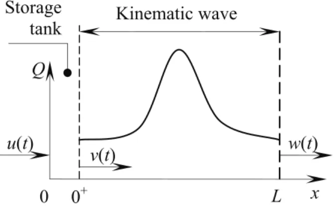
where φ(x) is a vector containing all the parameters on which Q locally depends (e.g. Manning’s friction coefficient, the bed slope of the channel, etc.). The parameter vector φ is constant in time. The flow model (31–33) corresponds to a kinematic wave routing model over the reach (0, L], with the point x = 0 serving as a controlled storage tank (see Fig. 1).
The input discharge to the tank (at x = 0−
) is given by u(t), while the output discharge of the tank v(t) at x = 0+ is given by Eq. (33b). The
discharge wave travels into the channel (x ∈ (0, L]) according to a kinematic wave approximation (Eqs. (32, 33a)). Although the discharge law (33) is discontinuous, the system (32–33) is conservative because it verifies Eq. (28) and no particular assumption needs to be made about the continuous char-acter of A and Q in the calculation of the integrals in Eq. (28). Note that S,
Figure 1: Conceptual representation of the model (32–33).
as defined in Eq. (31), includes not only the volume of water stored within the reach (0, L] but also the volume of water present in the controlled storage tank.
The total volume of water stored in the reach [0, L] is given by S = Z L 0 (A(x, t) + δ(x)S0(t))dx = S0(t) + Z L 0 A(x, t)dx
where δ(x) is Dirac’s distribution and S0(t) is the volume of water stored in
the tank.
The characteristic form of Eqs. (32–33a) is known to be [11] dQ dt = 0 for dx dt = µ (34a) µ = ∂Q ∂A (34b)
where µ is the propagation speed of the wave. Applying Eq. (34a) between x = 0+ and x = L yields
Q(L, t) = Q(0+, t − τ), (35)
where τ is the travel time of the wave between x = 0+ and x = L. Since
there is a one-to-one relationship between Q and A at all points, µ depends only on Q and τ is a function of Q alone. Consequently, τ is a function of w.
Noticing that Q(0, t) = u(t), v(t) = Q(0+, t) and Q(L, t) = w(t), Eqs. (33b) and (35) become dv dt = 1 K(u(t) − v(t)) (36a) w(t) = v(t − τ) (36b)
which is precisely the nonlinear model with delay (22). Since the model (31– 33) is conservative, the nonlinear model with delay (22) is also conservative. We now compare the obtained simplified models to the original PDE models using simulated and real data.
5. Applications of the Nonlinear Models
We first perform simulations with the model derived based on the diffusive wave equation. Then, we test the model based on the Saint-Venant equations on real data.
The nonlinear system being composed of a nonlinear system with a delay in output, the nonlinear system without delay is first solved with a Runge-Kutta method of order 4, and the delayed output is computed in a second step.
5.1. Nonlinear Model Simulations
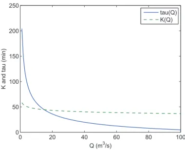
We consider a river of length L = 10 km, width W = 8 m, Manning coefficient n = 0.05, slope Sb = 0.0004. The parameters K and τ of the
nonlinear model can be computed as functions of the discharge Q using eqs. (14–15) and (2–3). The results are depicted in Fig. 2. We see that the time delay τ varies between 204 min and 5 min when the discharge varies between 1 m3/s and 100 m3/s, while the time constant K varies between 58 min and
36 min.
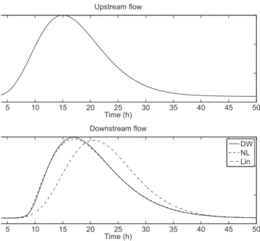
These model parameters are used to compute the output of the simpli-fied model given by Eq. (22). Validation is done by comparing the output of the proposed nonlinear model with that of the diffusive wave model (1) for the same input data. The diffusive wave equation (1) is solved using a semi-implicit finite difference scheme (Crank-Nicholson scheme). We also compare the output of the proposed model (22) with that given by the linear Hayami model obtained by linearization around the initial discharge u(0). The simulation results are depicted in Fig. 3.
0 20 40 60 80 100 0 50 100 150 200 250 Q (m3/s)
K and tau (min)
tau(Q) K(Q)
Figure 2: Values of parameters K and τ as functions of Q
The nonlinear model with delay reproduces well the behavior of the river, and is very close to the diffusive wave model. One notices that the main characteristic of these rivers for low flows, i.e. the variation of the delay with the discharge, is taken well into account by the nonlinear model with delay, whereas this is not the case for the linear model.
5.2. Comparison with Real Data
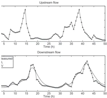
We now test the simplified model (26) based on the linearized Saint-Venant equations. To this end, we use the set of real data used by Baptista and Michel to evaluate the performance of the quadratic lag and route model [3]. This data consists of propagation of dam releases on the Jacui river in Brazil between Itauba and Volta Grande, recorded at a time step of 30 minutes [2].
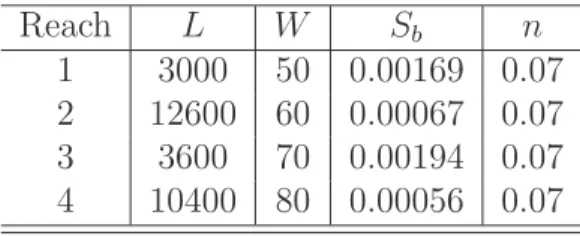
The geometry of the river reaches is detailed in Table 1. The downstream flow is computed by using a cascade of nonlinear models, one for each reach. The input of the first reach is the upstream flow, and the computed down-stream flow is used as an input for the next reach. The computation is done for the five reaches in series, and only the downstream flow of the last reach is depicted in the graphical results.
5 10 15 20 25 30 35 40 45 50 Time (h) Upstream flow 5 10 15 20 25 30 35 40 45 50 Time (h) Downstream flow DW NL Lin
Figure 3: Comparison between the diffusive wave model (DW —), the nonlinear model of first order with delay (NL – –) and the linear Hayami model obtained for Q0= Q(0) (Lin
–·–)
Simulation results are depicted in Fig. 4. The model only uses the data given in Table 1 and the upstream flow to compute the downstream flow. The Nash-Sutcliffe coefficient is equal to 0.91, which is rather good. We also depict on the same graph the simulation results obtained with a full nonlinear Saint-Venant model, which also uses the geometry of the five reaches in series to compute the downstream flow. A uniform depth boundary condition is used at the downstream end.
The simplified nonlinear model leads to almost identical results as those obtained with the Saint-Venant equations, which explains why the two curves are indistinguishable. This shows that a simplified nonlinear model can effi-ciently reproduce the flow transfer described by the full Saint-Venant equa-tions in this case.
Table 1: Physical characteristics of the Jacui river reaches Reach L W Sb n 1 3000 50 0.00169 0.07 2 12600 60 0.00067 0.07 3 3600 70 0.00194 0.07 4 10400 80 0.00056 0.07 5.3. Model Calibration
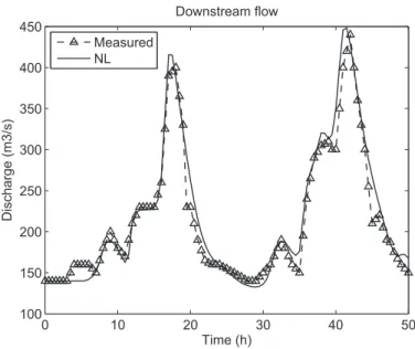
From the simulation results in Fig. 4, it seems that the model leads to a larger attenuation than in reality, i.e. the time constant K is too large. This could come from a bad calibration of the Manning coefficient, or a bad estimation of the geometry of the river reaches. To illustrate a possible application of the model, we now consider the river as a single reach, and try to identify physical parameters based on the input-output behavior of the system. To this end, we fix the length of the river reach L = 29600 m and the Manning coefficient n = 0.07, and we identify an average geometry (width B and slope Sb) by minimizing the sum of the quadratic error between the
measured and the computed downstream flows.
The optimization resulted in an average width B = 55.6 m and an average slope Sb = 0.00089. The Nash coefficient is then equal to 0.95 instead of 0.91
for the simulation case without calibration (see the simulation results in Fig. 5). This example illustrates a possible use of the model for parameter estimation. However, the analysis of the calibration of a model in the case of partially known or simplified geometry is out of the scope of this paper. This subject would require a more in depth study. This simple example is just here to show a possible application of the proposed simplified model. 6. Conclusion
We described in this paper a way to obtain a simple DDE nonlinear model from a quasilinear PDE. After linearization around a reference regime, the cumulant matching method is applied to the linear PDE in order to get an approximation of its irrational transfer function. Then a single nonlinear model is obtained from the family of linear ones indexed by the value of the discharge around which they were linearized. This methodology was applied on two different nonlinear PDEs: the diffusive wave equation and the
Saint-5 10 15 20 25 30 35 40 45 50 Time (h) Upstream flow 5 10 15 20 25 30 35 40 45 50 Time (h) Downstream flow Measured NL SV
Figure 4: Simulation on real data from the Jacui river. Measured upstream flow (−△−), measured downstream flow (−△−), downstream flow simulated by the nonlinear model (—) and by the Saint-Venant equations (– –)
Venant equations. A first order nonlinear model with delay is obtained as an approximation of the nonlinear PDE.
The simplified nonlinear model has the advantage to be directly related to physical parameters, as the length of the river stretch L, the slope Sb,
Manning coefficient n and the width W . This model can be used for many different purposes:
• For quick simulation purposes, as it is easier to implement than a com-plete numerical resolution of the initial partial differential equation, • For identification purposes: a model-based identification usually
re-quires numerous simulations of the model, which is time-consuming. A simpler model can be simulated more quickly,
• For controller design, as some dams located upstream can be used to control the discharge downstream of the river (see e.g. [19, 21, 6]).
0 10 20 30 40 50 100 150 200 250 300 350 400 450 Time (h) Discharge (m3/s) Downstream flow Measured NL
Figure 5: Calibration of the simplified nonlinear model on real data from the Jacui river. Measured downstream flow (−△−) and downstream flow simulated by the nonlinear model (—).
Finally, the proposed approach can be generalized to various other cases, such as the model of first order with delay derived by [25] for rivers or canals with a backwater curve. The proposed method provides a rigorous way to derive a nonlinear model from a set of linear models, which can prove very useful in the hydrological context.
Acknowledgements
The help of Julien Lerat, Charles Perrin and Marci´o Baptista who pro-vided the data of the Jacui river is gratefully acknowledged.
A. Derivation of the Hayami Transfer Function
The linear partial differential equation (4) has an analytical solution for simple inputs (steps or ramps) (see e.g. [24]). Using Laplace transform, one can express the input-output relations as a transfer function [1]. Given a function f (x, t), t ≥ 0, its temporal Laplace transform, denoted L(f(x, t)),
or ˆf (x, s) is given by: L(f(x, t)) = ˆf (x, s) = Z ∞ 0 e−stf (x, t)dt. We then have: Lµ ∂f (x, t) ∂t ¶ = s ˆf (x, s) − f(x, 0), and Lµ ∂f (x, t) ∂x ¶ = ∂ ˆf (x, s) ∂x , and Lµ ∂ 2f (x, t) ∂x2 ¶ = ∂ 2f (x, s)ˆ ∂x2 .
Applying Laplace transform to the system (4) leads to: E0
∂2q(x, s)ˆ
∂x2 − Θ0
∂ ˆq(x, s)
∂x − sˆq(x, s) = q(x, 0).
This is in fact an ordinary differential equation in the variable x, whose characteristic equation
E0λ2− Θ0λ − s = 0
has two solutions if E0 6= 0.
With the hypothesis q(x, 0) = 0, the solution ˆq(x, s) is of the following form: ˆ q(x, s) = A1(s)eλ1(s)x+ A2(s)eλ2(s)x, with λ1(s) = Θ0−pΘ20+ 4E0s 2E0 , λ2(s) = Θ0+pΘ20+ 4E0s 2E0 .
The boundary conditions can now be used to specify variables A1(s)
and A2(s). The downstream boundary condition leads to A2(s) = 0, since
ℜ(λ2(s)) > 0 for ℜ(s) > 0. The upstream boundary condition leads to
A1(s) = ˆq(0, s). Finally, the Hayami transfer function is obtained as follows:
ˆ q(x, s) = FHayami(x, s)ˆq(0, s) with FHayami(x, s) = e Θ0−√Θ20+4E0s 2E0 x.
B. Derivation of the Saint-Venant Transfer Function
Following the approach developed by [17, 16], the Saint-Venant trans-fer function can be computed based on the linearized equations. Applying Laplace transform to Eqs. (24), and assuming zero initial conditions leads to: ∂ ∂x µ ˆq ˆ y ¶ = Asµ ˆq ˆ y ¶ with As= Ã 0 −W0s 2gSb−V0s W0V0C02(1−F02) 2V0s+g(1+κ)Sb C2 0(1−F02) ! . Matrix As has two eigenvalues, given by:
λ(s) = as + b ±√cs2+ ds + b2,
with a, b, c and d given by Eqs. (25).
Assuming a semi-infinite channel leads to: ˆ q(x, s) = eλSV(s)xq(0, s)ˆ with λSV(s) = as + b − √ cs2+ ds + b2. References
[1] A. Angot. Compl´ements de math´ematiques `a l’usage des ing´enieurs de l’´electrotechnique et des t´el´ecommunications. Masson et Cie, Paris, 6th edition, 1972. in French.
[2] M. Baptista. Contribution `a l’´etude de la propagation de crues en hy-drologie. PhD thesis, Ecole Nationale des Ponts et Chauss´ees, Paris, Septembre 1990.
[3] M. Baptista and C. Michel. Influence des caract´eristiques hydrauliques des biefs sur la propagation des pointes de crue. La Houille Blanche, 2:141–148, 1990.
[4] J.-P. Baume, J. Sau, and P.-O. Malaterre. Modeling of irrigation channel dynamics for controller design. In Conf. on Systems, Man and Cyber-netics, SMC’98, pages 3856–3861, San Diego, 1998.
[5] P.L.F. Bentura and C. Michel. Flood routing in a wide channel with a quadratic lag-and-route method. Hydrological Sciences, 42(2):169–189, 1997.
[6] G. Besan¸con, D. Georges, and Z. Benayache. Towards nonlinear delay-based control for convection-like distributed systems: the example of water flow control in open channel systems. Networks Heterogeneous Media, 4(2):211–222, 2009.
[7] K.J. Beven. Prophecy, reality and uncertainty in distributed hydrologi-cal modelling. Adv. Water Resourc., 16:41–51, 1993.
[8] L.A. Camacho and M.J. Lees. Multilinear discrete lag-cascade model for channel routing. J. of Hydrology, 226:30–47, 1999.
[9] V.T. Chow. Open-channel hydraulics. McGraw-Hill, New York, 1988. 680 p.
[10] J.A. Cunge. On the subject of a flood propagation computation method (Muskingum method). J. Hydr. Res., 7(2):205–230, 1969.
[11] J.A. Cunge, F.M. Holly, and A. Verwey. Practical aspects of computa-tional river hydraulics. Pitman Advanced Publishing Program, 1980. [12] J.C.I. Dooge, J.J. Napi´orkowski, and W.G. Strupczewski. The linear
downstream response of a generalized uniform channel. Acta Geophys. Polon., XXXV(3):279–293, 1987.
[13] S. Hayami. On the propagation of flood waves. report, Disaster Preven-tion Institute, University of Kyoto, 1951.
[14] M. Lal and R. Mitra. A comparison of transfer function simplification methods. IEEE Trans. Autom. Contr., 19(5):617–618, 1974.
[15] X. Litrico. Nonlinear diffusive wave modeling and identification for open-channels. J. Hydraul. Eng., 127(4):313–320, 2001.
[16] X. Litrico and V. Fromion. Frequency modeling of open channel flow. J. Hydraul. Eng., 130(8):806–815, 2004.
[17] X. Litrico and V. Fromion. Modeling and control of hydrosystems. Springer, London, 2009.
[18] X. Litrico and D. Georges. Robust continuous-time and discrete-time flow control of a dam-river system (I): Modelling. Appl. Math. Mod., 23(11):809–827, 1999.
[19] X. Litrico and D. Georges. Robust continuous-time and discrete-time flow control of a dam-river system (II): Controller design. Appl. Math. Mod., 23(11):829–846, 1999.
[20] X. Litrico and V. Guinot. Discussion of “Development and Verifi-cation of an Analytical Solution for Forecasting Nonlinear Kinematic Flood Waves” by Sergio E. Serrano, Journal of Hydrologic Engineer-ing, July/August 2006, Vol. 11, No. 4, pp. 347-353. J. of Hydrologic Engineering, 12(6):703–705, 2007.
[21] X. Litrico and J.-B. Pomet. Nonlinear modeling and control of a long river stretch. In European Control Conference, Cambridge, UK, 2003. [22] P.-O. Malaterre. Mod´elisation, analyse et commande optimale LQR d’un
canal d’irrigation. PhD thesis, ENGREF–Cemagref, 1994. (in French). [23] W.A. Miller and J.A. Cunge. Simplified equations of unsteady flow, pages 183–257. Water Resources Publications, Fort Collins, CO, 1975. [24] R. Moussa and C. Bocquillon. Criteria for the choice of flood routing
methods in natural channels. J. of Hydrology, 186(1-4):1–30, 1996. [25] S. Munier, X. Litrico, G. Belaud, and P.-O. Malaterre. Distributed
approximation of open-channel flow routing accounting for backwater effects. Adv. Water Resourc., 31:1590–1602, 2008.
[26] M. Perumal, T. Moramarco, and F. Melone. A caution about the mul-tilinear discrete lag-cascade model for flood routing. J. of Hydrology, 338(3-4):308–314, May 2007.
[27] V.M. Ponce and F.D. Theurer. Accuracy criteria in diffusion routing. J. of Hydraulics Division, 108(HY6):747–757, 1982.