Aggregation and multi-level control in discrete event dynamic systems

August 1989 LIDS-P-1902

AGGREGATION AND MULTI-LEVEL CONTROL IN

DISCRETE EVENT DYNAMIC SYSTEMS

1

Cirneyt M. Ozveren2 Alan S. Willsky2

August 7, 1989

Abstract

In this paper we consider the problem of higher-level aggregate modelling and con-trol of discrete-event dynamic systems (DEDS) modelled as finite state automata in which some events are controllable, some are observed, and some represent events to be tracked. The higher-level models considered correspond to associating specified sequences of events in the original system to single macroscopic events in the higher-level model. We also consider the problem of designing a compensator that can be used to restrict microscopic behavior so that the system will only produce strings of these primitive sequences or tasks. With this lower level control in place we can con-struct higher-level models which typically have many fewer states and events than the original system. Also, motivated by applications such as flexible manufactur-ing, we address the problem of constructing and controlling higher-level models of interconnections of DEDS. This allows us to "slow down" the combinatorial explosion typically present in computations involving interacting automata.

'Research supported by the Air Force Office of Scientific Research under Grant AFOSR-88-0032 and by the Army Research Office under Grant DAAL03-86-K0171.

1 Introduction

The study of complex systems has frequently prompted research on tools for aggre-gation and multi-level analysis. In this paper, we study such tools in the context of Discrete Event Dynamic Systems (DEDS). DEDS have been studied extensively by computer scientists, and recently, the notion of control of a DEDS has been intro-duced by Wonham, Ramadge, et al. [1,7,8,9]. This work assumes a finite state model in which certain events in the system can be enabled or disabled. The control of the system is achieved by choice of control inputs that enable or disable these events. We also consider a similar model in our work.

A major issue of concern in the work of Wonham and Ramadge, as well as other work on DEDS is that of computational complexity, and the goal of this paper is to address certain issues of complexity. In particular, in many applications the desired range of behavior of a DEDS is significantly smaller and more structured than its full range of possible behaviors. For example, a workstation in a flexible manufacturing system may have considerable flexibility in the sequence of operations it performs. However, only particular sequences correspond to useful tasks. This idea underlies the notion of a legal language introduced in [8]. In the analysis described in this paper we use it as well to develop a method for higher-level modelling and control in which a sequence of events corresponding to a task is mapped to a single macro-event at the higher-level. Also, in DEDS described as interconnections of subsystems the overall state space for the entire system can be enormous. However, in many applications, such as a flexible manufacturing system consisiting of interconnections of workstations, the desired coordination of the subsystems is at the task level, and thus we can consider the interactions of their individual aggregate models. These

1 INTRODUCTION 2

higher-level characterizations allow us to represent sets of states by a single state and sets of strings by a single event. We thus achieve both spatial and temporal aggregation that can greatly reduce the apparent computational explosion arising in the analysis of extremely complex systems.

The work described in this paper builds on several of our previous papers [2,3,4, 5,6] and can be viewed as the culmination of an effort to develop a regulator theory for DEDS. As we will see, our development will involve controlling the system so that its behavior is restricted to completing the desired tasks. To address this, we will rely on the notions of tracking and restrictability that we developed in [5]. The latter of these is closely related to the notion of constraining behavior to a legal language. However, by describing the desired behavior in terms of primitive tasks, we achieve significant efficiencies, and through the use of the notion of eventual restrictability we are able to directly accomodate the phenomenon of set-up, i.e., the externally irrelevant transient behavior arising when one switches between tasks.

We will see that many of the components of our work are relevant here. In particular, our notion of stability [6], i.e., of driving the system to a specified set of states is central to most of our constructions. Furthermore, since we assume a model in which only some events are observed, we will need to make use of our results in observability [3] and output stabilization [4]. Finally, in order to derive an upper-level model, it will be necessary to be able to use our observations to reconstruct the sequence of tasks that has been performed. This is closely related to the problem of invertibility stated in [2].

In the next section, we introduce the mathematical framework considered in this paper and summarize those parts of our previous work that will be used in the sequel.

In Section 3, we formulate a notion of modelling based on a given set of macro-events or primitives, which allows us to characterize higher-level models of DEDS. In Sec-tion 4, motivated by flexible manufacturing systems, we define tasks as primitives, introduce notions of reachability and observability of tasks, and construct task com-pensators and detectors. Using these components, we construct an overall task-level control system which accepts task requests as input and controls the system to achieve the desired sequence. This leads to a simple higher-level model whose transitions only involve the set-up and completion of tasks. In Section 5, we show how a system com-posed of m subsystems can be modelled by a composition of the higher-level models of each subsystem. Also, we illustrate our approach using a simple manufacturing example, and show how the overall control of the task sequence of this system can be achieved by a higher-level control acting on the composite task-level model. Finally, in Section 6, we summarize our results and discuss several directions for further work.

2 BACKGROUND AND PRELIMINARIES 4

2 Background and Preliminaries

2.1 System Model

The class of systems we consider are nondeterministic finite-state automata with intermittent event observations. The basic object of interest is the quintuple:

G = (X, E, O, r, E) (2.1)

where X is the finite set of states, with n = IX 1, E is the finite set of possible events, (4 C E is the set of controllable events, r C E is the set of observable events, and :-C C is the set of tracking events. Also, let U = 2E denote the set of admissible control inputs consisting of a specified collection of subsets of E. The dynamics defined on G are as follows, where 4 denotes the complement of D:

x[k + 1] E f(x[k],[k + 1]) (2.2)

a[k + 1] E (d(x[k]) n u[k]) U (d(x[k]) nT ) (2.3)

Here, x[k] E X is the state after the kth event, oi[k] E E is the (k + 1)st event, and u[k] E U is the control input after the kth event. The function d : X -- 2' is a set-valued function that specifies the set of possible events defined at each state (so that, in general, not all events are possible from each state), and the function

f : X x E -- X is also set-valued, so that the state following a particular event

is not necessarily known with certainty. We assume that (~ C r. This assumption simplifies the presentation of our results, but it is possible to get similar results, at a cost of additional computational complexity, if it is relaxed.

Our model of the output process is quite simple: whenever an event in r occurs, we observe it; otherwise, we see nothing. Specifically, we define the output function

h

E

-- r U {e}, where e is the "null transition", by

or ifuer

h(r) = (2.4)

e otherwise

Then, our output equation is

-y[k + 1] = h(oa[k + 1]) (2.5)

Note that h can be thought of as a map from E* to

r*,

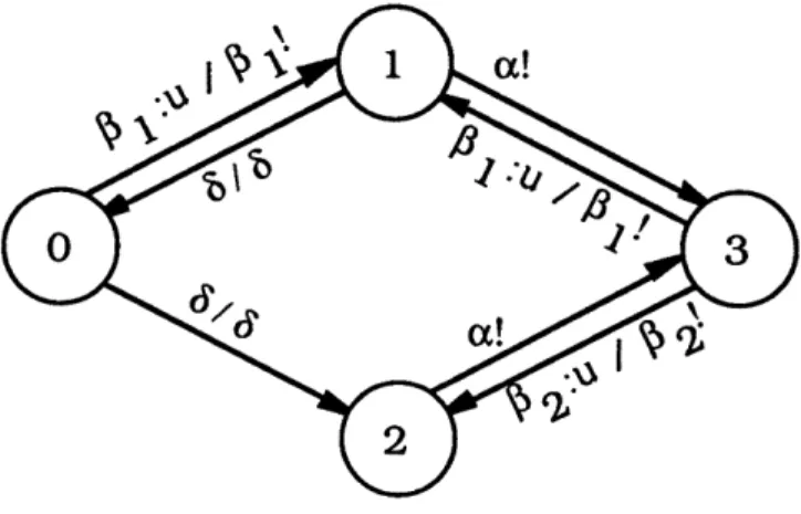
where r* denotes the set of all strings of finite length with elements in r, including the empty string e. In particular, h(al ... Oa,) = h(l,) . h(oa,).

The set E, which we term the tracking alphabet, represents events of interest for tracking purposes. This formulation allows us to define tracking over a selected alphabet so that we do not worry about listing intermediary events that are not important in tracking. We use t : E* --+*, to denote the projection of strings over E into A*. The quintuple A = (G, f, d, h, t)3 representing our system can also be visualized graphically as in Figure 2.1. Here, circles denote states, and events are represented by arcs. The first symbol in each arc label denotes the event, while the symbol following "/' denotes the corresponding output. Finally, we mark the

controllable events by ":u" and tracking events by "!". Thus, in this example, X =

{0,1,2,3}, E = {(, I1, ]2, 6}, = { 3(1, 2 }),

r

= {6(,

1,

P

2

},

and = {a,/ 1,, 2} .

There are several basic notions that we will need in our investigation. The first is the notion of liveness. Intuitively, a state is alive if it cannot reach any state at which no event is possible. That is, x E X is alive if Vy E R(A, x), d(y) $& 0. Also, we say that Q c X is alive if all x E Q, are alive, and we say that A is alive if X is alive.

3_{0n occasion, we will construct auxiliary automata for which we will not be concerned with either}

2 BACKGROUND AND PRELIMINARIES 6

Figure 2.1: A Simple Example

We will assume that this is the case. A second notion that we need is the composition of two automata, Ai = (Gi, fi, di, hi) which share some common events. Specifically, let S = El n f2 and, for simplicity, assume that rl n S = r2 n S (i.e., any shared

event observable in one system is also observable in the other), 1l nS = -2 n S, and E1 n S = E2n S. The dynamics of the composition are specified by allowing

each automaton to operate as it would in isolation except that when a shared event occurs, it must occur in both systems. Mathematically, we denote the composition by

A12 = Al |1 A2 = (G12, f1 2, d12, hl2, t12), where G12 = (X1 X X2, 1 U '2, (1 U (2 , lF1 U r2, 1 U ,2 ) (2.6) fi2(x,o) = fi(xl, ) x f2(x2, a) (2.7) d1 2(x) = (dl(xl) n) u (d2(x2) n ) U (dl(xl) n d2(x2)) (2.8) hl(a) ifaEFrl hl2(f) = h2(ff) ifa E 2 (2.9) l e otherwise

tl(ao) if O E -1

t12(f) = t2(o) if a E 2 (2.10)

e otherwise

Here we have extended each fi to all of E1UJE2 in the trivial way, namely, fi(xi, a)-:i

if a ~ Ei. Note also that h12 and t12 are well-defined.

2.2 Languages

Let L be a regular language over an alphabet E (see [8]). As in [8], let (AL, XO) be a minimal recognizer for L. Given a string s E L, if s = pqr for some p, q and r over E then we say that p is a prefix of s and r is a suffix of s. We also use s/pq to denote the suffix r. Also, we say that q is a substring of s. Finally, we need the following characterization of the notion of liveness in the context of languages:

Definition 2.1 Given L, s E L has an infinite extension in L if for all integers i > Is l,

there exists r E L, Irl = i such that s is a prefix of r. L is prefix closed if all the prefixes of any s E L are also in L. L is a complete language if each string in L

has an infinite extension in L and L is prefix closed. L

For any language L, we let Lc denote the prefix closure of L, i.e.

L'

=

{p E E*Ip is a prefix of some s E L} (2.11)

2.3 Forced Events

In our development we will find it necessary to construct automata in which certain events can be forced to occur regardless of the other events defined at the current state and in fact can only occur if they are forced. The following shows that we can

2 BACKGROUND AND PRELIMINARIES 8

capture forced events in our present context with a simple construction. Given x E X let d l(x) denote the set of forced events defined at x and let d2(x) denote the other -events (controllable or uncontrollable) defined at x. We introduce a new controllable event # and a new state x' as follows: We redefine d(x) as d1(x) U pt so that all events defined at x are now controllable and we define f(x, p) = {x'}. Also, we define

d(x') = d2(x) so that f(x', a) = f(x, o) for all a E d2(x). If in addition, we impose the restriction that only one event can be enabled at a time at state x, then we can treat forced events as controllable events in our framework. Thus, if we decide to

force an event at x, then we enable only that event, and if we decide not to force any events, then we enable p.

2.4 Stability and Stabilizability

In [6], we define a notion of stability which requires that trajectories go through a given set E infinitely often:

Definition 2.2 Let E be a specified subset of X. A state x E X is E-pre-stable if there exists some integer i such that every trajectory starting from x passes through

E in at most i transitions. The state x e X is E-stable if A is alive and every state reachable from x is E-pre-stable. The DEDS is E-stable if every x E X is E-stable

(Note that E-stability for all of A is identical to E-pre-stability for all of A).

By a cycle, we mean a finite sequence of states x1, x2,... xk, with Xk = x1, so that there exists an event sequence s that permits the system to follow this sequence of states. In [6] we show that E-stability is equivalent to the absence of cycles that do not pass through E. We refer the reader to [6] for a more complete discussion of this subject and for an O(n2) test for E-stability of a DEDS. Finally, we note that in [6]

and Definition 2.2 we require livenes in order for a system to be stable. However, on occasion, in this paper (see, for example, the following section on the tracking alphabet), it is useful to allow trajectories to die provided that they die in E. It is straightforward to check that all of our results in [6] also hold for this slightly more general notion of stability.

In [6], we also study stabilization by state feedback. Here, a state feedback law is a map K : X -+ U and the resulting closed-loop system is AK = (G, f, dK, h, t) where

dK(x) = (d(x) n K(x)) U (d(x) n T) (2.12)

Definition 2.3 A state x E X is E-pre-stabilizable (respectively, E-stabilizable) if there exists a state feedback K such that x is E-pre-stable (respectively, E-stable) in AK. The DEDS is E-stablilizable if every x E X is E-stabilizable. O

If A is E-stabilizable, then (as we show in [6]), there exists a state feedback K such that AK is E-stable. We refer the reader to [6] for a more complete discussion of this subject and for an O(n3) test for E-stabilizability of a DEDS, which also provides a

construction for a stabilizing feedback.

2.5 Tracking Alphabet

The tracking alphabet provides the flexibility to specify strings that we desire to track over an alphabet which may be much smaller than the entire event alphabet E. Note that if there exists a cycle in A that consists solely of events that are not in E, then the system may stay in this cycle indefinitely, generating no event in E. To avoid this possibility, we assume that it is not possible for our DEDS to generate arbitrarily long sequences of events in E. A necessary and sufficient condition for

2 BACKGROUND AND PRELIMINARIES 10

checking this is that if we remove the events in -, the resulting automaton AlE must be Dt-stable, where

Dt = {x E Xld(x) C -} (2.13)

This is not difficult to check and will be assumed.

2.6 Invariance

In [6], we define the following notion of dynamic invariace in order to characterize stability in terms of pre-stability:

Definition 2.4 A subset Q of X is f-invariant if f(Q, d) c Q where

f(Q, d) =

U

f(, d(x)) xEQ

In [6] we show that the maximal stable set is the maximal f-invariant set in the maximal pre-stable set.

In the context of control, the following notion, also presented in [6], is a well-known extension of f-invariance:

Definition 2.5 A subset Q of X is (f, u)-invariant if there exists a state feedback K

such that Q is f-invariant in AK. °

However, recall that in general we also need to preserve liveness. Thus we have the following:

Definition 2.6 A subset Q of X is a sustainably (f, u)-invariant set if there exists a state feedback K such that Q is alive and f-invariant in AK.

Given any set V C X, there is a maximal sustainably (f,u)-invariant subset W of V with a corresponding unique minimally restrictive feedback K. That is K disables

as few events as possible in order to keep the state within W.

2.7 Observability and Observers

In [3], we term a system observable if the current state is known perfectly at in-termittent but not necessarily fixed intervals of time. Obviously, a necessary condi-tion for observability is that it is not possible for our DEDS to generate arbitrarily long sequences of unobservable events, i.e., events in F, the complement of F. A necessary and sufficient condition for checking this is that if we remove the observ-able events, the resulting automaton Air = (G, f, d n r, h, t) must be Do-stable,

where Do is the set of states that only have observable transitions defined, i.e.,

Do = {x E X d(x) n = 0}. This is not difficult to check and will be assumed. Let us now introduce some notation that we will find useful:

* Let x --+ y denote the statement that state y is reached from x via the occurence of event sequence s. Also, let x -+* y denote that x reaches y in any number of transitions, including none. For any set Q C X we define the reach of Q in A as:

R(A, Q) = {y E X13x E Q such that x -A* y} (2.14)

* Let

Yo = {x E XXI y E X,a E E, such that x E f(y,'y)} (2.15)

Yj = {x X3y E X,Y E r, such that xE f(y,-y)} (2.16)

2 BACKGROUND AND PRELIMINARIES 12

Thus, Y is the set of states x such that either there exists an observable tran-sition defined from some state y to x (as captured in Y1) or x has no transitions

defined to it (as captured in Yo). Let q = IYI.

* Let L(A, x) denote the language generated by A, from the state x E X, i.e.,

L(A, x) is the set of all possible event trajectories of finite length that can be

gen-erated if the system is started from the state x. Also, let L(A) = UxEX L(A, x) be the set of all event trajectories that can be generated by A.

In [3], we present a straightforward design of an observer that produces "esti-mates" of the state of the system after each observation y[k] E F. Each such estimate is a subset of Y corresponding to the set of possible states into which A transi-tioned when the last observable event occurred. Mathematically, if we let a function

x: h(L(A)) -+ 2' denote the estimate of the current state given the observed output

string t E h(L(A)), then

i(t) = {x E Y13y E X and s E Lf(A,y) such that h(s) = t and x E f(y,s)} (2.18)

The observeris a DEDS which realizes this function. Its state space is a subset Z of 2Y, and its full set of events and set of observable events are both F. Suppose that the present observer estimate is x[k] E Z and that the next observed event is

y[k + 1]. The observer must then account for the possible occurence of one or more

unobservable events prior to y[k + 1] and then the occurrence of O[k + 1]:

5[k + 1] = w(5[k],'y[k -+ 1]) - UXER(AIr,£[k]) f(x,Y[k + 1]) (2.19)

Ay[k + 1] E v(&[k])

-

h(UWER(AIr,i[k]) d(x)) (2.20)

The set Z is then in the reach of {Y} using these dynamics, i.e., we start the observer in the state corresponding to a complete lack of state knowledge and let it evolve.

Our observer then is the DEDS O = (F, w, v, i), where F = (Z, F, r, ,) and i is the identity output function. In some cases, we will treat the observer as a controlled

system and discuss stabilizing it. Then, Equation 2.20 becomes

y[k + 1] E v(5[k]) - h(UxER(Alr,i[k])(d(x) n u[k]) U (d(x) n

¥))

(2.21) In [3], we show that a system A is observable iff O is stable with respect to its singleton states. We also show that if A is observable then all trajectories from an observer state pass through a singleton state in at most q2transitions.

In [3] we also define a notion of recurrency. In particular, we say that a state x is a recurrent state if it can be reached by an arbitrarily long string of events. We let Zr denote the set of recurrent states of the observer O.

2.8

Compensators

In [5], we define a compensator as a map C : X x E* -- U which specifies the set of controllable events that are enabled given the current state and the entire event trajectory up to present time. Given a compensator C, the closed loop system Ac is the same as A but with

a[k + 1] E dc(x[k], s[k]) = (d(x[k]) n C(x[k], s[k])) U (d(x) n a) (2.22)

where s[k] = a[0] ... a[k] with a[0] = e. Here we have somewhat modified notation in that we allow dc to depend both on x[k] and s[k]. It is not difficult to show that we can always write Ac as an automaton (with corresponding "d" depending only on the state), which will take values in an expanded state space, representing the cross-product of the state spaces of A and C. For an arbitrary choice of C, its state space (i.e., an automaton realizing the desired map) may be infinite. As show in [5]

2 BACKGROUND AND PRELIMINARIES 14

for our purposes we can restrict attention to compensators which can be realized by finite state machines.

In [4] we define an output compensator as a map C : r* -- U. Then, the closed loop system Ac is the same as A but with:

o[k + 1] E dc(x[k], s[k]) (d(x[k]) n C(h(s[k]))) U (d(x) n A) (2.23)

One constraint we wish to place on our compensators is that they preserve liveness. Thus, suppose that we have observed the output string s, so that our observer is in x(s) and our control input is C(s). Then, we must make sure that any x reachable from any element of k(s) by unobservable events only is alive under the control input

C(s). That is, for all x E R(Alr, x(s)), dc(x, s) should not be empty. This leads to

the following:

Definition 2.7 Given Q c X, F c I, F is Q-compatible if for all x E R(Alr, Q),

(d(x) n F) U (d(x) nl

A)

/

0.

An observer feedback K : Z -+ U is A-compatible if for all x E Z K(.) is

i-compatible.

A compensator C:

r*

U is A-compatible if

for all s E h(L(A)), C(s) is

i(s)-compatible.

O

2.9 Stabilization by Output Feedback

In [4] we define a notion of stabilization by output feedback which requires that we can force the trajectories to go through E infinitely often using an output compensator:

Definition 2.8 A is output stabilizable (respectively, output pre-sta-bilizable) with respect to E if there exists an output compensator C such that Ac is E-stable (respectively, E-pre-stable). We term such a compensator an output stabilizing (respectively, output pre-stabilizing) compensator. L

Note that this definition implicitly assumes that there exists an integer n8 such that the trajectories in Ac go through E in at most n, observable transitions. In [4] we show that n, is at most q3, and, using this bound, we show that output pre-stabilizability and liveness are necessary and sufficient for output pre-stabilizability, as is the case for stabilizability and pre-stabilizability.

2.10 Eventual Restrictability

In [5] we define a notion of restrictability which requires that we can force the system to generate strings in a desired language defined over -:

Definition 2.9 Given x E X and a complete language L over E, x is L-restrictable if there exists a compensator C: X x E* -- U such that the closed loop system

Ac is alive and t(L(Ac,x)) C L. Given Q c X, Q is L-restrictable if all x E Q are L-restrictable. Finally, A is L-restrictable if X is L-restrictable. O

We also define a notion of eventual restrictability which requires that we can restrict the system behavior in a finite number of transitions. In the following, (E U {e})n" a denotes the set of strings overE that have length at most n,:

Definition 2.10 Given x E X and a complete language L over

E,

x is eventually

L-restrictable if there exists an integer n, and a compensator C: X x E* -- U such that the closed loop system Ac

is

alive and t(L(Ac, x)) c (E U {e})naL. Given Q c X, Q is eventually L-restrictable if all x E Q are eventually L-restrictable. Finally, A is eventually L-restrictable if X is eventually L-restrictable. I)

We refer the reader to [5] for a more complete discussion of this subject. We now turn our attention to eventual restrictability using an output compensator. The following,

2 BACKGROUND AND PRELIMINARIES 16

although not included in [5], is a straightforward use of tools that we have developed in [4] and [5]:

Definition 2.11 Given a complete language L over E we say that A is eventually L-restrictable by output feedback if there exists an integer no and an output com-pensator C :

r*

-- U such that Ac is alive and for all x E X, t(L(Ac,x)) C

(E U {e})noL. Such a C is called an L-restrictability compensator.

iJ

We construct a test for eventual restrictability by output feedback as follows: Given

L, let (AL, xoL ) be a minimal recognizer for L and let ZL denote its state space. Let A'L be an automaton which is the same as AL except that its state space is ZIL = ZL U {b}

where b is a state used to signify that the event trajectory is no longer in L. This is the state we wish to avoid. Also, we let d'(x) = a for all x E ZL, and

f(x, a) =

J

fL(x, a) if x i

b

and u E

dL(x)

(2.24)

{b} otherwise

Let 0 denote the observer for A, let A(L) = A II A', and let O(L) = (G(L), wL, vL)

denote the observer for A(L); however, in this case, since we know that we will start

A'L in xo, we take the state space of O(L) as

Z(L) = R(O(L), {{XoL} x X1X E Z}) (2.25)

Let

VO = {z E Z(L)I for all (XL, XA) e Z, XL f b} (2.26) Let E(L) be the largest subset of Vo which is sustainably (f,u)-invariant in O(L) and for which the associated unique minimally restrictive feedback KEL has the property that for any z E Z(L), KEL(:) is k(z)-compatible where

The construction of E(L) and KEL is a slight variation of the algorithm in [6] for the construction of maximal sustainably (f,u)-invariant subsets. Specifically, we begin with any state i E Vo . If there are any uncontrollable events taking z outside V0,

we delete i and work with V1 = Vo \

{:}.

If not, we disable only those controllable events which take z outside V0. If the remaining set of events defined at i is not 5(z)-compatible, we delete z and work with V1 = Vo \ {z}. If not, we tentatively

keep z and choose another element of V,. In this way, we continue to cycle through the remaining elements of V,. The algorithm converges in a finite number of steps (at most IVo121) to yield E(L) and KEL defined on E(L). For z E E(L), we take

KEL(p) =- so that no events are disabled. Consider next the following subset of E(L):

Eo(L) =

{(

E ZlXL x ~ E E(L)} (2.28)

Then,

Proposition 2.12 Given a complete language L over E, A is eventually L-restrictable by output feedback iff there exists an A-compatible state feedback K: Z -+ U

such that the closed loop system OK is Eo(L)-pre-stable.

Proof: (-+) Straightforward by assuming the contrary.

(-) Let us prove this by constructing the desired compensator C : r* -+ U: Given an observation sequence s, we trace it in O starting from the initial state {Y}. Let

be the current state of O given s. There are two possibilities:

1. Suppose that the trajectory has not yet entered Eo(L). Then we use O and the Eo(L)-pre-stabilizing feedback K to compute C(s). In particular,

2 BACKGROUND AND PRELIMINARIES 18

2. When the trajectory in O enters Eo(L), we switch to using the expanded ob-server O(L) and KE(L). In particular, let x' be the state the trajectory in O enters when it enters Eo(L) for the first time, and let s' be that prefix ofs which takes {Y} to x' in 0. Then, we start OL at the state xoL x x' E E(L), and let it evolve. Suppose that sis' takes X4L x x' to i in O(L), then

C(s) = (vL() n K E(L)()) U (VL() n

Since this feedback keeps the trajectory of O in E(L) and E(L) C V,, the behavior

of A is restricted as desired. O

Note that since E(L) is the maximal sustainably (f,u)-invariant subset of Vo and KE(L) is unique, the possible behavior of an L-restrictable state x in the closed loop system constructed in the proof is the maximal subset of L to which the behavior of x can be restricted. Note also that if Eo = 0, then O cannot be Eo(L)-pre-stabilizable and thus

A cannot be eventually L-restrictable by output feedback. Finally, if A is eventually

L-restrictable by output feedback, then the number of observable transitions until the trajectory is restricted to L is at most ns.

3 Characterizing Higher-Level Models

In this section, we present a notion of higher-level modelling of DEDS based on a given set of primitives, each of which consists of a finite set of tracking event strings. The idea here is that the occurrence of any string in this set corresponds to some macroscopic event, such as completion of a task, and it is only these macro-events that we wish to model at the higher level. Our modelling concept therefore must

address the issues of controlling a DEDS such that its behavior is restricted to these primitives and of being able to observe the occurrences of each primitive. In this section we describe precisely what it means for one DEDS to serve as a higher-level model of another. In subsequent sections we explicitly consider the notion of tasks and the problems of controlling and observing them and the related concept of procedures, defined in terms of sequences of tasks, which allows us to describe higher-level models of interconnections of DEDS, each of which can perform its own set of tasks.

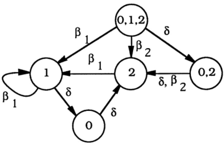
To illustrate ournotion of modelling, consider the system in Figure 2.1 and sup-pose that we wish to restrict its behavior to (a/,l)* by output feedback. In order to do this, we first specify L1 = a/l, as a primitive. For this example it is possible, essentially by inspection, to construct an L*C-restrictability compensator C : F* -4 U that is simpler than the one given in the proof of Proposition 2.12. Specifically, we can take C to be a function of the state of an automaton, illustrated in Figure 3.1, constructed from the observer for the original system simply by deleting the events which the compensator disables. The initial state of this system, as in the observer, is (0,1,2), and for any string s the compensator value C(s) is a function of the state of the modified observer. For example, if the first observed event is 6, the state of the system in Figure 3.1 is (1,2). In the original DEDS of Figure 2.1 the event /1 would

3 CHARACTERIZING HIGHER-LEVEL MODELS 20

Figure 3.1: Illustrating the Compensator for Eventual LiC-Restrictability by Output Feedback

V1 U / u1

Figure 3.2: Model of Task 1

be possible from state 0; however, as illustrated in Figure 3.1, we disable /3 so that the next observable event will either be 6 (from 0) or P2 (from 3 after the occurrence of a from 2). It is not difficult to check that the closed loop system Ac is eventually L*C-restricted, and thus the language eventually generated by Ac can be modelled at a higher level by the automaton in Figure 3.2 for which ,bl represents an occurrence

of al.

In order for this automaton, with ,1k observable, to truly model Ac, it must be true that we can in fact detect every occurrence of a/1 in Ac, perhaps with some initial uncertainty, given the string of observations of Ac. For example, by inspection of

Figure 3.1, if we observe i1, we cannot say if a/l1 has occured or not, but if we observe i1P1, we know that a/l1 must have occured at least once. Likewise, P2/1

corresponds to one occurrence of -a,1, 65/32/1S /1 - corresponds to -two occurrences of

/31l, etc. In general, after perhaps the first occurrence of ll, every occurrence of /1 corresponds to an occurrence of a/I and therefore, we can detect occurrences of '1 from observations in Ac. The definition we give in this section will then allow us to conclude that the automaton in Figure 3.2 models the closed loop system Ac.

To begin our precise specification of higher-level models, let us first introduce a function that defines the set of strings that corresponds to a primitive: Given alpha-bets E' and E, and a map He, : E- 2-*, if for all o E E' He(a) is a collection of finite length strings, then we term He a primitive map. Here a E E' is the macroscopic event corresponding to the set of tracking strings H(or) in the original model. We al-low the possibility that several strings may correspond to one macroscopic primitive to capture the fact that there may be several ways to complete a desired task.

We will require the following property:

Definition 3.1 A primitive map He is termed minimal if for all, not necessarily dis-tinct, al, a2 E E' and for all s E He('l), no proper suffix of s is in He(or2). 0

Given a primitive map, we extend it to act on strings over E' as follows: We let

He(e) = c and He(sa) = He(s)He(a), where s is a string over Y' and a is an element of E'. Also, He(s)He(cr) is the set of strings consisting of all possible concatenations of a string in He(s) followed by a string in He(a). We use the same symbol to denote

He and its extension to (E')*

Proposition 3.2 If He is minimal then for all distinct r1, r2such that rl, r2$ e, Jrx I<

3 CHARACTERIZING HIGHER-LEVEL MODELS 22

Proof: Assume the contrary, and let s E -*He(rl)n -*He(r). 2 Also let al (respectively,

0 2) be the last event in r1 (respectively, r2). There are two cases here: First, suppose

that al f or2. Then, there exist distinct pl E He(oi) and P2 E He(cr2) such that both

pi and P2 are suffixes of s. Assume, without loss of generality, that Ip I <

IP2

1, then pi is also a suffix of p2. But then, H, cannot be minimal. Now, suppose that 01 = 02. Thanks to minimality, among all elements of He(al), only one string, say p can be a suffix of s. Let s' be that prefix of s such that p = s/s'. Then, repeat the previous steps using s', and all but the last elements of rl and r2. Since rl and r2are distinct,

and r1 is not a suffix of r2, Ol will be different from 02 at some step and then we will

establish a contradiction. Therefore, E*He(ri) n E*He(r2) = 0. i

The following result states that we can concatenate minimal primitive maps while preserving minimality:

Proposition 3.3 Given minimal H1 : 2 --+

2E

; and H2 : E3 -- 2E2, if we define

H3 · 3 -+ 2E; so that H3(o) = H1(H2(a)) for all a E

S3,

then H3 is a minimal

primitive map. Here, since H2(a) is a set of strings, H1(H2(a)) is the set of strings

resulting from applying H1 to each string in H2(oJ).

Proof: Assume contrary, then there exists,

cl,0o

2 E "3, s E H3(al), and a suffix r of s so that r E H3(cr2). Let s' E H2((al) and r' E H2(0o2) such that s E Hl(s') and r E Hl(r'). Then, by minimality of H2, r' cannot be a suffix of s' and s' cannot be

a suffix of r' either. Also, since r is a suffix of s, s E E1HI(r'). Then, thanks to Proposition 3.2, H1 cannot be minimal, and we establish a contradiction. Therefore,

H3 must be minimal. O

Now, let us proceed with defining our notion of modelling. In particular, given two automata A = (G, f, d, h, t) and A' = (G', f', d', h', t'), we wish to specify when

A' is an He-model of the system A, where He: E' -E is a minimal primitive map. Two important properties that we will require of our models are the following:

1. Restrictability: We will require that if we can restrict the behavior of the macro-scopic model to some complete language L C E'*, then we can also restrict the original system to He(L)c. Note that we have defined L over E', instead of E'. Roughly speaking, we have done this since if all languages of interest are over the higher-level tracking alphabet E', then we can perhaps choose a simpler macroscopic model completely over E'. However, the alphabet -' will still be useful in defining different levels of modelling (see Proposition 3.6).

2. Detectability We will also require that for any lower-level string s in L(A) such that t(s) is in He(p) for some string p in the macroscopic system,

(a) we can reconstruct p, after some delay, using the lower-level observation

h(s) of s, and

(b) for any string r so that s is a suffix of r, the reconstruction acting on h(r) results in a string that ends with the reconstruction of h(s).

Note that minimality implies the following: If we let He-'(t(s)) denote the set of strings p E E'* such that t(s) E He(p), then, thanks to minimality, H- 1(t(s)) is single valued. Thus, in order to satisfy the first condition of detectability, we need to be able to reconstruct Hel(t(s)) from h(s). The second condition deals with the issue of start-up. Specifically, in our framework of eventual restrictability, we allow for the possibility of a transient start-up period in which the lower-level may generate a short tracking event sequence that does not correspond to any primitive. What (b) requires is that the reconstruction can

3 CHARACTERIZING HIGHER-LEVEL MODELS 24

recognize and "reject" such finite length start-up strings.

Definition 3.4 Given two DEDS A and A', and a minimal primitive map He: '

2? , we say that A' is an He-model of A if there exists a map H, : F* -, C'* and

an integer nd such thai4:

1. Restrictability: For all complete L C l'* such that A' is eventually L-restrictable,

A is eventually He(L)C-restrictable by output feedback.

2. Detectability: For all s E L(A), such that t(s) E He(p) for some p E L(A'),

(a) p E (E' U {c})ndHo(h(s)), and

(b) for all r E >*s, Ho(h(r)) E E'*Ho(h(s)).

Note that this concept of modelling provides a method of both spatial and temporal aggregation, as we will see, since A' may frequently be constructed to have many fewer states than A and sets of strings in A can be represented by a single event in

A'. For example, all states in Figure 2.1 are represented by a single state in Figure

3.2, and call is represented by 'l.

The following result, which immediately follows from Definition 3.4, states that the concept of modelling is invariant under compensation:

4_{We have chosen in our definition to look at the larger class of macroscopic languages to which} A is eventually restrictable by full state feedback, rather than only with output feedback. All of our results carry over if we use this weaker notion of restrictability at the higher level. Similarly in our definition of detectability we have required the stronger condition that from lower level observations, we can reconstruct the entire upper-level event trajectory, not just the part in F'. Again, we can carry all of our development over to the weaker case. As we will see, this stronger definition suffices for our purposes

Proposition 3.5 If A' is an He-model of A then for any compensator C' : I* -- U' for A', there exists a compensator C: r* -, U for A such that Al, is an He-model

of Ac with the same Ho.

L

In general, we may be interested in several different levels of aggregation. Thus, we need the following result which states that a higher-level model also models au-tomata at all lower levels:

Proposition 3.6 Given the automata A = (G, f, d, h, t), A' = (G', f', d', h', t'), and

A" = (G"',

f",

d", h", t"), and minimal primitive maps He : E' -+ 2-" and H ' _{: -k j}

2'*, so that A' is an H'-model of A with H' and A" is an H"-model of A' with

H", define r : · ' - 2-'- so that r(a) = oa(' U {e})lx'l for a E -' and define

He: E" - 2- as He(p) = He(r(H''(o))) for o E E". Then,

1. He is a minimal primitive map.

2. A" is an H,-model of A with Ho(s) = H'(h'(Ho(s))) for all s E r*.

Proof: 1. Clearly, xr is a minimal primitive map. Then, by Proposition 3.3, He is also a minimal primitive map.

2. Restrictability: If A" is eventually L-restrictable, then A' is eventually H,"(L)C-restrictable by output feedback -+ A' is eventually H' (L)c-H,"(L)C-restrictable -- A' is

even-tually 7r(H'(L)C)-restrictable - A is eventually He(L)C-restrictable by output

feed-back.

4 AGGREGATION 26

4 Aggregation

In this section, we use the concept of modelling of the previous section to present an approach for the aggregation of DEDS. What we have in mind is the following paradigm. Suppose that our system is capable of performing a set of tasks, each of which is a primitive as defined in the previous section. What we would like to do is to design a compensator that accepts as inputs requests to perform particular tasks and then controls A so that the appropriate task is performed. Assuming that the completion of this task is detected, we can construct a higher level and extremely simple standard model for our controlled system: tasks are requested and completed. Such a model can then be used as a building block for more complex interconnections of task-oriented automata and as the basis for the closed loop following of a desired task schedule.

In the first subsection we define tasks and several critical properties of sets of tasks and their compensators. Roughly speaking we would like tasks to be uniquely identifiable segments of behavior of A that in addition do not happen "by accident" during task set-up. More precisely, we introduce the notion of independence of tasks which states that no task is a subtask of another (so that all tasks describe behavior at roughly the same level of granularity) and the notion of a consistent compensator, which, while setting up to perform a desired task, ensures that no other task is completed. With such a set of tasks and compensators we can be assured that a desired task sequence can be followed, with task completions seperated by at most short set-up periods. In Section 4.2 we discuss the property of task observability, i.e., the ability to detect all occurrences of specified tasks. In Section 4.3 we then put these pieces together to construct a special higher-level model which we refer to as

task standard form.

4.1 Reachable Tasks

Our model of a task is a finite set of finite length strings, where the generation of any string in the set corresponds to the completion of the task. Let T be the index set of a collection of tasks, i.e., for any i E T there is a finite set Li of finite length strings over E that represents task i. In our development we will need a similar but stronger notion than that of minimality used in the previous section. We let LT = UiETLi and define the following:

Definition 4.1 Given T, we say that T is an independent task set if for all s E LT, no

substring of s, except for itself, is in LT. I

Then when we look at a tracking sequence there is no ambiguity concerning what tasks have been completed and which substring corresponds to which task. Note that if T is an independent set, then the minimal recognizer (AT, XO) for all of LT has a single final state xf, i.e., all strings in LT take x0 to xf, and Xf has no events defined

from it (since LT is a finite set). Furthermore, for each i E T, the minimal recognizer (AL', XLi ) also has a single final state x Li which has no events defined from it.

Let us define a second task L2 = aQ2 in addition to the task L1 = a3l for the example in Figure 2.1. Note that this system is in fact eventually L`C _and L>C-restrictable. We term such tasks reachable:

Definition 4.2 A task i E T is reachable if A is eventually Lc-restrictable. T is a

4 AGGREGATION 28

Definition 4.3 Task i E T is reachable by output feedback if A is eventually LC-restrictable by output feedback. T is reachable by output feedback if each i E T

is reachable by output feedback. I

Given a task i E T that is reachable by output feedback, let C : r* - U be an Lc-restrictability compensator. Consider the possible behavior when we implement this compensator. Note that states in Eo(Lc), as defined in Section 2.10, are guaranteed to generate a sublanguage of LC in the closed loop system. However, for any other state x E Z, although we cannot guarantee that LC will be generated given the particular knowledge of the current state of the system (i.e., given that the system is in some state in x), it may still be possible for such a string to occur. Furthermore, in general, a string in Lj, for some other j, may be generated from a state x E x before the trajectory in O reaches Eo(L*c). If in fact a string in Lj is generated from some x E x, then task j will have been completed while the compensator was trying to set-up the system for task i. Since this is a mismatch between what the compensator is trying to accomplish and what is actually happening in the system, we will require that it cannot happen. We define this property as follows (we state the definition for recurrent observer states, allowing for mismatch for a bounded number of transitions at the overall start-up of the system):

Definition 4.4 Given a reachable task i E T and an LTc-restrictability compensator

Ct, Ci is consistent with T if for all x. - Zr n Eo(L*c), for all x .E.., and -for all s E L(Ac, x), t(s) V LT.

Now, let us consider testing the existence of and constructing consistent restrictability compensators. Note that we only need to worry about forcing the trajectory in O into

the behavior can be achieved by the compensator defined in the proof of Proposition 2.12. First, we need a mechanism to recognize that a task is completed. Thus, let

(AT, x0) be a minimal recognizer for LT with the final state Xf. Let XT be the state space of AT.- Since not all events are defined at all states in XT, we do the following: we add a new state, say state g to the state space of AT, and for each event that is not previously defined at states in XT we define a transition to state g. Thus if AT enters state g, we know that the tracking event sequence generated starting from x0o and ending in g is not the prefix of any task sequence. Also, to keep the automaton alive, we define self-loops for all events in E at states g and Xf. Let AT be this new automaton. Given a string s over -, if s takes xo to g in AT then no prefix of s can be in LT. If, on the other hand, the string takes xo to xf then some prefix of this string must be in LT. Now, let O' = (G', w', v') be the observer for A 11 AT. We let the state

space Z' of O' be the range of initial states

Z0 = {P x {xo}IP C Z)} (4.1)

i.e., Z' = R(O', Zo). Let p : Z' -- Zr be the projection of Z' into Z,, i.e., given E Z', p() = U(X,, 2)ei{xl}. Also, let E' =

f{

E Z'lp( ) E Eo(Lc)}. Our goal

is to reach E' from the initial states ZO while avoiding the completion of any task. Once the trajectory arrives at E'ofurther behavior can be restricted as desired. So, we remove all transitions from states in E' and instead create self loops in order to preserve liveness. Let O" = (G', w", v") -represent the modified automaton. Let us now consider the set of states in which we need to keep the trajectory. These are the states that cannot correspond to a completion of any task. Thus, we need to keep the trajectories in the set

4 AGGREGATION 30

Let V' be the maximal (f,u)-invariant subset of E', and let KVI be the corresponding A-compatible and minimally restrictive feedback. In order for a consistent compen-sator to exist, ZO must be a subset of V'.- Assuming this to be the case, we need to steer the trajectories to E'o while keeping them in V'. Therefore, we need to find a feedback K": Z' -* U so that Z' is E -pre-stable in O. Uand so that the combined feedback K: Z' -- U defined by

K(Z) = KV'(p) n K"(8) (4.3)

for all z E Z' is A-compatible. The construction of such a K, if it exists, proceeds much as in our previous construction in Section 2. Thanks to the uniqueness of

Kv', if we cannot find such a feedback, then a consistent restrictability compensator

cannot exist. In the analysis in this paper, we assume that consistent compensators exist. That is, we assume that for each task ZO C V' and K exists.

Finally, let us outline how we put the various pieces together to construct a con-sistent compensator Ci for task i: Given an observation sequence s, we trace it in O starting from the initial state {Y}. Let x be the current state of 0 given s. There are three possibilities:

1. Suppose that xi Zr and the trajectory has not entered Eo(LC) yet. Then, we use 0 and an Eo(L*C)-pre-stabilizing feedback to construct Cl(s) as explained in the proof of Proposition 2.12.

2. Suppose that x E Zr and the trajectory has not entered Eo(LC) yet. Then, we use the observer 0" and the feedback K defined above. In particular, let x' be the state in the observer 0 into which the trajectory moves when it enters Z, for the first time, and let s' be that prefix of s which takes {Y} to x' in 0. Then,

we start 0" at state V' x xo and let it evolve. Suppose that s/s' takes x' x xo to 2 in 0" then

Ci(s) = (v"(z) n K(Z)) U (v"(Z) n a) (4.4)

3. When the trajectory enters Eo(Lc), we switch to using O(L*c) and the (f,u)-invariance feedback KLc. Ci(s) in this case can be constructed as explained in the proof of Proposition 2.12.

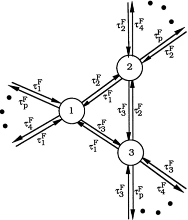
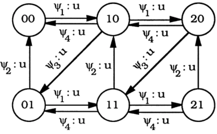
In order to develop a complete higher-level modelling methodology, we need to describe explicitly an overall compensator which responds to requests to perform particular tasks by enabling the appropriate compensator CQ. Given a set of p tasks T, reachable by output feedback, and a task i E T, let Ci : F* -- U denote the compensator corresponding to task i. The compensator C that we construct admits events corresponding to requests for tasks as inputs and, depending on the inputs, C switches in an appropriate fashion between Ci. In order to model this, we use an automaton illustrated in Figure 4.1, which has p states, where state i corresponds to using the compensator Ci to control A. For each i, r7f is a forced event, corresponding

to switching to C0. Let IT = {rlF,..., TF} and UT = 2"DT. The input to C is a subset

of (iT, representing the set of tasks which are requested at present. The compensator responds to this input as follows: Suppose that C is set-up to perform task i. There are three possibilities: (1) If the input is the empty set, then C disables all events in

A, awaiting future task requests; (2) if the input contains rF, then C will not force

any event but continue performing task i (thereby avoiding an unnecessary set-up transient); (3) Finally, if the input is not empty but it does not contain rF, then C will force one of the events in this set. At this level of modelling, we do not care which event C decides to force. Thus, we define C : UT x r* - U X rT so that given an input

4 AGGREGATION 32 2 t4 i FS4 F

ZI~~-

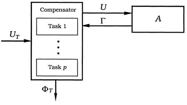
zz2 F 1 F ICF A zi F~~~~~ zlr3~~~~'C 2F 'CZ U

Compensator U

Task 1

UT

Task p

(DT

Figure 4.2: Block Diagram for Ac

in UT, C chooses the appropriate input (E U) to A and generates the forced events (E I(T) as explained above. If the action of C corresponds to a switch from one task to another, the compensator Ci is initialized using the approach described previously. Specifically, suppose that the observer is in state i right before rF is forced. Consider the three cases described previously for Ci: If x i Zr and x ~ Eo(Lc), then we use

O starting from the initial state x and an Eo(Lc)-pre-stabilizing feedback. If x E Zr and x ~ Eo(L!c), then we start 0" at state x x xo and use the compensator described previously to drive the system to the desired set of states. Finally, if x E

Eo(L),-L*C Lrc

then we start O(Luc) at state xo x x, where x0o is the initial state of the minimal

recognizer for L_ic, and we use the (f,u)-invariant feedback KL i. A block diagram for

4 AGGREGATION 34

4.2 Observable Tasks

In this section, we define a notion of observability for tasks which allows us to detect all occurrences of a given task. Consistent with our definition of detectability, we define task observability after an initial start-up transient. Specifically, we focus on detecting occurrences of tasks from that point in time at which the observer enters a recurrent state. One could, of course, consider the stricter condition of observability without any knowledge of the initial state, but this would seem to be a rather strong condition. Rather, our definition can be viewed either as allowing a short start-up period or as specifying the level of initial state knowledge required in order for task detection to begin immediately (i.e., we need our initial state uncertainty to be confined to an element of Zr).

Definition 4.5 A task i E T is observable if there exists a function IZ: Zr X L(O, Zr)

{e,

OF'} so

that for all

x E Zr

and for all

x E

x,

I

satisfies

1. I(x, h(s)) = · bF for all s E L(A, x) such that s = PlP2P3 for some P1,P2,P3 E *

for which t(p2) E Li, and

2. I(x, h(s)) = e for all other s E L(A, x).

A set of tasks T is observable if each i E T is observable. L

Since we assume that tasks are reachable throughout this paper and will use task observability only in conjunction with task control, we will construct a test for the observability of task i assuming that it is reachable and that we are given an L*c-restrictability compensator Ci which is consistent with T. Furthermore, thanks to consistency, we only need to construct I for x

E

Eo(Lc) and for strings s such

but with a self-loop at the final state xf ' for each oa E -. Now, let Q = (GQ, fQ, dQ),

with state space XQ, denote the live part of A'i 1. A, i.e., XQ is the set of states x

in XL, x X so that there exists an arbitrarily long string in L(A', 11 A, x). In fact,

note that for each x E X such that (XL',x) E XQ, there exists s E L(A,x) so that t(s) E Li. Finally, let OQ = (FQ, WQ, VQ) be the observer for Q so that the state space ZQ of OQ is the reach of

ZQO = U ({xLi } x;)

n

XQ

(4.5)

5EEo(L*c)

in OQ, i.e., ZQ = R(OQ, ZQo). Note that if i is observable, then the last event of each

string in Li must be an observable event. Assuming that this is the case, let

EQ = {: E ZQI3(x, y) E : such that x = xL'} (4.6)

Given the observations on Aci let us first trace the trajectory in the observer 0. At some point in time, O will enter some state x e E (L*c). When this happens we know that the system starts tracking task i. At this point, let us start tracing the future observations in OQ starting from the state ({xL' } x x) n XQ. This trajectory will enter some z E EQ at some point in time. At this point, we know that task i may have been completed. However, for task observability, we need to be certain that task i is completed whenever it is actually, completed. Thus, for an observable task, it must be true that for all ] E EQ and for all (x,y) E z, x = xf'. In this case we can define I to be e until the trajectory in OQ enters EQ and

/OF

from that point on Precisely stated, we have shown the following:

Proposition 4.6 Given a reachable task i E T and an Lc-restrictability

4 AGGREGATION 36

observable event, and (2) for all z E EQ and for all (x, y) E ,, x = xL' then task i

is observable in Ac,.

The procedure explained above allows us to detect the first completion of task i. Detecting other completions of task i is straightforward: Suppose that 0 enters the state y when OQ enters EQ. Note that g e Eo(L!c). At this point we detect the first occurrence of task i and in order to detect the next occurrence of task i, we immediately re-start OQ at state XoLi x g n XQ. The procedure continues with each entrance into EQ signaling task completion and a re-start of OQ. Note that the observer O runs continuously throughout the evolution of the system. Let D! : r*

{e, ,bF) denote the complete task detector system (which, for simplicity, assumes an

initial observer state of {Y}). We can think of D* as a combination of three automata: the observer 0, the system OQ which is re-started when a task is detected, and a

single one-state automaton which has a self-transition loop, with event O'F, which

occurs whenever a task is detected. This event is the only observable event for this system. Note that both the OQ re-start and the O/F transition can be implemented as forced transitions.

Finally, in the same way in which we constructed C from the Ci, we can also define a task detector D from the set of individual task detectors Di. Specifically, if

C is set at Ci initially, D is set at Di. Using the output AT of C, D switches between Di. For example, if D is set at Di and rjF is forced by C, then D switches to Dj. The

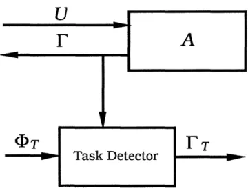
output of D takes values in rT = {bl,... , OF }. A block diagram for D is illustrated in Figure 4.3.

V

A

OT IFT

Task Detector

Figure 4.3: Task Detector Block Diagram

4.3 Task-Level Closed Loop Systems and Task Standard Form

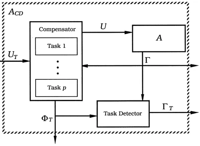
Using the pieces developed in the preceding subsections we can now construct a task-level closed-loop system as pictued in Figure 4.4. The overall system is ACD= (GCD, fCD, dCD, tCD, hCD) where

GCD = (XCD, U rT, UT, ArT) rr UIT U FT, u , (4.7)

Note that 'T and rT are both observable and rT is observable. Also, we include

OT

in the tracking events to mark the fact that the system has switched compensators. This is important since following the switch, we will allow a finite length set-up. Also, since it does not make much sense in practice to force a switch to another compensator while the system is in the middle of completing a task, we impose the-restriction that events in ~1_{T can only be forced right after a task is completed. Since we require}

4 AGGREGATION 38 ~sll~trvers5trs1trs1trsssssf trl/t~s~~///-/f/Jrf ff sf fsssfs

AcD

i

-0

Compensator __ i Task 1

A

fuT -0 ~ Task p

l

rr

TTask Detector

restriction. Then, ACD can only generate strings s such that

t(s) E ( U {(}) t_{(LL U... U L;)(He(r)LI U... U He(Tp)L;)*}

where nt is the maximum number of tracking transitions needed until 0 enters the set of recurrent states in Eo(LC) for each i E T.

The higher-level operation of this system consists of the task initiation commands,

AT and the task completion acknowledgements, rT. The input UT indicating what

subset of tasks can be enabled can be thought of as an external command contain-ing the choices -of subsets of q)T to be enabled. The use and control of this command involves higher-level modelling or scheduling issues beyond the purely task-level con-cept. What we show in this section is that the task-level behavior of ACD can in fact be modelled, in the precise sense introduced in Section 3, by a much simpler automa-ton ATSF = (GTSF, fTSF, dTSF) illustrated in Figure 4.5 where all the events are controllable and observable, i.e.,

GTSF = (XTSF, ETSF, DTSF = ETSF, rTSF = ETSF) (4.8) We are not concerned with defining the tracking events of ATSF since this alphabet is are not of concern in our main result below. We term ATSF the task standard form.

Let us first define He. We first define He(e) = e and He(4bi) = Li. Note that, thanks to the independence of T, for any pair of not necessarily distinct tasks i and j, no suffix of string in He(4i) can be in He(0bj). Defining He(ri) is more tricky. There.

are two issues:

1. We need to take into account the fact that the closed loop system does not generate strings in Li immediately after C switches to Ci. In particular, if we assume that O is in a recurrent state when C switches to Ci and if we let n,

4 AGGREGATION 40 9 4 02 *) 2 '-2 '1 0 'T3 Z4 0·a