Development Pattern and Prediction Error for the Stochastic Bornhuetter-Ferguson Claims Reserving Method

FOR THE STOCHASTIC BORNHUETTER-FERGUSON CLAIMS RESERVING METHOD

BY

ANNINA SALUZ, ALOIS GISLERAND MARIO V. WÜTHRICH

ABSTRACT

We investigate the question how the development pattern in the Bornhuetter-Ferguson method should be estimated and derive the corresponding conditional mean square error of prediction (MSEP) of the ultimate claim prediction. An estimator of this conditional MSEP in a distribution-free model was given by Mack [9], whereas in Alai et al. [2] this conditional MSEP was studied in an over-dispersed Poisson model using the chain ladder development pattern. First we consider distributional models and derive estimators (maximum like-lihood) for the development pattern taking all relevant information into account. Moreover, we suggest new estimators of the correlation matrix of these estimators and new estimators of the conditional MSEP. Our fi ndings supplement some of Mack’s results. The methodology is illustrated at two numerical examples.

KEYWORDS

Claims Reserving, Bornhuetter-Ferguson Method, Mean Square Error of Pre-diction, Claims Development Pattern.

1. INTRODUCTION

The chain ladder (CL) and the Bornhuetter-Ferguson (BF) method [3] are still the most frequently used claims reserving methods in practice. For both meth-ods it is assumed that there exists a development pattern gj, which is the same for all accident years. For the BF method there are, in addition compared to the CL method, given estimates mi of the expected ultimate claim of each accident year i, and the BF reserve of accident year i is obtained by multi-plying mi with the ‘still to come percentage’ of accident year i according to the development pattern gj. Thus, one essential difference between the CL and the BF philosophy is that the BF method incorporates mi in the reserve estimate. Often, the CL development pattern is used for the development pattern in the

280

BF method. However, this is not consistent with the BF philosophy, as the CL development pattern disregards any information contained in the mi’s.

Originally, both methods were established as purely pragmatic methods without an underlying stochastic model. Such a pragmatic approach allows to determine a point estimate of the claims reserve. However, in order to assess the uncertainties in this point estimate one needs an underlying stochastic model.

For the CL method Mack [8] presented such a stochastic model and a corresponding estimator for the conditional mean square error of prediction (MSEP) in 1993. For the BF method such models and estimators are com-paratively new. In 2008, Mack [9] introduced a distribution-free model under-lying the BF method and suggested estimators for the corresponding MSEP. Estimators of the MSEP for models related to BF were already derived earlier as, for instance, in England-Verrall [5] or in Neuhaus [10]. However, Mack’s model is probably the most general distribution-free model underlying the BF method. But this generality has also a drawback, namely, that many results in Mack [9] cannot be obtained in a stringent mathematical way and that one has to resort to pragmatic considerations and approximations.

Another approach was used by Wüthrich-Merz [13] and by Alai et al. [2]. Both studied the conditional MSEP in an over-dispersed Poisson (ODP) model where the development pattern is estimated by the CL development pattern.

In this paper we investigate the question how the development pattern in the BF method should be estimated considering all relevant information and how the corresponding correlation matrix looks like. For this purpose we consider stochastic BF models with parametric model assumptions for incre-mental claims. In these models we are able to derive the maximum likelihood estimators (MLEs) as well as the correlation matrix of the MLEs and derive estimators of the corresponding conditional MSEP. In contrast to the usual approach in which the chain ladder development pattern is used, we implement the BF philosophy in the estimates of the development pattern by incorporating the a priori knowledge in this estimation. In our opinion the new estimates for the development pattern, the correlation matrix and the conditional MSEP should generally be used for the BF method.

Moreover, we show how the variance of the a priori estimates can be esti-mated from the data. Finally, we apply our methods to real data from practice.

ORGANISATIONOFTHEPAPER

In the next section we introduce the notation and data structure. In Section 3 we give the basic assumptions underlying the BF method and recall the model of Mack [9]. In Section 4 we introduce three distributional models under-lying the BF method and derive estimates for the conditional MSEP in these models. Conclusions and numerical examples are given in Sections 5 and 6. Technical proofs of the statements are provided in Appendix A.

2. NOTATIONAND DATA STRUCTURE

We denote the cumulative claims (cumulative payments or incurred losses) in accident year i ! {0, …, I } at the end of development year j ! {0, …, J} by

Ci, j > 0 and we assume that J # I. Let Xi, j = Ci, j – Ci, j – 1 denote the incremen-tal claims, where we set Ci, – 1 = 0. In the sequel it is also useful to defi ne

[k j i,j . X X 0 k I 0 j J i k 0 # # # # = ], =

/

, ,

In general we denote the summation over an index starting from 0 with a square bracket. We assume that all claims are settled after development year J and there-fore the total ultimate claim of accident year i is given by C_{i, J}. At time I we have information

DI = {Ci, j : i + j # I, j # J}, and our goal is to predict DI

c

= {Ci, j : i + j > I, i # I, j # J}. The outstanding loss liabilities for accident year i at time I are given by

Ri = Ci, J – Ci, I – i ,  I – J + 1 # i # I, (2.1) and the total outstanding loss liabilities of all accident years are given by

R_i.

R =

/

Ii= - +I J 1

Remark 2.1. The ‘true’ outstanding loss liabilities are given by formula (2.1) only if Ci, j denote cumulative payments. For incurred losses Ci, j the outstanding loss liabilities are given by

Ri = Ci, J – Ci, I – i + Ci, I – i – Ci,I-i paid

, (2.2) with Ci, j

paid

denoting the cumulative payments of accident year i up to devel-opment year j. Note that the additional term Ci, I – i – Ci,I-i

paid

is observable at time I and has no impact on the claims prediction problem and uncertainty. Therefore we only consider the outstanding loss liabilities as defi ned in (2.1). For incurred losses, (2.1) is often referred to as IBNR.

3. BF RESERVING METHOD 3.1. BF Reserving Method

The BF method goes back to Bornhuetter-Ferguson [3]. There are a priori estimates of the expected ultimate claim Ci, J given by

282

where ni denotes the premium of accident year i and where qi is an estimate of the expected ultimate loss ratio. The BF reserve is then given by

Ri = mi(1 – bI – i ), (3.2) where 1 – bI – i is the estimated still to come factor at the end of development year I – i. In this paper we assume that the estimates mi are independent of the observations DI, which is for instance the case, if these estimates represent an external expert opinion or if they come from a pricing which is mainly based on common statistics of pooled industry-wide data. Note that mi is identical to an a priori estimate of the ultimate claim Ci, J, but that it is not its current predictor, which at time I is given by

Ci, J = Ci, I – i + Ri = Ci, I – i + mi(1 – bI – i ).

3.2. Basic Assumptions Underlying the BF Method

From the fundamental properties of the BF method we derive some basic assumptions, which an underlying model should satisfy. These assumptions are motivated in Mack [9]. The independence assumption between the current claim amount Ci, I – i and the reserve estimate suggests that incremental claims within the same accident year i are independent. The independence between different accident years is a standard assumption which we also adopt here. Moreover, from the BF reserve estimate (3.2) it follows that a stochastic model for the BF method has to be cross-classifi ed of the type

E [Ci, j ] = mibj or equivalently E [Xi, j ] = migj , with = k=0

j

.

j k

b

/

g Since migj = (mic) (gj /c) for any constant c > 0, the param-eters mi and gj are only unique up to a constant factor. Without loss of gener-ality one can therefore assume that g0 + … + gJ = 1. The sequence (bj)j then denotes the (cumulative) development pattern and (gj)j is the (incremental) development pattern. Further, we assume that the a priori estimates mi are unbiased for E [Ci, J ]. Hence we make the following basic assumptions for a stochastic model underlying the BF method.

Model Assumptions 3.1. (Basic Underlying Assumptions)

BF1 Incremental claims Xi, j are independent and there exist parameters

m0, …, mI, g0, …, gJ, with

/

Jj=0gj=1 such that

E [Xi, j ] = migj , 0 # i # I and 0 # j # J.

Mack’s Model: In addition to Model Assumptions 3.1 Mack [9] makes the following variance assumption

Var(Xi, j ) = mi sj2. (3.3)

Remark 3.2. Note that Mack’s model is a distribution-free model for the BF method. Since it is a very general model several approximations are used to estimate the prediction uncertainties.

Alai et al. Model: In addition to Model Assumptions 3.1 Alai et al. [2] assume that incremental claims Xi, j are ODP distributed. Prediction uncertainty is then studied within a MLE and generalized linear model framework, but by using the CL development pattern.

3.3. Estimation of the Development Pattern

In order to estimate the BF reserve and its conditional MSEP we need to estimate the development pattern gj, 0 # j # J. In practice one often uses the CL development pattern j = [ [ C C ] ] I k k I k k 1 1 1 -- -- + f_k f , where f . k j J k k j J 1 1 1 g - = = = -, , k CL

%

-1

%

-1 (3.4)

However, the use of the CL development pattern is not consistent with the BF philosophy, as it disregards the information in the a priori estimates mi. If the

mi were known then the best linear estimate of gj under Model Assumptions 3.1 and under the variance assumption (3.3) would be

j [I-j j] [I-j X m , ] = g) _, with m[k] = i=0 i, k _m

/

_{0 # k # I. Therefore Mack [9] suggests initial estimates} j [I-j j] [I-j X , ] g) = _{m ,}

and then applies manual smoothing such that the fi nal estimators gj sum up to 1.

The above estimators are not the only ones consistent with the BF philosophy, and the restriction to linear estimators is possibly not optimal. An alternative estimator is obtained with the following reasoning: assume fi rst that we are given a full rectangle. Then an obvious estimator is

[ ] [ ] I I,j , . C X j = J g

284

Note that the gj automatically sum up to 1. As only the upper trapezoid DI is given, a natural idea is to replace the unknown Xi, j in the lower right tri-angle of DI by the BF predictors mi gj resulting in the following system of equations , , i i j j i i + + j J i I, -i l , . C C X j J 0 i I J l I i J i I J I i I j i I j I 0 1 1 0 1 m m # # = + = -= - + = - + = -= - + g g g ` j

/

/

/

/

/

(3.5)

In order to investigate different estimators and the corresponding conditional MSEPs more precisely we consider explicit BF models with parametric assump-tions for incremental claims Xi, j. All the models considered in the following will satisfy Model Assumptions 3.1 and the variance assumption (3.3). Hence they are all special cases of the model considered in Mack [9]. In these distribu-tional models we are able to derive estimates (MLEs) of the development pattern in a stringent mathematical way. Moreover, we fi nd explicit solutions for the correlation matrices of these estimators, which are needed to calculate the MSEP of the BF reserves. As we will see, in one of the models, the above estimator (3.5) turns out to be the estimator corresponding to the MLE, if we replace the unknown mi by mi.

4. STOCHASTIC BF MODELSBASEDON PARAMETRIC DISTRIBUTIONS

4.1. Over-dispersed Poisson Model with Constant Dispersion Parameter 4.1.1. Model

In Model Assumptions 3.1 we have specifi ed the basic assumptions of the BF model. In the following model we assume that the Xi, j follow an ODP distribu-tion with constant dispersion parameter.

Model Assumptions 4.1. (Over-dispersed Poisson Model)

P1 Incremental claims Xi, j are independent and there exist positive parameters f, m0, …, mI and g0, …, gJ with

/

Jj=0gj=1 such that Xi, j / f + Poisson (migj / f). In particular, we have

E [Xi, j ] = migj , Var(Xi, j ) = fmigj , where f is called dispersion parameter.

P2 The a priori estimates mi for mi = E [Ci, J ] are unbiased and independent from Xl, j for 0 # l # I, 0 # j # J.

Remarks 4.2.

– In the ODP Model the incremental claims Xi, j are required to be positive. – Disregarding the mi, that is considering data DI only, the MLEs for the claims

reserves and the development pattern are identical to the CL reserves and the CL development pattern gjCL, see for instance Hachemeister-Stanard [6], Mack [7] or Schmidt-Wünsche [12].

– Alai et al. [2] used a similar model to derive an estimate for the conditional MSEP in the BF method.

– Note that we have not made any assumption on the dependence structure between the mi’s.

4.1.2. Estimation of the Development Pattern

We estimate the development pattern with the MLE method. In order to calculate the MLEs we fi rst assume that the mi are known and then plug in the estimates mi. The MLEs are best calculated using Lagrange multipliers. Note that in the ODP case the log-likelihood function for Xi, j is given by

, ,

i j j j i j

f1 `X `logmi+logg j-migj-g(X ,f),

where g(·, f) is a normalizing function that does not depend on the parameters

mi and gj.

Remark 4.3. Multiplying the log-likelihood function by f, we observe that the MLEs for the gj’s do not depend on the dispersion parameter.

Neglecting the normalizing function g we obtain the Lagrange function with Lagrange multiplier k given by

, i j( j j 0 i L_D , _J, X log log j i 1 . i j I j J 0 I + - + -# + = g f,g k = m g ) m g k g ` j

/

` j e

/

o

Observe that the last term comes from the normalization requirement

j 1

j=0 = .

J _g

/

For the MLEs gj we obtain the following equations

, i j j j i D L X 0 i I j 0 I 2 2 - = -m -k = = _g , g

/

e o

and therefore we fi nd the solutions

[I-j]

= X[I-₊j] .

j

286

From the side constraint it follows that

j D L 1 0 j J 0 I 2 2 = - = = , k

/

g

which yields in view of (4.1) an implicit equation for k

[I-j]+ m [I-j] 1 X 0 j J 0 - = = k . , j

/

(4.2)

From equation (4.2) it follows that k is the root of a polynomial of degree J + 1. Since the gj need to be positive in the ODP Model and since m[I – j ] is

decreasing in j we have the constraint k ! (– m[ I – J ], 3). In this interval there is a unique solution k by monotonicity (cf. Remarks 4.6).

Remark 4.4. We do not use the partial derivatives with respect to mi. This is not necessary since we already have the a priori estimates mi and therefore do not want to use MLEs for the mi.

Then, we replace the true (unknown) mi by the estimates mi and obtain the estimators = [I-j] [I-j] m X j g _k + , , j (4.3) where k fulfi lls the implicit equation

0 j 1 . j J 0 = = -

/

g (4.4)

Theorem 4.5. The estimates (4.3) satisfy equations (3.5).

Proof. Observe that the gj’s defi ned in (3.5) satisfy the constraint j=0 j=1.

J _g

/

Therefore it is suffi cient to prove that the estimates gj defi ned in (4.3) satisfy j 0 j [ ]I i , i= - +I j 1 1 . X X j J [I j] g g m # # = -I , 0 + g , j

/

From equation (4.3) we have k =

j [I-j

g

X ],j

– m[I – j ] for 0 # j # J and conclude

j j j j 0 [I-j j], j [ ]I [ ]I [ ]I i [I-j = i= - +I j 1 , , , [ ]I _{[ ]} I . X X X X 1 1 g [ ] X I j ], g g m +k g = _{m + m} g = + m -I -0 0 0 g j e o

_f

_p

/

Remarks 4.6.

– If instead of mi the data of the fully developed rectangular was given, then the MLE of gj would be

[ ], [ ] I I j , j J X g = C MLE _,

and would not depend on the mi at all. This shows that in the ODP Model the MLEs are not linear in the observations Xi, j. Given DI, the mi’s appear in the MLEs only to the extent that the entries Xi, j in the lower right triangle are not known and fi lled up with the BF predictors mi gj.

– From Theorem 4.5 it follows that the estimators gj obtained by replacing the unknown mi in the MLEs gj by mi satisfy equations (3.5). However the easiest way of fi nding the solution of equations (3.5) is to calculate the estimators gj by means of equation (4.3). There we only need to calculate k, which can be done quite easily by starting with k = 0, that is with the raw estimators

_j [ ] [ ], I j I j -m j X g( )0 = ,

and then by increasing or decreasing k until the side constraint

f _j =1 j J 0 g = ( )k =

/

is fulfi lled. Note hereby that in the interval (– m[ I – J ], 3) the function f (k) is

strictly decreasing and consequently the side constraint f (k) = 1 has a unique solution. Of course bj is then estimated by bj = k=0gk,

j

/

0 # j # J, and

sat-isfi es bJ = 1.

– From the estimators (4.3) we also see how a mathematically founded smooth-ing from the raw estimators gj(0) to the adjusted estimators gj looks like in the ODP Model. If we write

j cj j

( )0

g = g

then the ‘correction factors’ cj are given by

_j m [ [ I j I j -m ] ] = . c k +

Since m[ I – j ] is decreasing in j, cj is decreasing in j for k > 0 and increasing for k < 0. For instance, if k < 0 then the correction factor is greater for the late development years than for the newer ones.

– Consider the effect of conservative a priori estimation. If we increase some of the a priori estimates mi then k is decreasing because of the side

288

constraint (cf. (4.3)-(4.4)). We denote the new estimates by mi

c_{, g}

j

c _{and k}c . For the change in the denominator of gj we then have

[I-k] [I-k] [I-j] [I-j 0 j<k J, c m _-m ₊k _-k m# _-m ₊k _-k # # ] , c c c

and because of the side constraint there must be an index 0 # l < J such that for all j # l < k we have

m[I-k]-m[I-k]+k -k#0# [I-j]-m[I-j]+k -k

c _m c _.

c c

It follows that gk c

$ gk for all k > l (in the tail) and for j # l we have gj c

# gj. This means that more weight is given to the tail and the effect of conservative a priori estimation is therefore reinforced by the estimates of the development pattern. Note that in the case where we only increase mi with i # I – J the estimates of the development pattern remain unchanged (cf. (3.5)).

– The quality of the BF estimators strongly depends on the quality of the a priori estimates mi. If gj

J j=0

( )0

/

_{deviates much from 1 and thus k deviates} much from 0, then this could be an indicator that the a priori estimates might be biased. As a further check one could estimate the development pattern and the reserves by disregarding the a priori estimates mi. In the OPD Model with a full development triangle or trapezoid the resulting MLEs are then identical to the CL estimates. If for most accident years the CL predictors for the ultimate claims were either higher or lower than the BF predictors, this would be a strong indicator that the a priori estimates mi might be biased and that one of the basic assumptions of BF is violated. Sometimes one then adjusts the a priori estimates mi (see e.g. the Cape Cod method in Wüthrich-Merz [13] or Radtke-Schmidt [11], which goes back to Bühlmann-Straub [4]). There is no problem to calculate the BF reserves with ‘a posteriori’ adjusted mi. But this means that the mi are no longer independ-ent of the data DI, which should be taken into account for the estimation of the MSEP and is beyond the scope of this paper.

– A tail development gJ + 1 can be incorporated by replacing the side constraint in the Lagrange function by _j=0 _j

J _g

/

_{= 1 – gJ + 1. The estimate gJ + 1} needs to come from outside together with an estimated covariance structure

Cov \_(g

J + 1, gj), 0 # j # J + 1, because there is no data available for the tail.

Finally, we need to estimate the dispersion parameter f. As in Wüthrich-Merz [13] we use Pearson residuals to estimate f. The Pearson residuals are given by

j j , i j i i = R_i, X -m g m g j ,

with E [R2i, j ] = f. To estimate Ri, j we replace mi and gj by estimates, but we need to be cautious here. We want to estimate the variance of the Xi, j and therefore we are only interested in the process variance term and not in the parameter

estimation error. The uncertainty of the external estimate mi is considered in a different step. As a consequence we have to estimate mi and gj from the data in order to obtain an estimate for f. We use the MLE method to gain data based estimates for mi and gj. As mentioned in Remarks 4.6 in the case of ODP data in a full triangle or trapezoid the MLEs of mi and gj coincide with the CL estimates. Therefore we estimate Ri, j with

j j , i j , , i J i J -R C C X , i j g g = CL CL CL CL ,

where the CL development pattern gjCL was defi ned in (3.4) and where C =i JCL,

i, j= -I i

J-1 j.

C _I-i

%

f An estimate for f is then given by

f1 i+j#I i, I R = p e e -2 j D ,

/

(4.5) where | DI | is the number of observations in DI and where p = I + J + 1 is the number of estimated parameters.

In order to quantify the uncertainties in the BF predictors Ci, J and ,

i i= - +I J 1

I _C

J

/

_{we consider the conditional MSEP. Given information II , the} conditional MSEP of a predictor X of a random variable X is defi ned by

X ( 2 X X msep E[( _I I = - e e_I ) X ) I].

If in addition the predictor X is II -measurable we obtain 2 ( X X I I X msep Var (X ) ( [E X ] ) . I = e + e -eI ) I I

For the calculation of the conditional MSEP we therefore need to consider second moments and covariances of the estimates.

4.1.3. Covariance Matrix of the Estimated Development Pattern

In this section we consider the estimation of the covariance matrix of the gj’s. A well-known result from statistics is that MLEs are asymptotically unbiased and multivariate normally distributed. Moreover, the asymptotic covariance matrix is given by the inverse of the Fisher information matrix. By defi nition, the entries of the Fisher information matrix H(g) are given by

, j D D j k k I I ( , 0 , 1, H E 2l l #j k#J 2 2 2 = -g) = _{g g} G where l_D

I is the log-likelihood function. In the ODP case the log-likelihood

290 , i j j , i J j j j X j D _f f log log log log l X r 1 1 _{1 1} J J i j I i i I J j J i j J 0 1 1 0 0 1 0 1 I = + + + - - + # # -+ = -= -= -g _i i , m -,f, m g g g m g m g ^ ` ` e e e e h j j oo oo

/

/

/

/

where r contains all remaining terms, which do not depend on g = (g0, …, gJ – 1). Note that the last line of the above equality comes from the normalizing con-dition

/

Jj=0g_j=1. For 0 # j # J – 1 we obtain the diagonal elements

, , , , i j i i j i , j [I-j] [I-J] j j i i j j j 2 2 D f f f f f f f f Var Var . H E l E X X X X 1 1 1 1 1 1 j i I i I J J J i I i I J J J i I i i I J J i J j j j 2 0 0 2 0 0 0 0 I 2 2

g

g

g

g

= = - -= + = + = + = -= -= -= -= -= -m m m m m -m (g _{g g} g g g ) e e e e e e o o oo o o

>

H

=

/

/

G

/

/

/

/

(4.6)

Analogously, for 0 # j < k # J – 1, we have the off-diagonal terms

( _{k, j,} j J D D [I-J] f ) . g H _{j k} E k I I 2 2 2 2 = = = m l l g ( _{g g} H )g = G (4.7)

Hence, we write the Fisher information matrix as follows

J J J J J 1 -[I-J] f ( 1 . H 1 1 1 1 1 1 1 1 _RJ J [ ] [ ] [ ] [ ] [ ] [ ] I J I I J I I J I J 0 1 1 1 g g j g h ! = # m m m m m m -- + m h h / / / / / / g + + ) + g g g g g g g J L K K K K K K N P O O O O O O

For the entries of the inverse of the Fisher information matrix we obtain (see Appendix A) l , j { k -j / k= 1 [I-l] } j=k [I-j] [I-k] f ( ( ) / , 0 j k, J 1. l 1 0 # # -= m _{g m} g m J H g) g

f

p

/

(4.8)

We now assume that the mi are close to the true mi and therefore the covari-ances Cov (gj, gk) are close to the covariances of the true MLEs gj (cf. (4.1)). With the asymptotic MLE approximation we then obtain

j j, 1 -k ov ( , ) ( ( ) , C g g ._k H g)

and of course the covariances of gJ = 1 – j=0 j J-1_g

/

_{are obtained by linearity.} Replacing the parameters gj, f and m[I – j ] by their estimates gj (see (4.3)), f1 (see (4.5)) and m[I – j ] (see Model Assumptions 4.1) we arrive at the following

esti-mates for the covariances

j j / k k { , _m -[I-j] g } l=0 1 f ( ) , 0 , . Cov j k J [ ] [ ] l I l I k g g g m g m # # = -J j=k / t

f

p

\

/

(4.9)

This is clear for 0 # j, k # J – 1 and also holds for 0 # j, k # J. Note that j [ ] [ ] I j I j -m , = X j

g

)

are uncorrelated with variance j [I-j] m j f Var (

g

))= g

Hence the off-diagonal elements and the second term in (4.9) come from the side-constraint that the estimators have to sum up to one.

4.1.4. Conditional MSEP

In this section we derive estimates for the conditional MSEP of the BF predic-tors Ci,J = Ci,I – i + mi (1 – bI – i) and

/

I_i= - +_{I J 1}C_i,j under Model Assumptions 4.1. Let m_{1 = (m}0, …, mI ) and let II = s(DI, m1) denote the s-fi eld containing the information at time I. Due to the II-measurability of mi and bI – i we have

b b m , , i j i j , i J C i j I j e i , i I -i msep ( ) ( ) ( ) . E X E X j I J I i I j I i J i j I i J i I i 1 2 1 2 1 2 J m m = -= - + - -= - -= - + = - + -m g + I 1 1 g C I I f f f p p p

>

>

H

H

/

/

/

With the independence of the Xi, j and the defi nition

/

Jj= - +I i 1gj=1-b_I-_i we obtain 2 I-i b , i j , i J C i e , i I j= - +I i 1Var i I-i

b

msep ( ) (X ) ( ( ) )) .

Process Variance ( Estimation Error (EE ) i J i m = + - -m -I ( ) J 1 PV C 1 1

/

4 4 4 4424 4 4 443 14 4 4 4 4 4424 4 4 4 4 443

292

The process variance refl ects the randomness of the Xi, j and the estimation error describes the uncertainty in the parameter estimates.

Process Variance. For the estimation of the process variance recall that Var(Xi, j) = f migj according to Model Assumptions 4.1. If we plug in the parameter estimates we obtain the estimator

j , i j i ( ) f f ( b ). PV Var X j I i J j I i J i i I i 1 1 g = -= - + = - + -1 m m = = t t \

_/

\

_/

Estimation Error. Given II, the term ( mi (1 – bI – i ) – mi (1 – bI – i))2 is an unknown constant. In order to estimate this constant we rewrite it as follows

b b _i b _i I i I i I i I i - -- -2 i i + i i 2 _b -m i ( ) ( ) ( ) ( ) ( ) ( ) ( ) ( ) 2 1( ) ( ) ( ), i I i i i i I i I i I i I i I i I i 2 2 2 2 m m b b m m b - - - = - - + -= - - + - - -- - -- - - -m b m m m m m 1 1 1 1 b b b _ i _ i

and estimate the unknown terms ( mi – mi )2, ( bI – i – bI – i )2 and ( mi – mi ) ( bI – i – bI – i ) by taking the mean over all possible II, that is, we study the fl uctuation of mi

and bI – i around the true values mi and bI – i, respectively. If we neglect the

dependencies of the mi and the bj we obtain with the unbiasedness of the mi and the (approximate) asymptotic unbiasedness of the bj the following estima-tor for the estimation error

i 2 _b b _i ( ) ( ) ( ) EEi = 1- _I-_i Var m +m2Var _I-_i , \ \ \

where \Var( )m_i and \Var(b_I-_i) are estimates for the variances Var (mi) and

Var(bI – i), respectively. The variance of the bI – i is estimated using the Fisher

information matrix j b_{I-i k} ( ) Var Cov 0#j k, #I-i ( ,g g ,) = \

_/

\ _(4.10)

where the covariances \Cov(g g_j, _k) are given in (4.9).

It remains to estimate the variances of the a priori estimates mi. An actuary being able to deliver a priori estimates mi is often also able to make a statement about the precision of these estimates. In this case beside the mi’s there are also given a priori estimates of Var (mi). If this is not the case we show how Var (mi) can be estimated from the data. To this end we assume that the mi have a con-stant coeffi cient of variation CoVa(mi) / c and that the correlation Corr(mi, mk) can be estimated by e i k ( ) , and 0, else Corr n 0 i k I k <n n i k _{# #} = e -, i , m m

*

, -\ _(4.11) where 0 # n # I.

Remark 4.7. In the case where the premiums ni and the variances of the ulti-mate loss ratios are constant, we obtain the above formula for the correlation

Corr \_{( m}

i, mk) if the a priori loss ratios are estimated with a moving average of the ultimate loss ratios over n years (cf. Appendix A). Observe that we do not assume that the a priori estimates mi are independent.

In the numerical examples we will use formula (4.11) with n = 10, assuming that information more than 10 years ago does not contribute to the new fore-cast. We defi ne the aggregated claim amount at time I by

, i i, I J C I-i. C C i I J i I J I 0 1 = -= - + = +

/

/

The corresponding pure risk premium is given by

. b_I-_im [ ] E 1 I I i i I J i I J I 0 P = = = -= - + i C

/

m +

/

(4.12)

Moreover, we defi ne the observed loss ratio at time I by

I I I I I P P Q = = P P I I C C ,

where PI is obtained from (4.12) by replacing all mi by the a priori estimates mi. With a fi rst order Taylor approximation around PI we obtain

I P I P PI

[ / ] 1 and Var ( / ) V ( ),

E P _I . P _I . Co a2

and therefore with the independence of PI and CI we conclude that E [QI] . 1. For the variance Var(QI) we use the following general decomposition for the product of independent random variables X and Y

. Var (XY)=E X[ ] Var ( )2 Y +E Y[ ] Var ( )2 X +Var ( ) Var ( )X Y

Henceforth we have with the Taylor approximation

I I I

I I I P

Var (Q ).Var (C ) /P2+CoVa (2 P_I)+Var (C /P ) Var (P / _I).

Neglecting the last term and asserting positivity we arrive at the following estimator

I I

P P

( ) , ( ) ( )

Co aV _I =max 0 Var Q -Var C / I 2

,

2 _{& 0}

\ \ \ X

294 m s b b [ [ [ , _I J 2 j i I i i I-i , with / , 1 s P P Q f ( ( 1)

( ) with in the ODP Model

Var Var Q C C i I J I i i i I J I I I I i I J i I J I 0 0 1 m m m s = = = = -= - + = -= - + I I ] 2 ) = ] j . -= , + 2 2 , ] Q + t X \ X \

/

/

/

/

Note that if the mi were fully correlated then CoVa(mi) = CoVa(PI ). In general we obtain with the calculation provided in Appendix A

Corr ( b ( i - _i -P 2 I-i k i k b Va ( ) , Va ) , , max c 0 1 2 1 i I i I _{i k I} I i I k 2 2 0 2 0 < m m = # # = - - m m = b Co m 1 -Co m ) J L K K K _e _ N P O O O o i Z [ \ ] ] ] ] _ ` a b b b b

/

/

(4.13) where we set bj = 1 if j > J. The variance is then estimated by

( _i) c $ _i Var m = 2 m ,2

\ _(4.14)

where c2 _{is obtained from (4.13) by replacing the unknown CoVa}2 _(P

I ),

Corr (mi, mk) and the parameters by their estimates.

Thus, we have derived the following estimate for the conditional MSEP of

Ci, J :

Estimate 4.8. (MSEP single accident year) Under Model Assumptions 4.1 the conditional MSEP of the BF predictor Ci, J is estimated by

+ 2 b b -, i i j i C I( J) f ( ) (1 ) i Var ( ), msep Var 1 j I i J I i I i , i e + m = - + - -m m J 2 C = g I t \

_/

\ \

where \Var (b_I-i) is given in (4.10) and \Var( )m_i is given in (4.14). For the estimates mi, gj and f1 see Model Assumptions 4.1, equation (4.3) and (4.5), respectively. Our next goal is the derivation of an estimate of the conditional MSEP for aggregated accident years. We have

C C , , , , , , , , i i i i i i k C C J J J J J J k J J , , i i -i= - +I J 1 C C C msep msep ( ) . E E C C 2 i I J I i I J I i I J I I i I J I I J i k I I 1 1 1 2 1 1 < J I J I = = + - -e e # # = - + = - + = - + = - + - + I I C I I I e e ` ` o o j j

>

8

H

B

/

/

/

/

/

/

As above using the II measurability of bj and mi we obtain for i < k X b b , k , , , , i i k X b , i i J J k J J I-i I-k k I-k j C C Cov , ( ) ( ) ( ) ( ) . E C C 1 1 I j j I i J j I k J i I i k m m - - = + - - - -= - + = - + - m 1 1 m 1 b 1 I ` ` f _ _ j j p i i 8 B

/

/

With the independence of the incremental claims Xi, j we see that the covari-ance term is equal to zero and given II the last expression is an unknown constant. In order to estimate this unknown term we proceed as above and defi ne b b b b I-k -b i k i i k k , i k -I-i ( ) ( ) ( ) ( ) ( ) ( ) EE 1 1 1 1 1 1 k i I i k I k I i i I i I i I k I k I k m m m b m = - - -= - - - -- -- - - -m b m m m m b b , m -b ` _ ` ` ` _ _ _ j ij j ij i i which is estimated by b b - I-i -bI-k _{i k i} bI-k ( ) ( ) ( , ) ( , ), EEi,k= 1 1 Cov m m +m m_kCov _I-i \ \ \ where i k i k i k ( , ) ( , )

Cov m m = Corr m m Var^mhVar^m ,h

\ \ \ \ _(4.15) and j l b_I-_i I-k 1 , , Cov Cov I J i k I l I k j I i 0 0 # # = - + = -= -,b ( , ),g g ` j \

_/

_/

\ _(4.16) (see (4.14) and (4.9)).

Putting everything together we obtain the following estimate for the con-ditional MSEP:

Estimate 4.9. (MSEP aggregated accident years)

Under Model Assumptions 4.1 the conditional MSEP for aggregated accident years is estimated by b b , , i i - - _{i i} , i J C b J J I-i I-k I-i I-k , i C b k k i= - +I J 1 J C C (1 ) (1 )Cov( , ) Cov( , ) . msep msep 2 1 1 i I J I i I J I I J i k I 1 < I I m m = + + e e # # = - + = - + - + m m I Ie I` ` o j j \ \ \ \

/

/

/

/

Remark 4.10. In the literature one often calculates the conditional MSEP given DI instead of II. This corresponds to a different interpretation. If the mi

296

are considered as observations one should condition on II otherwise if the mi are considered as a priori information one should condition on DI. That is, in the latter case we are in a Bayesian framework, where mi are random variables with an a priori distribution and mi is the expected value of mi. In the fi rst case mi is treated as an ‘expert observation’. In the case where we condition on DI we obtain for single accident years

2 I-i b , i j , i J C i e I , i j= - +I i 1Var i I-i b D msep _D ( ) (X ) E ( ( ) )) . EE i J i m = + - -m -I ( J 1 PV C 8 1 B 1

/

4 4 4 4424 4 4 443 14 4 4 4 4 4 4 4 4424 4 4 4 4 4 4 4 443

In order to estimate the last term we consider the mean over all possible DI (we could also use this procedure when we condition on II and the resulting estimates differ slightly).

With the approximation E [mi(1 – bI – i)] . mi (1 – bI – i ) we obtain

b b b Var E b - -i i i i i i - i - _I-i I-i ( ) ( ) Var ( ) Var ( ( ) ) ( ) E E 1 I i I i I i m m m em m m . -= - + - -m 1 1 1 1 b 2 , ` `

_

j j i 8 8 8 B B B

and estimating the last term we obtain the following estimate for the estima-tion error b b i i i ( ) Var ( ) (1 ) Var ( ) . EEi = `m2+Var m j 1- _I-i + - _I-i 2 m \ \ \ \

We therefore have the additional term \Var ( ) Varm_i \(1-bI-i) in the estimation error. Similarly we have for aggregated accident years

b b

i( ) i( bI-i) k( I-k) ( bI- ) DI

EE_{i k,} =E8_m 1- _I-i -m 1- i_m 1- -m_k 1- _k i B,

which is estimated by

bI-i bI-k ( ,_{i k}) ( ,_{i k}) _{i k} (b ,b ) . EEi k, =`1- j`1- jCov m m +`Cov m m +m m jCov _{I-i I-k}

\ \ \ \

The resulting formulas for the conditional MSEP have the same form as the estimates derived in Mack [9] (but the estimates of the parameters and covariances are, of course, different).

4.2. General Over-dispersed Poisson Model 4.2.1. Model

In Model Assumptions 4.1 we have assumed that the dispersion parameter f is constant over all development years. The assumption of a constant dispersion

is quite restrictive and often not appropriate in practical applications. Therefore we consider in this subsection the general case, where the dispersion parameter varies between development years.

Model Assumptions 4.11. (General Over-dispersed Poisson Model)

GP1 Incremental claims Xi, j are independent and there exist positive param-eters f0, …, fJ, m0, …, mI and g0, …, gJ with

/

Jj=0gj=1 such that

Xi, j /fj + Poisson ( mi gj / fj ). In particular, we have

j i , , i j i j i j j f [ ] Var ( ) E X X = = m , , m g g

where fj is the dispersion parameter for development year j.

GP2 The a priori estimates mi for mi = E [Ci, J ] are unbiased and independent from Xl, j for 0 # l # I, 0 # j # J.

4.2.2. Estimation of the Development Pattern

As in Section 4.1 we estimate gj with the MLE method using Lagrange multi-pliers. The Lagrange function is given by

j i j, i j i j j J k D L , , _f1 X log log 1 i j I j J 0 0 I + - + -# + = g f,g k = m g m g g , ` j

/

` ` j j e

/

o (4.17) where k is the Lagrange multiplier. For 0 # j # J the MLE gj is the solution of

j , i j i j j D L f 0 X 1 0 i I j I 2 2 = - - = = -m k , g

/

e g o (4.18) and hence [I-j] + m , i j i j j j [I-j j], j f f f f / . X X 1 1 i I j i I j j 0 0 = + = = -= -k k / g m

/

/

(4.19)

Remark 4.12. Note that (4.19) has the same structure as (4.1) with respect to the normalized random variables Zi, j = Xi, j / fj.

With the side constraint we obtain the following implicit equation for k

[I-j] + m _j [I-j j], D L f f 1 X _/ j 0. j J 0 I 2 2 = - = = k k /

/

298

It remains to estimate mi and fj.

For mi we use the a priori estimates mi. In order to estimate the dispersion parameters fj we consider Yi, j = Xi, j / mi with

j , , i j i j j i i f Y j j Y and Var ( ) E 2 = = _m = _m [ ] g g s ,

where sj2 = fj gj. An unbiased estimate for sj2 is given by

, i j j mi Y -Y s _I1 _j ( ) , 0 j J j, I 0 i I j j 2 ! # # = - ₌ -, 2

/

_(4.20) with Yj i m i j, I j 0 = - _. [ i

=

/

m_{I- ]j} Y If J = I we use an extrapolation to obtain an estimate for s_J2_{, see Mack [8]. The dispersion parameter f}

j can then be estimated by j j j f = s_g 2 , t _(4.21)

where sj2 is obtained from sj2 by replacing the unknown mi’s by the a priori estimates mi and where

j j [I-j] j m , f f / / X [I j] g k = + -j , t t (4.22) with m j min f j J 0 [ k! _- 3 # # I-j , ] t

c ' 1 m given by the implicit equation

j [I-j] j m , f f 1 / / 0 X [I j] j J 0 k -+ = -= . j t t

/

Note that (4.21) is an implicit equation since ftj also appears in the equation for gj. If we plug in ftj = sj2 / gj in (4.22) we obtain

j j j j j / / X [ ] [ ], I j I j g g m s k g s = + -2 2 j ,

and solving for gj we get

j j [I-j j], X [I j] [I j] g = _m -k _ms - -. 2

With the side constraint j=0 j 1

J _{g =}

/

_{we arrive at the following explicit solution}

j l j [I-j j], [I-], l . X X 1 [ ] [ [ ] [ I j _lJ I I j I l l l J 0 0 g _m s m s m m = + -- ₌ -= l / / 2 2 ] ] e o

/

/

(4.23)

The cumulative development pattern is estimated by b =j k=0g_k, j

/

_{0 # j # J.} Remarks 4.13.

– For the case of a constant dispersion parameter f we cannot use the above estimation procedure for f. In that case sj2 / gj / f but sj2 / gj might not be constant over all j . Moreover, if f is constant over all development years, it does not make sense to consider the development years j separately for the estimation of f.

– The estimators (4.23) do not fulfi ll equations (3.5) anymore.

– Contrary to the ODP Model, the MLEs based only on the observed data DI and disregarding the mi are no longer identical to the CL forecasts. Instead, the MLEs miMLE and the modifi ed ‘development pattern’ bjmod = k=0g_k/fk

j

/

are proportional to the CL forecasts and the CL development pattern obtained from the modifi ed data Xi, j / fj.

– Denote again by j [I-j] , j m[I-j] X g( )0 =

the raw estimates. Then we again see how the smoothing from these raw estimates to the adjusted estimates gj looks like. Here the smoothing correc-tions are additive.

– A big deviation of

/

Jj=0gj( )0 from 1 could be an indicator that the a priori estimates might be biased.

– A tail development gJ + 1 can be incorporated in the same way as described in Remarks 4.6.

4.2.3. Covariance of the Estimated Development Pattern

As in Section 4.1 the covariance matrix of the gj’s can be estimated using the Fisher information matrix. The log-likelihood function lDI is given by

J-1 log , i j i i i i j j j j j X g0 J D _f f , , log log X r 1 1 _{1 1} , j J i j I i I J i j J j J 1 0 0 1 0 1 I -+ + - - - + # # -+ = -= -= -m m J l f, m+ m logg g g g g = ^ ^ ^ e e e e h h h oo oo

/

/

/

/

(4.24)

where r contains all remaining terms, which do not depend on g = (g0, …, gJ – 1). Analogously to (4.6) we obtain for 0 # j # J – 1

, j J j , , i j i i i ( X j j j J j J J J D f f g H E E 1 X 1 [ ] [ ] j i I j i I I j I J J 2 0 0 2 I 2 2 = = - - -= + = -= -- -m m m m f f ) l g g , g g g e o e c m c mo > H =

/

/

G

300

and for 0 # j < k # J – 1 we get analogously to (4.7)

( k, j, J j g J D D f ) ( . H _j H _k E [I J] k I I 2 2 2 2 = g) = = l_g l_g G = m -_g

The inversion of the Fisher information matrix is provided in Appendix A and we obtain for 0 # j, k # J – 1 the approximation

j j, -j j 1 ( g g l=0 1 f f f Cov ( , ) ( ) / / . [ ] { } [ ] [ ] k I j j k I I k l l l k k g . - ₌ - = -m _m m k H g J g ) g e o

/

(4.25)

By linearity we obtain analogous formulas for J 1 Jj=0 j. 1

g = -

_/

- _g

Replacing the unknown parameters m[I – j ], gj and fj by their estimates m[I – j ] (see Model

Assumptions 4.11), gj (see (4.23)) and ftj (see (4.21)) we obtain the following estimates for the covariances

j - 0#j j j mf 1 _lf_=0f , ( , ) / / , . Cov k J [ ] { } [ ] [ ] k I j j k l I l k I k g g g g m m # = -= -J g l k t t t

f

p

\

/

(4.26) For bI – i we get j b _l b ( , ) ( , ), 1 Cov _{I i I} Cov I J i k I l I k j I i k 0 0 g g # # = - + - -= -= -. , \

_/

_/

\ _(4.27)

In the next section we give estimates for the conditional MSEP of the BF predictors Ci, J = Ci, I – i + mi (1 – bI – i ) and

/

iI= - +I J 1Ci J, under Model Assump-tions 4.11.

4.2.4. Conditional MSEP

The derivation of an estimate of the conditional MSEP for the BF predictor Ci, J in the General ODP Model is analogous to Section 4.1.4. We obtain the following estimate for single accident years:

Estimate 4.14. (MSEP single accident year)

Under Model Assumptions 4.11 the conditional MSEP of the BF predictor Ci, J

is estimated by j b 2 + , iJ j i i b C f ( ) Var ( ) (1 ) Var ( ), msep 1 C j I i J I i i I i , i e I = m m - m = - + - -J g + 2 I t \

_/

\ \

Using the same ideas as in the derivation of Estimate 4.9 we obtain the fol-lowing estimate for aggregated accident years:

Estimate 4.15. (MSEP aggregated accident years)

Under Model Assumptions 4.11 the conditional MSEP for aggregated accident years is estimated by b b , , i i C b i i i b J J k k , i= - +I J 1 C msep C (1 ) ( )Cov( ) Cov( , ) msep 2 1 1 I C i I J I I i I I i I I J i k I k k < , J I i J I m + - + # # = - + - - - -- + e e 1- ,m m I m , 1 i= - +I J Ie = I` _ o j i \ \ \ \

/

/

/

/

where \Cov(b_I-_i,b_I-_k) is given in (4.27) and \Cov(mi,mk) is given in (4.15).

4.3. Normal Model 4.3.1. Model

As mentioned in Remarks 4.2 the ODP Model can only be used if the incre-mental claims Xi, j are positive, which is often appropriate for claims payments. In contrast, incurred losses increments are sometimes negative and therefore an ODP model is not suitable in this case. The following model does not have these restrictions.

Model Assumptions 4.16 (Normal Model)

N1 Incremental claims Xi, j are independent and normally distributed and there exist parameters m0, …, mI, s0 2_{, …, s} J 2 _{and g} 0, …, gJ with

/

Jj=0gj=1 such that j , , i j i j i i j, g [ ] Var ( ) E X X = = m m s ,2

where sj2 is strictly positive.

N2 The a priori estimates mi of mi = E [Ci, J ] are unbiased and independent from Xl, j for 0 # l # I, 0 # j # J.

In the following we derive the MLEs and the corresponding conditional MSEP under Model Assumptions 4.16.

4.3.2. Estimation of the Development Pattern

As in the ODP Model we fi rst assume that the mi are known and calculate the MLEs for the gj using Lagrange multipliers. In the Normal Model this procedure

302

allows us to fi nd explicit solutions for the estimates. The Lagrange function is given by -j 2 , i j i i j j , D L ( , _J (X ) 1 , i j I j J 0 2 2 0 I

g

-+ # + m s = k ) = g k m , f

g

/

e -

/

go

where k is the Lagrange multiplier. For 0 # j # J we have

j , i j i j j D L X 0 i I j I 2 2 = = -s -2

k

=0, g g m

/

and therefore j j j [I-j], [I-j] . X 2 g = _m -ks (4.28)

With the side constraint

j j [I-j j], X 1 [ ] [ ] j J I j j J j J I j 0 0 0 2 g k = = = m - = m -s = - ,

/

/

/

it follows that j [I-j j], J m m j J 0 = j=0 X 1 [ ] [ ] I j I j 2 = -k s -.

/

/

We insert k in equation (4.28) and obtain the MLE for gj j [I-j j], l j / . X X 1 [ ] _{[ ]} [ ] [ ] [ ], I j l J I l I j I l I l l l J 2 0 2 0 g = + -

_m

-= -= m _s s m m / e o

/

/

(4.29)

The mi and sj2 in formula (4.29) are unknown and have to be replaced by esti-mators. For mi we insert mi and sj2 can be estimated analogously as in the General ODP Model, that is, by replacing the mi in formula (4.20) by mi.

Remark 4.17. Using MLEs for sj2 results in a system of equations for gj and

sj that is only iteratively solvable. We arrive at the fi nal estimate

j [I-j j], j l m [I-l], [I-l] l=0 J X X 1 [ ] _{[ ]} [ ] I j _{I l} I j l J 0 g s m s m = + -= m l -/ / 2 2 , f p

/

/

(4.30)

which is exactly the same estimator as in the General ODP Model (see (4.23)). The cumulative development pattern is estimated by bj = k=0gk,

j

/

_{0 # j # J.} Remark 4.18. A tail development gJ + 1 can be incorporated as described in Remarks 4.6.

4.3.3. Covariance Matrix of the Estimated Development Pattern

Since the estimated development pattern is the same as in the General ODP Model we could use the estimated covariance matrix of the gj derived in Section 4.2.3. However, the gj are estimated with the MLE method and for consistency with the derivations in the other models we use the Fisher information matrix to estimate the covariance matrix of the gj. The likelihood function for the Normal Model is given by

j -J 2 J-1 0 , i j i i i i 2 2 j j , ( ) , l X X r 1 D , j J i j I i I J _i j J 1 0 0 1 2 -+ - - - + # # -+ = -= -g s m J m I f, m 2 m 2 g g s g = ^ h

/

/

` `

/

jj

where r contains all remaining terms, which do not depend on g = ( g0, …, gJ – 1). For the entries of the Fisher information matrix we get analogously to Sec-tion 4.1.2. J , j k j j = ( 1 + / / , H [ ] { } [ ] [ ] I j j k I j I J 2 2 2 -= -s m m s m s ) g

f

p

where 0 # j, k # J – 1. With the calculation provided in Appendix A we obtain the entries of the inverse of the Fisher information matrix and for 0 # j,

k # J – 1 we get the approximations

j 1 j - k - _J 1 Cov ( , ) , . [ ] { } _{[ ]} [ ] j I j j k _{I l} I k k l 2 g g . = - = -m _{s m} s m s l=0 ( k 2 2 ) / / g H ^ h

_f

_p

/

(4.31)

By linearity we obtain the same formulas for the variance and covariances of g_J. By replacing the unknown parameters m[I – j ] and sj2 by their estimates we obtain exactly the same formulas as in the General ODP Model, that is,

j j m 1 _l ( , ) , . Cov 0 j k J [ ] { } [ ] [ ] k I j j k _lJ I l k I k 0 g s s m s m # # = -= = -g / / 2 2 2 ,

f

p

\

/

(4.32)

304 Cov b ,I i I Cov j, I J 1 i k I. l I k j I i k l 0 0 g # # = - + - -= -= -, , g b _ i ^ h \

_/

_/

\ _(4.33)

Remark 4.19. The coincidence of the estimated covariance matrices in the General ODP Model and the Normal Model is of course meaningful, however not obvious because of the approximations used.

In the next section we give an estimate for the conditional MSEP of the BF predictor in the Normal Model.

4.3.4. Conditional MSEP

Since the estimates in the Normal Model coincide with the estimates in the General ODP Model we also obtain the same estimates for the conditional MSEP:

Estimate 4.20. (MSEP single accident year)

Under Model Assumptions 4.16 the conditional MSEP of the BF predictor Ci, J

is estimated by

j b +

,

i i i i

I CJ m - m b

msep_C ( ) Var ( ) Var ( )

j I i J I i I i 1 2 , i e s + m = - + - -J 2 (1 ) , 2 I = \

_/

\ \

where \Var (bI-i) is given in (4.33) and \Var ( )mi is given in (4.14). For aggregated accident years we obtain in the Normal Model: Estimate 4.21. (MSEP aggregated accident years)

Under Model Assumptions 4.16 the conditional MSEP for aggregated accident years is estimated by b b b , i i, i i I J I b J k k i= - +I J 1 C C msep msep ( ) ( ) ( )Cov( , ) Cov , 2 1 1 C i I J I C i I J I I i I k I i I k I J i k I 1 1 1 < , , i i m m + - - + e e # # = - + = - + - - - -- + J J m m I = , Ie I _ _ o ii \ \ \ \

/

/

/

/

where \Cov(b_I-_i,b_I-_k) is given in (4.33) and \Cov( ,m mi k) is given in (4.15). Remark 4.22. Analogous estimators can be derived in the more general Tweedie’s exponential dispersion family models, similar to Alai-Wüthrich [1].

5. CONCLUSIONSAND REMARKS

In this paper we have investigated the question how the development pattern should be estimated in the BF method and we have derived the corresponding MSEP of the ultimate claim prediction. For this purpose we have considered three distributional models. For these models we have been able to fi nd estimators for the development pattern gj which are consistent with the BF philosophy. Moreover, we have found formulas for smoothing from the raw estimates gj(0) to the fi nal estimates gj and we have been able to fi nd explicit formulas for the correlation matrix of these estimates in terms of the inverse Fisher information matrix.

The ODP Model is presumably not an adequate model for most practical cases. The General ODP Model is a reasonable model for claims payments modelling and the Normal Model can be used for incurred claims studies. For the latter two models we have found the same estimators. But also in the case where the distributional assumptions are not fully satisfi ed, we suggest applying these estimators because currently there are no estimators available from which we know that they perform better. Therefore we suggest

– to estimate the development pattern by means of formula (4.30)

– to estimate the correlation matrix of these estimates by means of formula (4.32)

– to estimate the conditional MSEP of the ultimate claim by means of Estimate 4.20 (single accident year) and Estimate 4.21 (aggregated accident years).

6. NUMERICAL EXAMPLES

The data for the numerical examples are from a Swiss insurance company and for confi dentiality purposes the fi gures are scaled with a constant. The a priori estimates are obtained from pricing. To be more precise mi corresponds to the initial forecast of the expected ultimate claim at the end of year i – 1 and there is not done any repricing afterwards. We consider claims payments data from industrial property insurance and incurred losses data from motor liability insurance. Industrial property insurance is a short tailed line of business mean-ing that the development is usually fi nished after short time. On the contrary, motor liability is a long tailed line of business, that is, we have longer settlement periods.

For comparison we also give the results obtained with the CL method. The conditional MSEP for the CL method is calculated according to the dis-tribution-free model by Mack [8].

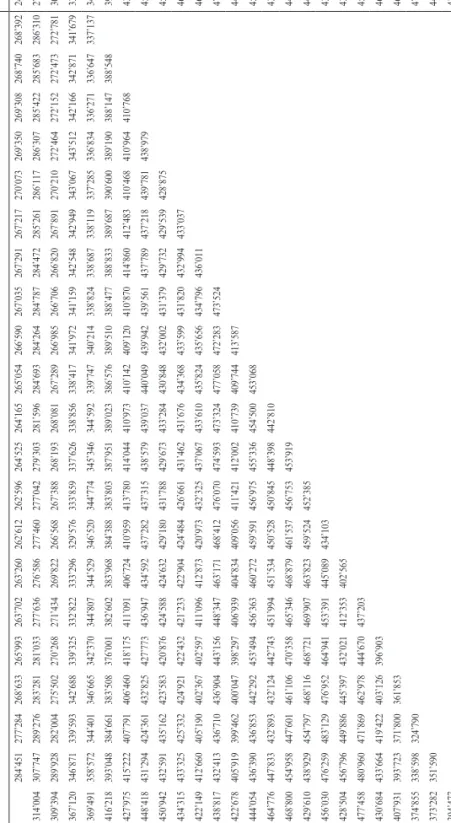
6.1. Industrial Property Insurance

Let us fi rst consider data from industrial property, which is given in Table 5 in Appendix B. We apply the estimators suggested in Section 5 and refer to them