HAL Id: lirmm-02413025
https://hal-lirmm.ccsd.cnrs.fr/lirmm-02413025
Preprint submitted on 16 Dec 2019
HAL is a multi-disciplinary open access
archive for the deposit and dissemination of
sci-entific research documents, whether they are
pub-lished or not. The documents may come from
teaching and research institutions in France or
abroad, or from public or private research centers.
L’archive ouverte pluridisciplinaire HAL, est
destinée au dépôt et à la diffusion de documents
scientifiques de niveau recherche, publiés ou non,
émanant des établissements d’enseignement et de
recherche français ou étrangers, des laboratoires
publics ou privés.
Cutting an alignment with Ockham’s razor
Mark Jones, Philippe Gambette, Leo van Iersel, Remie Janssen, Steven Kelk,
Fabio Pardi, Celine Scornavacca
To cite this version:
Mark Jones, Philippe Gambette, Leo van Iersel, Remie Janssen, Steven Kelk, et al.. Cutting an
alignment with Ockham’s razor. 2019. �lirmm-02413025�
arXiv:1910.11041v1 [q-bio.PE] 24 Oct 2019
(will be inserted by the editor)
Cutting an alignment with Ockham’s razor
Mark Jones · Philippe Gambette · Leo van Iersel · Remie Janssen · Steven Kelk · Fabio Pardi · Celine Scornavacca
Received: date / Accepted: date
Abstract In this article, we investigate different parsimony-based approaches towards finding re-combination breakpoints in a multiple sequence alignment. This rere-combination detection task is crucial in order to avoid errors in evolutionary analyses caused by mixing together portions of se-quences which had a different evolution history. Following an overview of the field of recombination detection, we formulate four computational problems for this task with different objective func-tions. The four problems aim to minimize (1) the total homoplasy of all blocks (2) the maximum homoplasy per block (3) the total homoplasy ratio of all blocks and (4) the maximum homoplasy ratio per block. We describe algorithms for each of these problems, which are fixed-parameter tractable (FPT) when the characters are binary. We have implemented and tested the algorithms on simulated data, showing that minimizing the total homoplasy gives, in most cases, the most accurate results. Our implementation and experimental data have been made publicly available. Finally, we also consider the problem of combining blocks into non-contiguous blocks consisting of at most p contiguous parts. Fixing the homoplasy h of each block to 0, we show that this problem is NP-hard when p ≥ 3, but polynomial-time solvable for p = 2. Furthermore, the problem is FPT with parameter h for binary characters when p = 2. A number of interesting problems remain open.
Keywords Recombination breakpoints, homoplasy, parsimony, block partitioning, exact algorithms, experiments, fixed parameter tractability.
Mathematics Subject Classification 68Q25 92D15 92D20
Research funded in part by the Netherlands Organization for Scientific Research (NWO), including Vidi grant 639.072.602 and Gravitation grant NETWORKS-024.002.003, and partly by the 4TU Applied Mathematics Institute. Mark Jones
Centrum Wiskunde & Informatica (CWI), P.O. Box 94079, 1090 GB Amsterdam, Netherlands. E-mail: [email protected]
Philippe Gambette
Laboratoire d’Informatique Gaspard-Monge (LIGM), Université Paris-Est, CNRS, ENPC, ESIEE Paris, UPEM, F-77454, Marne-la-Vallée, France. Email: [email protected]
Leo van Iersel and Remie Janssen
Delft Institute of Applied Mathematics, Delft University of Technology, Van Mourik Broekmanweg 6, 2628 XE Delft, The Netherlands. E-mail: {L.J.J.vanIersel, R.Janssen-2}@tudelft.nl
Steven Kelk
Department of Data Science and Knowledge Engineering (DKE), Maastricht University, P.O. Box 616, 6200 MD Maastricht, Netherlands. E-mail: [email protected]
Fabio Pardi
LIRMM, Université de Montpellier, CNRS, Montpellier, France. E-mail: [email protected] Celine Scornavacca
Institut des Sciences de l’Evolution, Université de Montpellier, CNRS, IRD, EPHE, 34095 Montpellier Cedex 5, France. E-mail: [email protected]
1 Introduction
When a multiple alignment contains sequences whose ancestors have undergone recombination, the evolutionary histories of different parts of the alignment are represented by different phylo-genetic trees. In this case, using standard evolutionary analysis tools that assume a single phy-logenetic tree for the entire alignment can introduce important biases for several inference tasks. For example it has been shown that in the presence of recombination, positive selection pres-sures (Anisimova et al. 2003; Kosakovsky Pond et al. 2008;Arenas and Posada 2010a), as well as rate variation among sites and lineages tends to be overestimated (Schierup and Hein 2000a,b). Recombination can also severely affect the inference of genetic distances (Schierup and Hein 2000a;
Lemey and Posada 2009), of ancestral sequences (Arenas and Posada 2010b), of demographic his-tory (Schierup and Hein 2000a), and of course of the phylogeny itself, which may bear little resem-blance to the true reticulate history of the sequences (Posada and Crandall 2002).
An often viable solution to these problems is to partition the input alignment into recombination-free blocks, which can then be analysed with standard methods using a single phylogenetic tree per block (see, e.g.,Scheffler et al. 2006, for its application to the detection of positive selection in viruses). Inferring “locus trees” for a large number of recombination-free blocks has also become very popular in the context of species tree inference under the multi-species coalescent model (see
Xu and Yang 2016, for a recent review), where metiotic recombination is assumed to have happened between—but not within—blocks.
For these reasons, a recurring preliminary step in evolutionary bioinformatics is to infer the putative locations within an alignment where recombination has occurred, that is, the recombination break-points, with the goal of partitioning the alignment into blocks for further downstream analyses. In this paper, we closely examine a number of formulations of the problem of alignment partitioning in the presence of recombination, and algorithms that allow to efficiently solve them. Many increas-ingly sophisticated methods have been proposed for this or similar tasks (Salminen and Martin 2009; Martin et al. 2011). Below, we present an overview of the main ideas behind these meth-ods.
Phylogenetic incompatibilities between sites in an alignment can either be due to recurrent sub-stitutions—that is, the same or the inverse substitution having arisen on different branches in the tree—or to recombination having occurred between those sites (see box 15.1 inLemey and Posada 2009). Distinguishing between these two phenomena—recurrent substitution and recombination— is strongly influenced by the prior belief about their relative frequencies. For example, if recurrent substitutions are assumed to be impossible (the infinite sites model ), every pair of incompatible sites must be separated by a recombination breakpoint, an observation that led to one of the earliest methods for breakpoints estimation (Hudson and Kaplan 1985). On the other hand, classi-cal phylogenetic inference assumes no recombination, and all incompatibilities between characters are explained by recurrent substitution. When both recombination and recurrent substitution are possible, an observation that underlies virtually all the methodology for recombination detection (and the present work is no exception) is that recombination leads to the spatial clustering along the alignment of compatible or nearly-compatible sites. In other words, in the presence of recom-bination, sites carrying similar phylogenetic signals tend to be closer than expected by chance alone.
The literature about recombination detection is very rich. A review from 2011 reported that there were already about 90 tools available at the time (see Table S1 inMartin et al. 2011). In prac-tice, however, these were conceived with many different tasks and goals in mind (e.g., detecting evidence of recombination, estimating breakpoints, identifying the parental sequences of the re-combinants, etc.). Although it is beyond the scope of this article to provide a complete overview, there are a number of recurring ideas that are easy to describe. The methods allowing the identifi-cation of breakpoints in a multiple alignment can be roughly categorized in 3 groups (Martin et al. 2011).
Similarity- or distance-based methods constitute the conceptually simplest approach. They inspect the variation along the alignment of the (dis-)similarity between sequences, measured in terms of percent identity or of evolutionary distance (estimated via standard substitution models). Changes along the alignment in the relative similarities among sequences are interpreted as evidence of
recombination. Examples of this approach are Rip (Siepel et al. 1995), PhilPro (Weiller 1998), SimPlot(Lole et al. 1999), Rat (Etherington et al. 2004) and T-Recs (Tsimpidis et al. 2017). A problem with these methods is that the relation between pairwise similarities and phylogenetic relatedness is not straightforward, for example because of rate variation among lineages or selec-tion pressures, meaning that a change in relative similarity does not always indicate phylogenetic incongruence or recombination (Lemey and Posada 2009).
Substitution distribution methods focus on a small subset of sequences (e.g., a triple) and, for each such subset in the alignment, they test whether some site patterns (e.g., those with the form xxy, xyx and xyy) occur in clustered locations along the alignment. Recombination breakpoints are identified with those positions where, as we move along the alignment, a change in the relative frequencies of these patterns is detected. These methods are often, but not exclusively, based on the use of a sliding window. Examples of this approach are GeneConv (Sawyer 1989;Padidam et al. 1999), MaxChi (Smith 1992), Chimaera (Posada and Crandall 2001; Martin et al. 2010), Sis-can(Gibbs et al. 2000), 3-Seq (Boni et al. 2007;Lam et al. 2017), Rapr (Song et al. 2018). The necessity to analyse only a subset at a time, instead of all sequences simultaneously, may be prob-lematic when the alignment contains many sequences. This is not just for computational reasons (e.g., the number of triples grows cubically in the number of sequences) and statistical reasons (correcting for the rapidly increasing multiple tests may lower the power to detect recombina-tion (Martin et al. 2017)). Another important issue is that the situation where the alignment only contains sequences that are direct recombinants of other sequences within the alignment is in fact the exception rather than the rule. If an alignment contains several descendants of the same re-combinant, or a parental sequence of a recombinant is the ancestor of several sequences in the alignment, then the same recombination event should be detected in several partially overlapping subsets. Being able to recognize when two subsets have detected the same event is a difficult and open question (Song et al. 2018).
Phylogenetic-based methods seek to detect when different contiguous blocks in the alignment support different phylogenetic trees. A seminal paper in this context is due to J. Hein (Hein 1993). That paper introduced an optimization problem whose goal is to determine a sequence of breakpoints in the alignment and a sequence of phylogenetic trees for each of the blocks de-limited by the breakpoints, so as to minimize a linear combination of the parsimony scores of the trees and of the cost of breakpoints. Each breakpoint has a cost that expresses the mini-mum number of recombination events that are necessary to “switch” between the two trees that it separates. Solving this problem exactly is impractical for several reasons (see the formal defini-tion and discussion in Sec. 9.8.1 of Huson et al. 2010), so a heuristic named RecPars was pro-posed (Hein 1993;Huson et al. 2010). Subsequent methods relied on distance-based phylogenetics (e.g., BootScan (Salminen et al. 1995), Topal (McGuire et al. 1997)), maximum-likelihood
tech-niques (e.g., Plato (Grassly and Holmes 1997), Lard (Holmes et al. 1999), Gard (Kosakovsky Pond et al. 2006a,b)), while more recent methods use hidden Markov models whose hidden states correspond
to phylogenetic trees, and where the observations are the columns of the alignment. These models, sometimes referred to as phylo-HMMs, can be used to infer probable partitions of the input align-ment into recombination-free blocks and are at the core of tools such as Barce (Husmeier and McGuire 2003), DualBrothers (Minin et al. 2005), StHmm (Webb et al. 2008) and many others (Hobolth et al. 2007; Bloomquist et al. 2008; de Oliveira Martins et al. 2008; Dutheil et al. 2009; Boussau et al. 2009). Although phylogenetic-based methods are very appealing as they directly look for phyloge-netic incongruence—instead of relying on indirect evidence from pairwise similarities or site pat-tern frequencies—they are usually much more computationally demanding than similarity-based or substitution distribution methods. In practice, sophisticated methods such as those based on phylo-HMMs are only applicable to a small number of sequences (e.g., 4 forHusmeier and McGuire 2003), unless the space of tree topologies that can be assigned to the blocks is heavily restricted (Minin et al. 2005; Webb et al. 2008). For this reason, some authors have proposed the use of parsimony cri-teria (Hein 1993; Maydt and Lengauer 2006;Ruths and Nakhleh 2006;Ané 2011), well-known to lead to faster computations at the cost of some loss in accuracy. We note in particular the Mdl approach byAné (2011), which seeks to solve an optimization problem that is a simplification of that byHein(1993) mentioned above, in that all breakpoints receive the same penalty.
The work we present here falls naturally in this context of phylogenetic- and parsimony-based methods for recombination-aware alignment partitioning. Our goal is not to present a new software tool for this task—although we do provide implementations of some novel algorithms—but to
investigate a number of natural formulations of the problem, and provide exact algorithms to solve them. We also investigate the relative strengths of the alternative formulations. Our optimization problems are defined in terms of the homoplasy within each block (informally, the amount of recurrent substitution that is needed to explain the sequences in that block), although equivalent formulations could be expressed in terms of parsimony scores. This choice is motivated by the observation that deciding whether a block has a level of homoplasy below a (small) constant is polynomially solvable (Fernández-Baca and Lagergren 2003; Sridhar et al. 2007).
Another key choice we made is related to the well-known observation that the number of blocks inferred by many methods for alignment partitioning is sensitive to parameters such as the size of a sliding window, or the cost/penalty of breakpoints or recombinations, relative to that of sub-stitutions, for parsimony-based methods such as RecPars and Mdl (Hein 1993; Ané 2011). To a lesser extent, this also holds for HMM-based statistical approaches, which rely on the use of priors on breakpoint frequency (Husmeier and McGuire 2003) or on the total number of break-points (Minin et al. 2005). In our problem formulations, instead of introducing a parameter that indirectly influences the number of blocks inferred, we chose to directly constrain the maximum number of blocks in the partition. We believe this has the merit of making more explicit the dependency of block partitioning on user-defined parameters.
Overview of the article. We start by introducing necessary preliminaries in Section2, and then move on to defining four different parsimony-based models for detecting recombination breakpoints in Section 2.1. Some of these models aim to minimize the maximum homoplasy in a block—or the relative frequency of homoplasy in a block—while others take an aggregate perspective, consider-ing all blocks together. Although these models constitute fairly natural optimization criteria for parsimony-based models, one of our primary contributions is that, for all models, explicit pseu-docode, rigorous proofs of correctness and detailed running time analyses are given: these are provided in Section 3. Several of the algorithms are Fixed Parameter Tractable (FPT) for bi-nary characters, meaning—in essence—that certain natural parameters of the problems have an independent, and thus limited, contribution to the overall running time (We refer the reader to
Flum and Grohe 2006; Downey and Fellows 2012, for more background on FPT algorithms). In Section4we describe algorithms that attempt to merge blocks, from a pre-computed block parti-tion, such that parsimony-motivated criteria are optimized (these models are formally defined in Section2.2). In Section 5 we describe our publicly-available software package CutAl, which im-plements the four algorithms described in Section3. We have performed a number of experiments on simulated data testing the ability of the four algorithms to recover the locations of breakpoints; in particular, we look at the influence of the number and length of blocks, the number of taxa and the branch lengths (of the phylogenies used to experimentally generate alignments) on the over-all performance of the algorithms. This data has also been made publicly available. Our analysis suggests that, of our four algorithms, aggregate minimization of the total amount of homoplasy seems most effective, and is highly accurate under many variations of experimental parameters. In Section6we present our overall conclusions and propose a number of interesting directions for future work.
2 Preliminaries
Let S be a set of character states. Throughout the paper, we assume that the cardinality s of S is a constant. An alignment A is an n × m matrix with elements from S. Denote by Aj the j-th column
of A and denote by Ai,j the element in the i-th row and j-th column of A, for any 1 ≤ i ≤ n and
1 ≤ j ≤ m. We also refer to the columns of an alignment as characters.
A block A[i − j] in A is the alignment formed by the columns Ai, . . . , Aj, for some 1 ≤ i ≤ j ≤ m.
When A is clear from context we will write [i − j] as shorthand for A[i − j]. When the indices i and j are not important, we often write B to denote a block. Note that blocks are always composed of contiguous columns. The number of columns in a block B is denoted |B|. A block partitioning of A is a partition B = B1, . . . Bb of the columns of A, such that each Bh is a block.
The null score s0(A) of an alignment A is Pmj=1s0(Aj), with s0(Aj) the number of different
A phylogenetic tree on X is an unrooted tree with no degree-2 vertices and leaf set X. An h-near perfect phylogeny for an alignment A is a phylogenetic tree T = (V, E) on {x1, . . . , xn} with a
mapping τ : V → Smsuch that τ (x
i) = Ai and
X
{u,v}∈E
dh(τ (u), τ (v)) ≤ s0(A) + h
with dh(s1, s2) the Hamming distance of s1 and s2 (the number of positions where they differ).
The parsimony score P S(T, A) can now be defined as the minimum value of s0(A) + h such that T
is an h-near perfect phylogeny for A. A 0-near perfect phylogeny is a perfect phylogeny, which has parsimony score s0(A).
An alignment A is said to have homoplasy score h if h is the minimum integer for which there exists an h-near perfect phylogeny for A. The total homoplasy of a block partitioning is the sum of the homoplasies of its blocks. Observe that the total homoplasy of a block partition of an alignment is at most the homoplasy of the alignment. Denote by h(B) the homoplasy of a block B. Denote by r(B) =h(B)|B| the homoplasy ratio of B.
We note some established results concerning the calculation of homoplasy scores. In particular, we note that calculating the homoplasy score of an alignment is fixed-parameter tractable for binary characters:
Theorem 1 (Sridhar et al. 2007) Given an n×m alignment A with elements from S with |S| = 2, it can be decided in O(21h+ 8hnm2) time whether A has an h-near perfect phylogeny.
Theorem 2 (Fernández-Baca and Lagergren 2003) Given an n × m alignment A with elements from S with |S| = s, it can be decided in O(nmO(h)2O(h2
s2
)) time whether A has an h-near perfect
phylogeny.
We also recall the well-known four-gamete test (Buneman 1971), which characterizes alignments for which there exists a perfect phylogeny when |S| = 2.
Theorem 3 (Four-gamete test) (Buneman 1971) Let A be an alignment on S where S = {0, 1}. Call two characters j, k of A incompatible if there exist rows i1, i2, i3, i4 such that
Ai1,j= 1 = 1 = Ai1,k
Ai2,j= 1 6= 0 = Ai2,k
Ai3,j= 0 6= 1 = Ai2,k
Ai4,j= 0 = 0 = Ai4,k.
Then A has homoplasy score 0 if and only if no two characters of A are incompatible.
A column Aj is called an uninformative site if some character state s ∈ S appears n − s0(Aj)
times in Aj, and every other character state appears at most once. Otherwise, Ajis an informative
site. Observe that a column Aj is an uninformative site if and only if every phylogenetic tree on
{x1, . . . , xn} is a perfect phylogeny for Aj. From a parsimony perspective, uninformative sites
pro-vide no meaningful information, and we will therefore ignore them when considering the accuracy of block partitions (see Section5). For a given block B in A that contains at least one informative site, let B′be the minimal contiguous block in B that contains all the informative sites of B. Then
we call B′ the informative restriction of B. Note that B′ can still contain uninformative sites,
but the first and last columns in B′ are guaranteed to be informative. A block B is said to be
completely uninformative if every column in B is an uninformative site. Given a block partition B of A, the informative restriction of B is derived from B by deleting all completely uninformative blocks, and replacing each remaining block with its informative restriction.
2.1 Partitioning into contiguous blocks
We consider a number of block partitioning problems in which the aim is to partition an alignment into a small number of blocks with homoplasy as small as possible.
Total Homoplasy Score
Given: an alignment A and integer b.
Find: a block partitioning of A into b′≤b blocks B
1, . . . , Bb′, such that P
b′
i=1h(Bi) is
mini-mized.
Max Homoplasy Ratio
Given: an alignment A and integer b.
Find: a block partitioning of A into b′≤b blocks B1, . . . , Bb′, such that maxb ′
i=1r(Bi) is
mini-mized.
Max Homoplasy Score
Given: an alignment A and integer b.
Find: a block partitioning of A into b′≤b blocks B
1, . . . , Bb′, such that maxb ′
i=1h(Bi) is
mini-mized.
Total Homoplasy Ratio
Given: an alignment A and integer b.
Find: a block partitioning of A into b′≤b blocks B1, . . . , Bb′, such that
Pb′
i=1r(Bi) is
mini-mized.
Note that the variant of these four problems when the blocks in the output are not required to be contiguous is NP-complete, as it was proved byLinz et al.(2013) that the restricted case where the total homoplasy is 0 and the number of blocks is fixed to an integer b ≥ 3 (called b-Character-Compatibility) is NP-complete.
2.2 Combining blocks to non-contiguous blocks
A multiblock for an alignment A is an alignment formed by some subset of columns in A. Thus, the difference between a block and multiblock is that a multiblock is not necessarily contiguous. We say a multiblock is a p-multiblock if it can be partitioned into at most p contiguous parts—i.e., it is the union of at most p blocks. A non-contiguous block partitioning of an alignment A is a partitioning of the columns of A into mulitblocks. The total homoplasy of a non-contiguous block partitioning is defined similarly as for block partitionings. The next problem studied in this paper aims at merging blocks with small total homoplasy to a small number of non-contiguous blocks. It is formally defined as follows.
Block Combining
Given: an alignment A, a block partitioning B of A with total homoplasy h and an integer c. Decide: does there exist a non-contiguous block partitioning with total homoplasy h that consists of at most c non-contiguous blocks, each of which is a union of blocks from B?
Since allowing blocks to be completely atomized into many small contiguous parts seems to be too flexible, we also consider a variant where we only allow a partition into p-multiblocks.
We say that two blocks Bj and Bk are mergeable if their union Bj ∪ Bk has homoplasy equal to
the homoplasy of Bj plus the homoplasy of Bk. In the following problem, we assume that input
blocks Bjand Bj+1are not mergeable for any j. This is a reasonable assumption in cases where the
input block partition is derived from a block partitioning algorithm. It holds, for example, when the blocks are those generated by Algorithm3, and it also holds for solutions to Total Homoplasy Scoreprovided the value of b is chosen to be as small as possible without increasing h.
Block Combining top-Multiblocks
Given: an alignment A, a block partitioning B of A with total homoplasy h such that Bj and
Bj+1 are not mergeable for any j, and integer c.
Decide: does there exist a non-contiguous block partitioning with total homoplasy h that consists at most c p-multiblocks, each of which is a union of blocks from B?
3 Block partitioning algorithms 3.1 Minimizing total homoplasy
In this section, we describe an approach that can be used to solve the Total Homoplasy Score problem. The key observation is that, given a suitable method to calculate the homoplasy score of each possible block in A, an optimal block partitioning can be found using standard dynamic programming techniques. Algorithm1 describes this dynamic programming technique, under the assumption that a value φ(B) has been calculated for each possible block B. For the purposes of solving Total Homoplasy Score, we let φ(B) be the homoplasy score of block B. How-ever, by changing the function φ we can also use Algorithm 1 to solve other block partitioning problems.
In particular, for the implementation described in Section 5, we will not use exact homoplasy scores for φ, but instead use the values returned by the heuristic parsimony solver Parsimonator (https://sco.h-its.org/exelixis/web/software/parsimonator/index.html).
We begin by proving the correctness of Algorithm1with respect to an arbitrary function φ.
Lemma 1 Given an alignment A with columns A1, . . . , Am, an integer b, and a value φ(B) for each
block B in A, Algorithm1returns the minimum value h for which there exists a block partitioning B1, . . . , Bb′ of A into b′ ≤ b blocks such that
Pb′
i=1φ(Bi) = h, or ∞ if no such block partitioning
exists.
Proof For each triplet of integers (i, j, b′) such that 1 ≤ i ≤ j ≤ m and 1 ≤ b′ ≤ b, Algorithm 1
calculates a value hpart(i, j, b′). We first claim that for each choice of (i, j, b′), hpart(i, j, b′) is
equal to the minimum h for which there exists a block partitioning B1, . . . , Bb′ of A[1 − j] with
Pb′
i′=1φ(Bi′) = h, such that Bb′ = A[i − j], i.e., the last block consists of columns Ai to Aj, and
that hpart(i, j, b′) = ∞ if no such block partitioning exists.
We prove this claim by induction on j. We start with the base case, j = 1. In this case, the only possible partitioning on A[1 − j] is the one consisting of the single block B1 = [1 − 1]. Thus
hpart(i, j, b′) should be equal to φ([1 − j]) if i = b′= 1, and ∞ otherwise. It can be seen that this
is the value calculated by Algorithm1, and thus the claim is correct for j = 1.
Now suppose that j > 1. If i = 1, then the only possible block partitioning is the one consisting of the single block B1= [1 − j]. Thus hpart(i, j, b′) should be equal to φ([1 − j]) if i = b′ = 1, and
∞ otherwise. Again this is the value calculated by Algorithm1. If i > 1, then we have that an optimal block partitioning consists of a b′− 1-block partitioning for A[1 − (i − 1)] together with the block [i − j]. Moreover, the last block in the block partitioning of A[1 − (i − 1)] must be [i′− (i − 1)]
for some i′≤ i − 1. Thus in the case j > 1, i > 1, the total valuePb′
i=1φ(Bi) for an optimal block
partitioning B1, . . . , Bb′ of [1 − j] is equal to hpart(i′, i − 1, b′− 1) + φ([i − j]), for the choice of i′
that minimizes this value. As this is exactly what the algorithm calculates, the claim is correct. This completes the inductive proof.
It remains to observe that any block partitioning of A into at most b blocks must have exactly b′
blocks for some 1 ≤ b′ ≤ b, and the last block must be A[i − m] for some 1 ≤ i ≤ m. It follows
that the value of an optimal block partitioning can be found by taking the minimum value of hpart(i, m, b′) for all choices of i and b′. ⊓⊔
The following Lemma is clear from the structure of Algorithm1and is stated without proof.
Lemma 2 Given an alignment A with columns A1, . . . , Am, an integer b, and a value φ(B) for
each block B in A, Algorithm1has running time O(bm3).
Although we do not give a full proof here, we observe that Algorithm1can easily be converted into an algorithm that returns a block partitioning B1, . . . , Bb′ of A into b′≤ b blocks that minimizes
Pb′
by finding the value i for which hpart(i, j, b′) is minimized, recursively finding an optimal block
partitioning for A[1 − (i − 1)] with b′− 1 blocks (if i > 1), and combining this block partitioning
with the block Bb′ = A[i − j]. We therefore have the following lemma.
Lemma 3 Let φ be a function on blocks of A such that the value of φ(B) can be calculated in f (n, m) time for any block B, and let b be an integer. Then in f (n, m)m2+ O(bm3) time, we can calculate a block partitioning B1, . . . , Bb′ of A into b′≤ b blocks such thatP
b′
i=1φ(Bi) is minimized.
The m2factor comes from the need to calculate φ(B) for each of the O(m2) blocks B in A.
Using Theorems1and2 we can now prove the following theorem.
Theorem 4 For binary characters, the Total Homoplasy Score problem can be solved in time O(h21h+ 8hhnm4), where h is is the maximum homoplasy of a block in the block partitioning, and
is thus fixed-parameter tractable with respect to h. For s-state characters, the problem can be solved in time O(hnmO(h)2O(h2
s2
)).
Proof Recall that by Theorem1, for binary characters it can be decided in O(21h+8hnm2) whether
an alignment has an h-near perfect phylogeny (Sridhar et al. 2007). It follows that given an integer h, the homoplasy score of a block can be found in O(h21h+ 8hhnm2) time if this score is at most
h. Similarly by Theorem2, for s-state characters, the homoplasy score of a block can be found in O(hnmO(h)2O(h2
s2
)) time if this score is at most h (Fernández-Baca and Lagergren 2003).
So now, given an integer h let φ be the function on blocks in A such that φ(B) is equal to the homoplasy score of block B if this is at most h, and φ(B) = ∞ otherwise. It remains to apply Lemma3 using this function, with f (n, m) = O(h21h+ 8hhnm2) for binary characters and
f (n, m) = O(hnmO(h)2O(h2
s2
)) for s-state characters. For binary characters, this gives a running
time of O(h21h+ 8hhnm2)m2+ O(bm3) = O(h21h+ 8hhnm4) (as we may assume b ≤ m), and for
s-state characters a running time of O(hnmO(h)2O(h2
s2))m2+ O(bm3) = O(hnmO(h)2O(h2
s2)) (as
O(mO(h)) · m2+ O(bm3) = O(mO(h)+2+4) = O(mO(h)). ⊓⊔
We also observe that by letting φ(B) be the homoplasy ratio of a block B, Algorithm1 can be used to solve Total Homoplasy Ratio.
Data:Alignment A with columns A1, . . . , Am, integer b, a value φ(B) for each block B in A (for instance, φ(B) is
the homoplasy score of B).
Result:Minimum value h for which there exists a block partitioning B1, . . . , Bb′ of A into b′≤ b blocks such that
Pb′
i=1φ(Bi) = h, or ∞ if no such block partitioning exists.
for j = 1, . . . , m do hpart(1, j, 1) := φ([1 − j]); for i = 2, . . . , j do hpart(i, j, 1) := ∞; end for b′= 2, . . . , b do hpart(1, j, b′) = ∞; for i = 2, . . . , j − 1 do
hpart(i, j, b′) := min1≤i′≤i−1hpart(i′, i − 1, b′− 1) + φ([i − j]);
end end end
return minb′≤b,i≤mhpart(i, m, b′)
Algorithm 1: Algorithm ToHoPar(A, b).
3.2 Minimizing homoplasy ratio per block
In this section, we describe an approach that can be used to solve the Max Homoplasy Ratio problem. Similarly to Total Homoplasy Score, the key observation is that after calculating
the homoplasy score (and thus the homoplasy ratio) of each possible block in A, an optimal block partitioning can be found using standard dynamic programming techniques. Algorithm2describes this dynamic programming technique, under the assumption that a value φ(B) has been calculated for each possible block B. For the purposes of solving Max Homoplasy Ratio, we let φ(B) be the homoplasy score of block B.
Data:Alignment A with columns A1, . . . , Am, integer b, a value φ(B) for each block B in A (for instance, φ(B) is
the homoplasy ratio of B).
Result:Minimum value r for which there exists a block partitioning B1, . . . , Bb′ of A into b′≤ b blocks such that
maxb′
i=1φ(Bi) = r, or ∞ if no such block partitioning exists.
for j = 1, . . . , m do rpart(1, j, 1) := φ([1 − j]); for i = 2, . . . , j do rpart(i, j, 1) := ∞; end for b′= 2, . . . , b do rpart(1, j, b′) = ∞; for i = 2, . . . , j − 1 do
rpart(i, j, b′) := max(φ([i − j]), min1≤i′≤i−1rpart(i′, i − 1, b′− 1));
end end end
return minb′≤b,i≤mrpart(i, m, b′)
Algorithm 2: Algorithm HoRaPar(A, b).
Lemma 4 Given an alignment A with columns A1, . . . , Am, an integer b, and a value φ(B) for each
block B in A, Algorithm2returns the minimum value r for which there exists a block partitioning B1, . . . , Bb′ of A into b′≤ b blocks such that maxb
′
i=1φ(Bi) = r, or ∞ if no such block partitioning
exists.
Proof Observe that Algorithm2 is identical to Algorithm 1, except for line 9 which handles con-struction of rpart(i, j, b′) in the case where b′ > 1 and j > i > 1. Consequently, the proof of this
lemma is identical to that of Lemma1, except for the case b′ > 1 and j > i > 1, and we omit the
other cases.
As with Lemma 1, we prove by induction on j that rpart(i, j, b′) is equal to the minimum r for
which there exists a block partitioning B1, . . . , Bb′ of A[1 − j] with maxb ′
i′=1φ(Bi′) = r, such that
Bb′ = A[i − j], and that rpart(i, j, b′) = ∞ if no such block partitioning exists. For the case b′> 1
and j > i > 1, we have that an optimal block partitioning consists of a b′− 1-block partitioning
for A[1 − (i − 1)] together with the block [i − j]. Moreover, the last block in the block partitioning of A[1 − (i − 1)] must be [i′− (i − 1)] for some i′ ≤ i − 1. Thus the value maxb′
i=1φ(Bi) for an
optimal block partitioning B1, . . . , Bb′ of [1 − j] is equal to the maximum of rpart(i′, i − 1, b′− 1)
and φ([i − j]), for the choice of i′ that minimizes this value. As this is exactly what the algorithm
calculates, the claim is correct, and we have completed the proof for this case. ⊓⊔
The following Lemma is clear from the structure of Algorithm2and is stated without proof. Lemma 5 Given an alignment A with columns A1, . . . , Am, an integer b, and a value φ(B) for
each block B in A, Algorithm2has running time O(bm3).
As with Algorithm1, we observe that Algorithm2can be made to return a block partitioning using standard backtracking techniques, and that using existing homoplasy algorithms, a certain param-eterization of Max Homoplasy Ratio for binary characters is fixed-parameter tractable. Theorem 5 For binary characters, the Max Homoplasy Ratio problem can be solved in time O(h21h+ 8hhnm4), where h is is the maximum homoplasy of a block in the block partitioning, and
is thus fixed-parameter tractable with respect to h. For s-state characters, the problem can be solved in time O(hnmO(h)2O(h2
s2
)).
We also observe that by letting φ(B) be the homoplasy score of a block B, Algorithm1 can be used to solve Max Homoplasy Score.
3.3 Minimizing number of blocks
In this section, we consider a variation of the Max Homoplasy Score problem, described be-low.
Fewest Parsimonious Blocks Given: an alignment A and integer h.
Find: a block partitioning B1, . . . , Bb, of A into a minimum number of blocks such that each block
Bk admits an h-near perfect phylogeny.
Algorithm3 solves the Fewest Parsimonious Blocks problem.
Data:Alignment A with columns A1, . . . , Amand an integer h.
Result:Block partitioning B1, . . . , Bbof A into a minimum number of blocks, such that each block Bkadmits an
h-near perfect phylogeny. b := 1;
j := 1;
for i = 2, . . . , m do
if A[j − i] does not admit an h-near perfect phylogeny then Bb:= A[j − (i − 1)]; b := b + 1; j := i end end Bb:= A[j − m]; return B1, . . . , Bb
Algorithm 3: Algorithm FewParBlo(A, h)
Theorem 6 Algorithm3solves the Fewest Parsimonious Blocks problem.
Proof Let B1, . . . , Bb be a block partitioning produced by Algorithm 3, and let F1, . . . , Fc be a
block partitioning into a minimum number of blocks such that the index of the first column where B1, . . . , Bb and F1, . . . , Fc differ (i.e., the minimum i such that columnn Ai appears in blocks Bk
and Fk′ for some k 6= k′) is as large as possible. Consider the smallest k for which Fk 6= Bk.
It is not possible that Fk has more columns than Bk since otherwise the algorithm would have
extended Bk with another column. Hence, Fk has fewer columns than Bk. However, then we can
add a column to Fk and obtain a solution with the same number of blocks as F1, . . . , Fc where the
first columns where it differs from B1, . . . , Bb is one larger. This contradicts the assumption that
the first column where B1, . . . , Bb and F1, . . . , Fc differ is as large as possible. Hence, we conclude
that B1, . . . , Bb is identical to F1, . . . , Fc and therefore optimal. ⊓⊔
The running time of Algorithm 3 is m times the running time of the h-near perfect phylogeny algorithm, hence O(21hm + 8hnm3) for binary characters and O(nmO(h)2O(h2
s2
)) for general
s-state characters. Consequently, the Fewest Parsimonious Blocks problem is fixed-parameter tractable for binary characters.
Corollary 1 Fewest Parsimonious Blocks is fixed-parameter tractable when the parameter is h for binary characters.
If the number of blocks b is known to be small (b ≤ m/ log m), the following algorithm may also be useful. It uses binary search to find the location of the recombination site between two blocks.
The correctness of this algorithm follows from a similar argument as for the previous algorithm: this algorithm uses binary search instead of linear search to find the longest possible block, using l and u2as lower and upper bounds on the last column of that block. The only extra observation needed is
the following. If A[i−j] admits an h-near perfect phylogeny, then so does A[i−(j−1)]; and, similarly, if A[i − j] does not admit an h-near perfect phylogeny, then neither does A[i − (j + 1)].
Note that the running time of the part within the while loop is dominated by the function checking whether an h-near perfect phylogeny exists. As this while loop performs a binary search on a list
Data:Alignment A with columns A1, . . . , Amand an integer h.
Result:Block partitioning B1, . . . , Bkof A into a minimum number of blocks, such that each block Biadmits an
h-near perfect phylogeny. end_previous_block := 0; while end_previous_block < m do l =end_previous_block + 1; u2= m; while l < u2do u1= ⌈(l + u2)/2⌉;
if A[(end_previous_block + 1) − u1]admits an h-near perfect phylogeny then
l := u1; else u2:= u1− 1; end end Bb:= A[(end_previous_block + 1) − u2]; b := b + 1; end_previous_block := u2; end return null;
Algorithm 4: Algorithm FewParBlo2(A, h, b)
of length m − l, its contents are executed log2(m − l) < log2(m) times. Finally, this while loop
is contained in a for loop which runs b times at most. Therefore the running time is bounded by b log2(m) times the running time of the h-near perfect phylogeny algorithm, which theoretically
gives a factor m/(b log2m) improvement over the previous algorithm. An important note here is
that actual running time may also depend on implementation of the h-near perfect phylogeny algorithm. If the worst case for this algorithm is only attained in NO cases, the improvement of the second algorithm may be less than expected as the first algorithm encounters exactly one NO case per block, and the second may encounter more such cases.
4 Combining blocks to non-contiguous blocks
We now consider the Block Combining to p-Multiblocks problem and first show this problem to be NP-complete for p ≥ 3 by reduction from the Bounded Coloring problem: given a graph G, does there exist a coloring of the vertices of G with at most c colors such that each color is used at most p times and adjacent vertices always get different colors? This problem is NP-complete for each fixed p ≥ 3 (Hansen et al. 1993).
Theorem 7 For every integer p ≥ 3, the Block Combining to p-Multiblocks problem is NP-complete for h = 0.
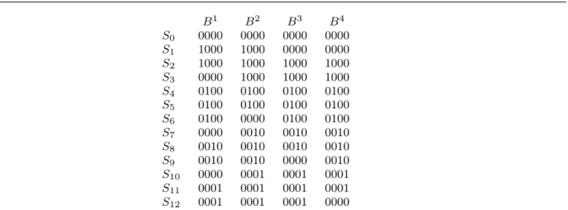
Proof Given an instance of the Bounded Coloring problem, that is an integer p ≥ 3 and a graph G = (V, E) with n = |V |, we build the following blocks Bj of 3n + 1 aligned sequences
S0, S1, . . . , S3n of length n for each vertex vj of G, illustrated in Figure1:
– B0,kj = 0 for all k ∈ {1, . . . , n} (that is, the first row in Bj consists of all 0’s);
– B3j−2,jj = B3j−1,jj = 1 and Bjk,j= 0 for all k in {1, . . . , 3j − 3} ∪ {3j, . . . , n};
– for all i ∈ [1, . . . , n] distinct from j such that vj adjacent with vi, B3i−1,ij = B3i,ij = 1 and
Bk,ij = 0 for all k ∈ {1, . . . , 3i − 2} ∪ {3i + 1, . . . , n};
– for all i ∈ {1, . . . , n} distinct from j such that vj not adjacent with vi, B j
3i−2,i = B
j
3i−1,i =
B3i,ij = 1 and Bjk,i= 0 for all k ∈ {1, . . . , 3i − 3} ∪ {3i + 1, . . . , n}.
Recall from the four-gamete test that an alignment A has homoplasy 0 if and only if no two characters are incompatible, where characters j, k are incompatible if there exist rows i1, i2, i3, i4
B1 B2 B3 B4 S0 0000 0000 0000 0000 S1 1000 1000 0000 0000 S2 1000 1000 1000 1000 S3 0000 1000 1000 1000 S4 0100 0100 0100 0100 S5 0100 0100 0100 0100 S6 0100 0000 0100 0100 S7 0000 0010 0010 0010 S8 0010 0010 0010 0010 S9 0010 0010 0000 0010 S10 0000 0001 0001 0001 S11 0001 0001 0001 0001 S12 0001 0001 0001 0000
Fig. 1 An instance of the Block Combining to p-Multiblocks problem built from an instance G = {{v1, v2,
v3, v4}, {v1v3, v1v4}} of the Bounded Coloring problem with at most p vertices per color.
First note that by construction, the only characters which may be equal to 1 in each block Bj
are the i-th character of the block on sequences S3i−2, S3i−1 and 3i, all other characters are equal
to 0. Therefore, there is at most one character equal to 1 in each line of block Bj, therefore Bj
contains no incompatible characters, so the block Bj has homoplasy 0, therefore we have built a
proper instance of the Block Combining to p-multiblocks problem for h = 0.
Now, suppose that G is a positive instance of the Bounded Coloring problem using at most c colors used at most p times, then there exist c independent sets I1, . . . , Icin G. We claim that the
corresponding p-multiblocks have homoplasy 0.
To prove this claim, let us consider 2 characters c and c′ in two distinct blocks B and B′ in the
same p-multiblock, such that c is the i-th character of block B and c′ is the i′-th character of
block B′. If i 6= i′, the two characters are compatible because the 1s in those two characters do not
appear in the same line. Otherwise, by construction the only 1s may appear in the sequences S3i−2,
S3i−1 and S3i for these 2 characters. The vertices v and v′ corresponding to blocks B and B′ are
not adjacent because they are part of an independent set, therefore by construction the sequences S3i−2, S3i−1 and S3i all contain 1 for one of these two characters, therefore both characters are
compatible. So in all cases each p-multiblock has homoplasy 0.
To prove the reverse, let us assume that it is possible to merge the blocks of the instance of the Block Combining to p-Multiblocks we have built so that each p-multiblock has homoplasy 0. For each p-multiblock P , let us consider two vertices vi and vi′ of G corresponding to two
blocks Bi and Bi′ of P . Suppose by contradiction that vi and vi′ are adjacent. Then we have
Bi 3i−1,i= 1 = Bi ′ 3i−1,i, B3i−2,ii = 1 6= 0 = Bi ′ 3i−2,i, Bi3i,i= 0 6= 1 = Bi ′
3i,i and B0,ii = 0 = Bi
′
0,i. Thus
the i-th character of block Bi and of block Bi′
are incompatible, and therefore the homoplasy cost of the block combination containing Bi and Bi′
is strictly greater than 0; a contradiction. Therefore, no pair of vertices corresponding to the blocks of the block combination are adjacent, thus each set of vertices corresponding to each of the c block combinations is an independent set, so G has a c-coloring.
Thus, we have built an instance of the Block Combining to p-Multibocks problem where a merge into c non-contiguous blocks (each containing at most p contiguous blocks) with total homoplasy 0 for each of these c blocks is possible if and only if there is a c-coloring of G where each color is used at most p times, therefore Block Combining to p-Multiblocks is NP-hard. Given a merge into c non-contiguous blocks, it is easy to check if all the characters of each of these blocks are compatible, and that each non-contiguous block contains at most p contiguous blocks, so Block Combining to p-Multiblocks is NP-complete. ⊓⊔
We now focus on the case p = 2, i.e., the problem Block Combining to 2-Multiblocks. We now argue correctness of the algorithm. Suppose that there exist c′ 2-multiblocks with total
homoplasy h and such that each of the 2-multiblocks is a union of blocks from B. Each 2-multiblock that consists of exactly two contiguous parts corresponds to an edge of G. Let M′ be the set of
all such edges and observe that they form a matching in G. Each 2-multiblock that consists of a single contiguous part corresponds to a vertex of G. Moreover, each vertex of G that is not covered
Data:Alignment A, a block partitioning B of A with total homoplasy h such that Bjand Bj+1are not mergeable
for any j, and integer c.
Result:At most c 2-multiblocks, each of which is a union of blocks from B, such that the total homoplasy of the 2-multiblocks is h (if such a solution exists).
Construct a graph G = (V, E) with a vertex for each block and an edge {Bj, Bk} if Bj and Bkare mergeable;
Find a maximum matching M in G; for each edge {Bj, Bk} ∈ M do
merge Bj and Bkinto a 2-multiblock;
end
for each vertex Bjthat is not covered by M do
make Bja 2-multiblock consisting of a single continuous part;
end
if the number of obtained 2-multiblocks is at most c then return the obtained 2-multiblocks;
else
return null; end
Algorithm 5: Algorithm BloCo2Mul(A, B, h, c)
by M′corresponds to such a 2-multiblock. Hence, c′ = (|V | − 2|M′|) + |M′| = |V | − |M′|. It follows
that we get the smallest possible number c′ of 2-multiblocks by choosing a maximum cardinality
matching M′, which Algorithm5does.
The following theorem follows directly, since it can be checked in polynomial time whether an alignment has homoplasy 0 (Agarwala and Fernandez-Baca 1994;Kannan and Warnow 1997) and for binary states this is fixed-parameter tractable with parameter h (Sridhar et al. 2007).
Theorem 8 Block Combining to p-Multiblocks can be solved in polynomial time for p = 2 and h = 0 and it is fixed-parameter tractable with parameter h for binary characters and p = 2.
We now continue to the general Block Combining to p-Multiblocks problem with p ≥ 2. This problem can be solved by Algorithm6. We say that a collection of blocks B′ ⊆ B is mergeable
if the total homoplasy of B′is equal to the homoplasy of the alignment obtained by combining all
blocks from B′. Note that, in general, it may happen that a set of blocks is not mergeable even if
the blocks in the set are pairwise mergeable.
Data: Alignment A, a block partitioning B of A with total homoplasy h such that Bjand Bj+1are not
mergeable for any j, and integer c.
Result:At most c p-multiblocks, each of which is a union of blocks from B, such that the total homoplasy of the p-multiblocks is h.
Construct a graph G = (V, E) with a vertex for each set B′⊆ B with |B′| ≤ p that is mergeable and an
edge {B′, B′′} if B′∩ B′′6= ∅;
Give each vertex B′a weight equal to |B′| − 1 (i.e., the number of blocks in B′ minus one);
Find a maximum weight independent set I in G; for each input block B ∈ B not in any element of I do
add the vertex {B} to I; end
for each vertex B′∈ I do
Merge the blocks in B′into a p-multiblock;
end
if the number of obtained p-multiblocks is at most c then return the obtained p-multiblocks
else
return null end
Algorithm 6: Algorithm BloCopMul(A, B, h, c)
Correctness of Algorithm 6 follows from the following argument. First we argue that each p-multiblock partitioning of B with total homoplasy h and c p-multiblocks corresponds to an inde-pendent set in G containing all input blocks B ∈ B of weight |B| − c. Then we show that each independent set I of G with weight |B| − c gives a p-multiblock partitioning of B in c multiblocks. We now prove this in detail.
Lemma 6 Algorithm 6is correct.
Proof Suppose we have a p-multiblock partitioning {B′
i}i∈[c] of B with total homoplasy h into c
multiblocks, then each multiblock must consist of a mergeable set of input blocks. Indeed, the total homoplasy h(B′
i) of each multiblock Bi′= {Bi1, . . . , Biji} is at least the sum
Pji
k=1h(Bik) of
the homoplasies of the contained blocks. So, if the total homoplasy of all multiblocksPci=1h(B′
i)
is at most h, and the total homoplasy PB∈Bh(B) of B is also h, none of the multiblocks may have strictly greater total homoplasy than the sum of the homoplasy of the contained blocks, i.e., h(B′
i) >
Pij
k=1h(Bik) is not allowed. Hence h(B
′
i) =
Pij
k=1h(Bik) for each multiblock B
′ i, or in
other words, each multiblock B′
i is mergeable.
This means that every multiblock corresponds to a vertex of G and because the multiblocks form a partition of B, there are no edges between these vertices. Hence the nodes corresponding to the chosen multiblocks form an independent set in G. The weight of this independent set is w(I) = Pc
i=1|Bi′| − 1 = |B| − c.
Now define BI := ∪B′∈IB′ and suppose we find an independent set I with BI6= B, then BI must be
a strict subset of B as each element of I is a subset of B. Let B ∈ B be an input block not chosen for any element of the independent set (i.e., B 6∈ BI). Then {B} is a vertex of G because the total
homoplasy of {B} is trivially equal to the homoplasy of B. Furthermore, there is no edge {{B}, B′}
for any element B′ ∈ I. This means that adding {B} to I gives a new independent set, and its
weight is w(I) + w({B}) = w(I) + |{B}| − 1 = w(I). As the algorithm uses the same procedure to add elements to an independent set until each block is in one of the elements, we may assume that each input block is in at least one element of the independent set I, i.e., BI = B.
Because there is an edge between two vertices in G exactly if they are not disjoint, an independent set of G corresponds to a partition of (a subset of) B, so each input block is in at most one element of the independent set. We conclude that each block of the input is in exactly one element of an independent set produced by the algorithm.
Now we look at the weight of such an independent set in G. Let I = {B′
i}i∈[k] be an independent
set in G, then the weight w(I) of I is w(I) =Pki=1|B′
i| − 1 = |B| − k. This means that if the weight
of I is |B| − c, then the number of multiblocks in the partitioning corresponding to I is c. Hence, there is a solution with at most c p-multiblocks if and only if there is an independent set in G of weight at least |B| − c. Because the algorithm finds a maximum weight independent set in G, it outputs a solution with the minimum number of p-multiblocks. ⊓⊔
5 Experiments
We have implemented the four optimization models Max Homoplasy Score, Total Homo-plasy Score, Max Homoplasy Ratio and Total Homoplasy Ratio in the open-source soft-ware package CutAl, which can be downloaded fromhttps://github.com/celinescornavacca/CUTAL. This program does not use the near-perfect phylogeny algorithms from (Sridhar et al. 2007) be-cause no implementation of these algorithms is available and they are not expected to run effi-ciently for larger data sets. Instead, for the construction of phylogenetic trees we implemented a brute-force algorithm for small data sets and use the heuristic parsimony solver Parsimonator (https://sco.h-its.org/exelixis/web/software/parsimonator/index.html) for larger data sets. Parsimonator is used by the high-performance software RAxML-light (and more recently, ExaML (Kozlov et al. 2015)) to warm-start the search for maximum likelihood trees.
We performed 2 experiments, whose main goal was to act as a first “sanity check” to pick up potential problems of the inferences produced by the 4 models—under ideal conditions—rather than to assess their behavior on realistic data. The first experiment concerned alignments with 2 blocks, the second experiment concerned multiple blocks (ranging from 3 to 6). Full output of the experiments can be downloaded from the CutAl GitHub page. A detailed description of the experimental protocol, and some brief information concerning running times, can be found in the appendix. To enhance readability we describe here only the overall structure of the experiments. The high-level, informal idea is to generate an alignment consisting of 400 nucleotides and k ∈
{2, 3, 4, 5, 6} blocks, such that the locations of the breakpoints, denoted breakpoints, are specified as a parameter of the experiment (in the case of the 2-block experiment) or are chosen randomly (in the case of the multiple-block experiment). For each block, a random phylogenetic tree is chosen, where all the trees have t ∈ {5, 10, 20, 50} taxa and all branches of the tree have length bℓ ∈ {0.001, 0.01, 0.1}. These branch lengths have been chosen to mimic the three more com-mon branch length categories in the OrthoMaM database (Scornavacca et al. 2019). We use Dawg (Cartwright 2005) to simulate a DNA alignment corresponding to these parameters. The alignment is fed to CutAl and optimal solutions with k blocks under the four models Max Homoplasy
Score, Total Homoplasy Score, Max Homoplasy Ratio and Total Homoplasy Ratio
are computed. (CutAl computes the optima for all four models in a single execution, so the four models are always applied to exactly the same input data.) For each model, we assess how far the breakpoints chosen by CutAl are from the experimentally generated breakpoints. To mea-sure this, we use the breakpoint error, defined as the number of informative sites separating the inferred breakpoints from the correct ones. To decrease the impact of randomness, we run each (t, bℓ, breakpoints, k) combination 20 times (i.e., we obtain 20 ‘replicates’), taking the average and standard deviation of the breakpoint errors.
As stated above, the only difference between the 2-block and the multiple-block experiment is the way breakpoints are dealt with: in the 2-block experiment (k = 2) the exact location of the single in-ternal breakpoint is controlled experimentally, so a given combination of experimental parameters— corresponding to a single row of Table 1—is more accurately summarized as (t, bℓ, location). In the multiple-block experiment only the number of blocks is controlled experimentally, and the breakpoints themselves are selected randomly: so a given combination of experimental parameters, corresponding to a single row of Table2, is in this case actually (t, bℓ, k).
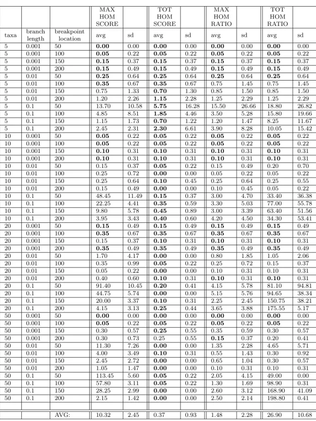
The results are summarized in Table1(for the 2-block experiment) and Table2(for the multiple-block experiment.) For each parameter combination, we report average and standard deviation of the breakpoint error (ranging over the 20 replicates). In each row of the tables, the smallest average (ranging across the four optimization models) is shown in bold. At the foot of each table we provide average-of-averages and average-of-standard-deviations.
5.1 Analysis of experiments
Both experiments indicate that, overall, Total Homoplasy Score is the best algorithm, then Max Homoplasy Ratio, then Max Homoplasy Score, and finally Total Homoplasy Ra-tio. The average-of-averages shown at the foot of each table emphasize this. A number of obser-vations can be made:
– Across both experiments, and across most parameter combinations, Total Homoplasy Score achieves an average error across the 20 replicates of (much) less than 1.0. This means that To-tal Homoplasy Score is almost always inferring breakpoint locations that are within one informative site of the their correct locations. In the 2-block experiment, the only exception to this is several of the (t, bℓ) = (5, 0.1) parameter combinations, which have slightly higher aver-ages and standard deviations. (These combinations also disrupt the other optimization models.) We believe this is because trees with long branches and few taxa produce very little phyloge-netic signal enabling the separation of regions generated by different trees. In the multiple-block experiment, the (5, 0.1) combinations behave similarly, but there (50, 0.001) combinations also cause the average to rise marginally above 1.0.
– In both experiments, many of the parameter combinations cause both Max Homoplasy Score and Total Homoplasy Ratio to suffer very large breakpoint errors. Interestingly, in both experiments these huge errors only occur when branch lengths are long (0.1). We reflect below on the reasons for this, which are different for the two models.
– Overall, the performance of Max Homoplasy Ratio seems somewhat correlated with To-tal Homoplasy Score. Unlike the other two optimization models, neither of these models produces any spectacularly large breakpoint errors.
– In both experiments, for extremely short branch lengths (0.001) all models exhibit similar performance. This is connected to the fact that, for such extremely short branch lengths, an alignment typically contains very few informative sites. To give a concrete example: in the 2-block experiment, for bℓ = 0.001, an alignment generated with t = 5 might contain only 1 informative site per block, rising to at most 15-20 for t = 50. Given the definition of breakpoint error this means that there are many sites that do not contribute to the error, so the breakpoint error will be limited in magnitude irrespective of the exact optimisation criterion being used. – Close observation of the full experimental results, available on the CutAl GitHub page, for
Max Homoplasy Score shows that this criterion tends to underestimate the size of the largest block. In the 2-block experiments, this is particularly evident for bℓ = 0.1, where for location = 50, 100, 150 the inferred breakpoint is nearly always to the right of the correct position (e.g., for t = 50 it is always between 150 and 205, irrespective of the true position of the breakpoint). This phenomenon is also detectable for t = 50, bℓ = 0.01 and location = 50, where the inferred breakpoint is on average more than 10 informative sites to the right of the correct beakpoint (cf. Table1). This behavior is not surprising, as the goal of this problem is to minimize the homoplasy in the block with the most homoplasy (which usually coincides with the largest block). Thus, solutions of Max Homoplasy Score will tend to reduce the size of the largest block to reduce its homoplasy (while increasing the homoplasy of the blocks flanking the largest block). The incentive to do so is stronger when the homoplasy within the largest block is much bigger than the homoplasy in its flanking blocks, a difference that we expect to be particularly pronounced when the tree has very long (or many) branches (for large values of bℓ and/or t) or when the blocks have very different sizes. As expected, when the true blocks have similar sizes (e.g., for location = 200 in the 2-block experiment) this phenomenon has a tendency to disappear (cf. Table1).
– Total Homoplasy Ratio suffers from a problem that can be seen as a very severe inverse of that of Max Homoplasy Score: whenever per-site substitutions are frequent (in our experiments for bℓ = 0.1), the partitions it produces tend to consist of a single large block and a number of smaller blocks. For example, for the extreme case where t = 50 and bℓ = 0.1: (a) in the 2-block experiments, all of the partitions returned consist of a block of 1 or 2 sites, and a block containing the remaining sites; (b) in the multi-block experiments, all partitions consist of a number of blocks of 1 or 2 sites, and a single block with all the remaining sites. (2-site blocks are much rarer than 1-site blocks, as they only occur in <5% of these partitions.) The reason why this happens is that when substitutions are frequent—in other words, when the sites are saturated with substitutions—each block will have a high homoplasy ratio, regardless of whether the MP tree for that block accurately describes its evolution, or not. The only exception to this are very small blocks consisting of few sites, in which case it becomes possible to find a tree that explains those few sites with little or no homoplasy (e.g., 1-site blocks always have homoplasy ratio 0). So, in order to minimize the sum of homoplasy ratios for k blocks, it becomes convenient to have k − 1 small blocks with very small homoplasy ratios and one large block with high homoplasy ratio, rather than to have a realistic block partition where each block has an anyway high homoplasy ratio. This is a very serious issue for Total Homoplasy Ratio, which results in very high breakpoint errors whenever the alignment is saturated with substitutions.
6 Discussion
Inference methods estimating quantities that are paramount to our understanding of molecular evolution (e.g. positive selection and branch length estimates) can be seriously mislead by recom-bination. Since no theory yet exists to define the amount of recombination that can be borne by these methods to still produce the correct answer, a safer way to deal with the problem is to restrict one’s attention to the analysis of non-recombinant loci.
In this article, we investigated several different parsimony-based approaches towards detecting recombination breakpoints in a multiple sequence alignment, and we described algorithms for each of our formulations. These algorithms have been implemented and, via tests on simulated data, we have identified a number of important weaknesses of two of these approaches. Our experiments also
MAX HOM SCORE TOT HOM SCORE MAX HOM RATIO TOT HOM RATIO taxa branch length breakpoint
location avg sd avg sd avg sd avg sd
5 0.001 50 0.00 0.00 0.00 0.00 0.00 0.00 0.00 0.00 5 0.001 100 0.05 0.22 0.05 0.22 0.05 0.22 0.05 0.22 5 0.001 150 0.15 0.37 0.15 0.37 0.15 0.37 0.15 0.37 5 0.001 200 0.15 0.49 0.15 0.49 0.15 0.49 0.15 0.49 5 0.01 50 0.25 0.64 0.25 0.64 0.25 0.64 0.25 0.64 5 0.01 100 0.35 0.67 0.35 0.67 0.75 1.45 0.75 1.45 5 0.01 150 0.75 1.33 0.70 1.30 0.85 1.50 0.85 1.50 5 0.01 200 1.20 2.26 1.15 2.28 1.25 2.29 1.25 2.29 5 0.1 50 13.70 10.58 5.75 16.28 15.50 26.66 18.80 26.82 5 0.1 100 4.85 8.51 1.85 4.46 3.50 5.28 15.80 19.66 5 0.1 150 1.15 1.73 0.70 1.22 1.20 1.47 8.25 11.67 5 0.1 200 2.45 2.31 2.30 6.61 3.90 8.28 10.05 15.42 10 0.001 50 0.05 0.22 0.05 0.22 0.05 0.22 0.05 0.22 10 0.001 100 0.05 0.22 0.05 0.22 0.05 0.22 0.05 0.22 10 0.001 150 0.10 0.31 0.10 0.31 0.10 0.31 0.10 0.31 10 0.001 200 0.10 0.31 0.10 0.31 0.10 0.31 0.10 0.31 10 0.01 50 0.15 0.37 0.05 0.22 0.15 0.49 0.20 0.70 10 0.01 100 0.25 0.72 0.00 0.00 0.05 0.22 0.05 0.22 10 0.01 150 0.25 0.64 0.10 0.45 0.25 0.64 0.25 0.55 10 0.01 200 0.15 0.49 0.00 0.00 0.10 0.45 0.05 0.22 10 0.1 50 48.45 11.49 0.15 0.37 3.00 4.70 33.40 36.38 10 0.1 100 22.25 4.41 0.35 0.59 3.30 5.03 77.00 55.78 10 0.1 150 9.80 5.78 0.45 0.89 3.00 3.39 63.40 51.56 10 0.1 200 3.95 3.43 0.40 0.60 4.20 4.50 34.30 53.41 20 0.001 50 0.15 0.49 0.15 0.49 0.15 0.49 0.15 0.49 20 0.001 100 0.35 0.67 0.35 0.67 0.35 0.67 0.35 0.67 20 0.001 150 0.15 0.37 0.10 0.31 0.10 0.31 0.10 0.31 20 0.001 200 0.35 0.49 0.35 0.49 0.35 0.49 0.35 0.49 20 0.01 50 1.70 4.17 0.00 0.00 0.80 1.85 1.05 2.06 20 0.01 100 0.35 0.99 0.05 0.22 0.25 0.72 0.15 0.37 20 0.01 150 0.05 0.22 0.00 0.00 0.10 0.31 0.10 0.31 20 0.01 200 0.40 0.60 0.10 0.31 0.10 0.31 0.10 0.31 20 0.1 50 91.40 10.45 0.20 0.41 4.15 5.78 81.10 94.81 20 0.1 100 44.75 5.74 0.00 0.00 5.15 5.76 94.65 38.34 20 0.1 150 20.00 3.37 0.10 0.31 2.25 2.45 150.75 38.21 20 0.1 200 4.15 3.13 0.25 0.44 3.65 3.88 175.55 5.17 50 0.001 50 0.00 0.00 0.00 0.00 0.00 0.00 0.00 0.00 50 0.001 100 0.05 0.22 0.05 0.22 0.05 0.22 0.05 0.22 50 0.001 150 0.30 0.57 0.25 0.55 0.35 0.59 0.30 0.57 50 0.001 200 0.30 0.73 0.25 0.55 0.15 0.37 0.20 0.41 50 0.01 50 11.30 7.26 0.00 0.00 1.35 2.28 4.65 5.71 50 0.01 100 4.00 3.49 0.10 0.31 0.55 1.43 0.30 0.92 50 0.01 150 2.45 2.72 0.00 0.00 0.65 1.04 0.30 0.57 50 0.01 200 1.05 1.47 0.00 0.00 0.10 0.31 0.10 0.31 50 0.1 50 113.45 5.60 0.05 0.22 2.05 4.15 49.00 0.00 50 0.1 100 57.80 3.11 0.05 0.22 1.30 1.69 98.90 0.31 50 0.1 150 28.25 2.99 0.00 0.00 2.60 3.12 168.90 41.09 50 0.1 200 2.15 1.42 0.00 0.00 2.50 2.14 198.80 0.41 AVG: 10.32 2.45 0.37 0.93 1.48 2.28 26.90 10.68
Table 1 2-block experiment
suggest that the best formulation of block partitioning, among those that we have considered, is Total Homoplasy Score. We note that this formulation is closely linked to that of Mdl (Ané 2011): it is easy to see that for any value of the penalty parameter against the number of blocks in Mdl, there exists a value of the parameter b for Total Homoplasy Score that would yield the same block partition.
The work in this paper has led to several interesting open computational problems which could be studied in further research. First of all, a fundamental question is whether one can decide in polynomial time whether two blocks are mergeable, i.e., whether they can be combined into a single block without increasing the total homoplasy. Simply computing the homoplasy for each block and
MAX HOM SCORE TOT HOM SCORE MAX HOM RATIO TOT HOM RATIO taxa branch
length blocks avg sd avg sd avg sd avg sd
5 0.001 3 0.03 0.11 0.03 0.11 0.03 0.11 0.03 0.11 5 0.001 4 0.30 0.44 0.30 0.44 0.30 0.44 0.30 0.44 5 0.001 5 *** *** *** *** *** *** *** *** 5 0.001 6 *** *** *** *** *** *** *** *** 5 0.01 3 0.80 1.22 0.60 1.12 0.68 1.13 0.60 1.12 5 0.01 4 1.33 1.34 1.30 1.28 1.20 1.08 1.20 1.08 5 0.01 5 0.93 1.16 0.88 1.18 0.88 1.18 0.88 1.18 5 0.01 6 1.31 1.27 1.31 1.27 1.31 1.27 1.31 1.27 5 0.1 3 7.58 8.30 3.88 6.02 6.38 9.38 10.25 10.47 5 0.1 4 4.13 4.63 2.93 3.99 6.85 8.07 13.40 7.97 5 0.1 5 5.93 4.31 4.24 5.97 6.10 6.19 23.23 13.64 5 0.1 6 4.23 3.37 3.38 4.05 8.25 5.57 23.60 9.18 10 0.001 3 0.50 1.08 0.50 1.08 0.50 1.08 0.50 1.08 10 0.001 4 0.25 0.36 0.25 0.36 0.25 0.36 0.25 0.36 10 0.001 5 0.56 0.76 0.56 0.76 0.56 0.76 0.56 0.76 10 0.001 6 0.37 0.42 0.37 0.42 0.37 0.42 0.37 0.42 10 0.01 3 0.83 1.32 0.30 0.91 1.18 2.89 1.05 2.86 10 0.01 4 1.53 2.83 0.72 2.09 0.42 0.66 0.42 0.67 10 0.01 5 0.41 0.46 0.15 0.19 1.10 1.54 1.00 1.73 10 0.01 6 1.28 1.66 0.63 1.05 1.17 1.78 0.64 0.97 10 0.1 3 17.03 15.03 0.63 0.93 5.13 6.71 80.03 33.37 10 0.1 4 17.62 11.88 0.55 0.60 4.40 3.31 86.60 32.55 10 0.1 5 14.33 8.27 0.34 0.34 6.54 11.32 80.95 21.78 10 0.1 6 7.27 5.41 0.33 0.31 6.35 7.04 96.84 21.16 20 0.001 3 0.80 1.37 0.80 1.37 0.85 1.36 0.85 1.36 20 0.001 4 0.77 0.91 0.77 0.91 0.72 0.91 0.72 0.91 20 0.001 5 0.88 0.76 0.88 0.76 0.88 0.76 0.88 0.76 20 0.001 6 0.66 0.60 0.66 0.60 0.66 0.60 0.66 0.60 20 0.01 3 1.13 1.19 0.10 0.21 0.70 0.80 0.45 0.69 20 0.01 4 1.37 1.18 0.17 0.28 1.27 3.97 0.60 1.24 20 0.01 5 1.14 1.65 0.18 0.18 1.23 3.00 1.50 3.86 20 0.01 6 0.63 0.61 0.11 0.15 0.72 1.31 0.45 0.87 20 0.1 3 39.03 20.64 0.28 0.34 1.78 2.11 121.48 35.40 20 0.1 4 24.80 11.97 0.08 0.15 2.78 1.64 144.58 42.29 20 0.1 5 18.70 9.01 0.14 0.19 4.08 6.74 148.66 37.15 20 0.1 6 13.41 7.02 0.09 0.12 2.83 1.72 131.72 35.70 50 0.001 3 0.83 1.40 0.80 1.41 0.80 1.41 0.80 1.41 50 0.001 4 1.65 1.83 1.35 1.59 1.28 1.59 1.28 1.59 50 0.001 5 1.60 1.86 1.59 1.87 1.56 1.88 1.55 1.89 50 0.001 6 1.70 1.68 1.66 1.71 1.52 1.40 1.48 1.41 50 0.01 3 6.88 5.85 0.13 0.22 1.05 1.16 1.55 3.69 50 0.01 4 5.57 6.48 0.15 0.20 0.73 0.68 0.80 1.45 50 0.01 5 2.76 2.51 0.13 0.21 1.03 0.89 1.90 6.83 50 0.01 6 1.44 0.68 0.09 0.14 0.91 1.00 0.19 0.21 50 0.1 3 52.08 26.90 0.13 0.22 3.20 3.37 135.93 56.92 50 0.1 4 29.05 18.99 0.07 0.14 1.07 0.83 162.22 44.56 50 0.1 5 23.43 10.96 0.05 0.10 1.66 1.04 149.60 39.10 50 0.1 6 18.12 7.31 0.10 0.15 2.04 1.41 149.65 34.72 AVG 7.32 4.76 0.75 1.04 2.07 2.48 34.42 11.28
Table 2 Multiple-block experiment
the combined block does not work (unless P = NP) because computing the homoplasy of a block is NP-hard. Hence, a more advanced strategy would need to be developed. A slightly different but equally interesting question is the following. Suppose we are given a tree with minimum homoplasy for the first j columns of an alignment. Can we decide in polynomial time whether the same tree has minimum homoplasy for the first j + 1 columns? We would also like to reiterate here a well-known open problem in the area, which is strongly related to the studied problems. Does there exists an FPT algorithm deciding whether there exists a tree with homoplasy at most h for a given alignment of nonbinary characters, when h is the parameter? In particular, this problem (the h-near perfect phylogeny problem) is even open for 3-state characters. Answering this question positively would also extend the FPT results in this paper to nonbinary characters.