HAL Id: hal-01562908
https://hal.archives-ouvertes.fr/hal-01562908
Submitted on 20 Apr 2018HAL is a multi-disciplinary open access
archive for the deposit and dissemination of sci-entific research documents, whether they are pub-lished or not. The documents may come from teaching and research institutions in France or abroad, or from public or private research centers.
L’archive ouverte pluridisciplinaire HAL, est destinée au dépôt et à la diffusion de documents scientifiques de niveau recherche, publiés ou non, émanant des établissements d’enseignement et de recherche français ou étrangers, des laboratoires publics ou privés.
flow vs cross-barrier gradients
Damien Sous, Lise Petitjean, Frederic Bouchette, Vincent Rey, Samuel Meulé,
François Sabatier
To cite this version:
Damien Sous, Lise Petitjean, Frederic Bouchette, Vincent Rey, Samuel Meulé, et al.. Groundwater fluxes within sandy beaches: swash-driven flow vs cross-barrier gradients. Coastal Dynamics 2017, Jun 2017, Helsingor, Denmark. �hal-01562908�
GROUNDWATER FLUXES WITHIN SANDY BEACHES: SWASH-DRIVEN FLOW VS CROSS-BARRIER GRADIENTS
Damien Sous1, Lise Petitjean1, Frédéric Bouchette2, Vincent Rey1, Samuel Meulé3 and François Sabatier3
Abstract
This communication reports on a field experiment carried out on a microtidal beach in Camargue, France. The analysis is built on the initial work presented by Sous et al. (2016) on swash-groundwater dynamics. The analysis of a cross-shore network of buried pressure sensors allows to monitor the watertable dynamics over the full 2013-2014 winter season. The pressure head gradients are observed to be primarily seaward, forced by a higher level at the landward boundary. The groundwater flux is driven by the relative fluctuations of Still Water Level and inland elevations. Rain and tides have a little effect. A nearly isolated groundwater circulation is driven by wave activity below the swash zone whatever the overall watertable gradient. Estimations of beach groundwater discharge over the Gulf of Beauduc reveal the importance of beach groundwater in the exchanges between coastal aquifer and open sea.
Key words: swash zone, groundwater dynamics, watertable gradients, seasonal survey, field experiment
1. Introduction
Groundwater fluxes through sedimentary beaches or barriers are expected to play a great role in the exchanges of fresh and salt water between open sea, lagoons and aquifers (Elad et al. 2016, Hamada et al. 2017) as well as in the transport of dissolved nutrients and pollutants (Sawyer et al. 2014). From field measurements in a microtidal sandy beach, Sous et al. (2016) recently demonstrated the presence of a groundwater circulation cell under the swash zone. These observations raised once again the key question of the effect of the landward fluctuations of the watertable on the beach groundwater flows. This debate has been earlier fed in particular by the contrasting results provided by the experiments of Turner et al. (2015) and the numerical simulations of Li and Barry (2000). They both observed infiltration at the upper swash and exfiltration at the lower swash, regardless the artificially imposed seaward- or landward-directed hydraulic gradients across the barrier. However, Turner et al. (2015) showed a groundwater circulation under the swash zone nearly isolated from the artificial back-barrier fluctuations while Li and Barry (2000) stated that the inland watertable elevation affects the location of the divergence point at the top of the swash zone.
Using an extensive network of buried pressure sensors from the surf zone to the dune base, the present field study brings new insight on this issue. The second section of the communication is dedicated to the description of the field experiments while the third section presents the results, including a particular focus on a submersion storm event. Conclusive remarks and prospects are given in the last section.
2. Experiments
This work is a part on a larger scale high resolution hydro-morphodynamic field campaign (ROUSTY 2014) conducted from November 2014 to February 2015 on the Rousty beach (Camargue, France). The field site is an open and linear microtidal wave dominated beach oriented West-East. The sedimentary material consists of a fine sand ~ 200µm in size. The hydraulic conductivity is 0.016 cm/s (Sous et al., 2016). Main geomorphic features are a 50-70 m wide mild slope beach, an uneven barrier dune up to 5 m high, and a double barred system within 5 m of water depth.
1
Université de Toulon, CNRS/INSU, IRD, MIO,UM110, 83051 Toulon Cedex 9, France. sous@univ-tln.fr
2
GEOSCIENCES Montpellier, Université de Montpellier II, Montpellier, France
3
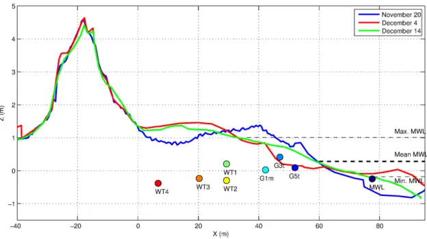
The instrumentation used here consists in a cross-shore network of buried pressure sensors depicted in Figure 1. Three synchronized high-frequency (10Hz) pressure sensors (named G1m, G3t and G5t) are deployed under the swash zone during a 24h period corresponding to the decay of a moderate storm event (see Sous et al. 2016 for details about the full swash zone experiment). In addition, five autonomous sensors are buried under the surf zone (MWL) and inland within the upper beach (WT1 to WT4) to measure groundwater at lower frequency (5Hz for MWL and 0.007Hz for WTs). Measured data are averaged over 30min time windows. Each sensor was repeatedly positioned by DGPS and tacheometer during the experiment, and calibrated in laboratory basin both before and after the experimental campaign. The sensors are protected by a sediment net to prevent sediment infiltration and sensor membrane damage (Turner and Nielsen, 1997). Note that WT1 and WT2 measurements stop on December, 4 (battery limitations). Offshore wave and water level (named SWL) are provided by an additional ADCP in 7m depth.
Topo-bathymetric surveys have been performed all along the experiments. Three beach profiles (Nov. 20, Dec. 4 and Dec. 14) are plotted in Fig. 1 to help the results discussion.
Figure 1. Experimental setup and three selected cross-shore beach profiles. G1m, G3t and G5t are high-frequency sensors only deployed for the storm of Dec. 12-14 while WT1 to WT4 are deployed for the full experiment (Nov. 20,
2014 to Feb. 10, 2015). Minimal, mean and maximal values of the Mean Water Level over the whole experiment are computed from the MWL sensor.
A number of inter-connected lagoons are present inland in the Parc Naturel Regional de Camargue. The exchanges between lagoons are fully controlled by a system gates and channels such as there is no direct relationship between rainfall and back-barrier lagoons levels. The data analysis will thus be mainly carried out considering the inner boundary conditions measured at WT4 sensor.
3. Results
Sous et al. (2016) analyzed a high-resolution data subset in the swash zone. This study was limited in time to a single winter storm and focused on the swash-groundwater interactions. Here, we extend this analysis to the whole experiment in order to highlight the respective role played by the swash dynamics and the inland watertable gradients in the groundwater circulation through the beach.
3.1. Data overview
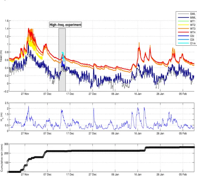
The pressure head data recovered during the whole experiment is depicted in Fig. 2. The 30-min time averaged free surface elevation in the inner surf zone (MWL sensor) show significant fluctuations, which mainly result from the combination of large scale SWL oscillations, tide and wave activity (wave setup). The most important driver is clearly the SWL which shows oscillations up to 1m in response to the variations of atmospheric pressure and other large scale coastal features. The tide is between 10 and 30cm, typical of micro-tidal conditions encountered in this region of the Mediterranean basin. The wave setup measured at MWL (indeed the difference between the head at MWL and the offshore time-averaged elevation SWL) sensors is relatively small, with a maximal value about 0.15m.
3.1.2. Groundwater dynamics
The response of the beach aquifer is monitored thanks to the network of buried cross-shore sensors (see Fig. 2). The first observation is that the upper beach head, measured by sensors WT3-4 is nearly systematically the greater. The watertable is thus higher than the surf zone MWL, of the order of 20-40cm. This is most likely related to the presence of a high watertable level at the inland boundary, forced by the back-barrier lagoons (Vaccarès lagoon). Such observation may correspond to the well-know superelevation of the watertable widely observed in other sites (see Turner 1998, Raubenheimer et al. 1999, Kang and Nielsen 1994). Note that the respective roles of wave forcing and large scale gradients on the watertable elevation are still poorly documented in the literature, which is part of what is driving the present study.
Two additional typical observations can be performed. First, the sand soil acts as a low-pass filter. The day-to-week scale fluctuations of the Still Water Level easily propagates within the beach, inducing watertable oscillations of the same order of magnitude. At higher frequency, the tidal fluctuations are damped when propagating into the beach aquifer (Turner et al. 1997, Turner 1998, Raubenheimer et al. 1999). In our microtidal site, the tide effect becomes barely measurable for the upper beach sensors (WT3 and WT4). Second, comparison between WT1 and WT2 sensors located at the same cross-shore position shows that the pressure field is very close to the hydrostatic equilibrium below the upper beach, with departure from hydrostaticity about 1%. This is in contrast with the measurements performed in the swash groundwater (Sous et al. 2016) for which the deviation from the hydrostatic balance can reach 20% and thus induces significant vertical flows below the beach face but confirms that, above the action zone of the swash, the pressure field is nearly hydrostatic and the related groundwater motion are horizontal.
The general trend is that the watertable follows the low frequency evolution of the SWL which is clearly the dominant driver of beach aquifer oscillations. This simple relationship is however affected by a number of secondary mechanisms. One notes first that the watertable can rise independently from free surface levels and/or wave activity, see e.g. November 25, December 4-5 or January 21. This is largely explain by the rain input, plotted in Fig. 2, bottom plot. It is remarkable that in most cases, the watertable rising is much greater than the rainfall amount. This probably indicates a cumulative effect of the direct water input on the beach and the lateral loading from back-barrier lagoons which drain water from the inland watershed. For some events, e.g. November 28-29 and January 19, both MWL setup and rainfall combine to elevate the watertable, which makes difficult to identify their relative contributions.
It is also observed that the relation between MWL and watertable risings depends on the initial elevation. During low level periods, the events of rapid MWL increase induce small response of the watertable. This is for instance observable for the events of December 9 and 27 or January 12, for which MWL rising about 20 to 30 cm only produce watertable rising of few centimeters. By contrast, when the overall water level is initially high, or when the MWL increase is long enough (over several days), the rising of MWL and watertable are generally of the same order of magnitude, see November 28, December 13, January 15-16 or February 3. While not fully understood, this observation should be related to beach saturation issues, the beach acting as a porous reservoir.
Figure 2. Overview of the recovered data during the winter season: pressure head (Top), deep-water wave height (Middle) and cumulative rain (Bottom). The grey box indicates the high-frequency deployment.
3.2. Submersion event
A particular attention is thus paid on the period from November 27 to December 3 during which the combined effects of wave activity and strong SWL/MWL setup lead to a major submersion event. Figure 3 depicts the evolution of pressure heads within the sand (top plot), the deep-water wave height (middle plot) and the rainfall (bottom plot) over this selected period.
The analysis of the groundwater behavior during the submersion should be made with caution, as both beach face and upper beach experienced very strong morphological evolution. This is clearly visible when comparing the morphological surveys performed before and after the storm (bed levels in blue and red lines in Fig. 1). In addition to this overall morphological evolution, note that the upper beach is usually covered by aeolian sand three-dimensional mobile deposits, with amplitude and extension about 20-50cm and few meters, respectively. These wind-induced bedforms, visible in Fig. 1 on the Nov. 20 profile, are made of loose aeolian sand which moves under wind action but are generally erased during large submersion events.
The initial situation before the submersion event, shown in Fig. 2, corresponds a slightly titled watertable below the upper beach, with all WT's sensors indicating close but seaward decreasing pressure heads. The moderate risings of the watertable on November 22 and 25 are associated to wave event and rainfall activity, respectively.
A series of successive phases is now selected to depict the submersion process, see Phases S1 to S6 in Fig. 3. During the night of December 27-28 (Phase S1, see Fig. 3), a rapid increase of the pressure head is observed for each WTs sensors. The rise is stronger seaward (38cm for WT1 and 17cm for WT4). This event occurs during a period of overall increase of wave activity (See Fig. 2 for an overview) and rising tide, but the relative suddenness of the watertable rise is remarkably rapid considering the slow evolution of the forcings. A careful observation of Phase S1 in Fig. 3 reveals that the watertable rise is not regular but rather results from successive abrupt increases followed by steady phases. Spectral analysis (Sous et al. 2016) indicates that the Rousty beach is dissipative under storm conditions. The swash zone is clearly dominated by low-frequency infragravity motion. Such long waves are able to successively load the beach aquifer, which explain the sequential watertable loading observed during Phase S1. The comprehensive characterization of the saturation process, including capillary fringe dynamics, would require a much more sophisticated instrumental apparatus (Heiss et al. 2014).
A nearly 24h steady phase (Phase S2, see Fig. 3) is then observed during the morning of November 28. The pressure head measured by WT1-2 sensors is close to the pre-storm bed level at this location, which indicates that the beach is here probably fully saturated and the watertable has risen up to the bed. The facts that the watertable remains coupled with the sand bed for several hours and that the observed decoupling events are rapidly compensated in one or few successive steps indicate the regular input of IG-driven swash events. Landward (WT3-4), the pressure head does not appear to precisely coincide with the pre-storm bed level, the watertable remains few centimeters below the sand. But according to the estimation of Turner and Nielsen (1997), the capillary fringe in Rousty beach should be several tens of centimeters high, so the sand bed itself is very close to saturation.
Phase S3 corresponds to a strong rise of the water level, induced by the combined effects of increasing wave activity and incoming tide. WT1-2 sensors shows a moderate increase in pressure head followed by a larger decay (Phase S4). As the general morphological trend is a landward shift of the berm during the storm, it is likely that this rising correspond to the passage of the berm apex. The sand remains fully saturated due to the regular income of submersion infragravity waves, and the pressure measurement performed here each 2,5 min simply follows the evolution of the sand bed. During the same phase, the upper beach sensors WT3-4 show a much stronger pressure increase, of the order of 30cm. A steady phase is thus observed (Phase S4), during which both WT3 and WT4 sensors shows similar heads. This probably indicates that the runnel is now filled with water.
Later on, a 31h-long phase (Phase S5, Nov. 29, 19:00 to Nov. 30, 03:00) is observed during which the time-averaged component of pressure head is remarkably steady under the berm (WT1-2), with a watertable about 20cm below the sand surface. Regular fluctuations, of the order of 10cm, are superimposed to this steady mean value. These fluctuations are typical of the IG-driven motions in the upper swash observed by Sous et al. 2016 for another storm event (see also next section for further details). In the upper beach, the rapid head fluctuations observed for WT2 indicate probably capillary processes, with the watertable oscillating between the sand bed and a lower equilibrium position. A finer analysis would require higher temporal resolution. Landward, WT4 is more stable. The last phase (Phase S6) is an ensemble slow lowering of the watertable affected by tidal fluctuations and episodic peaks.
Figure 3. Groundwater dynamics during the Nov. 28 – Dec. 1 submersion event. Six phases numbered from S1 to S6 are selected to help the discussion. Top plot: pressure head, middle plot: deep water wave height, bottom plot:
cumulative rainfall.
3.3. Swash-driven vs watertable gradients
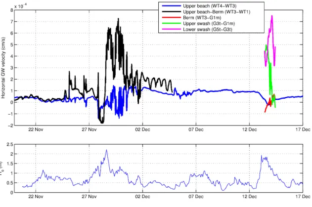
Fig. 1 shows that pressure gradient between upper beach watertable (WT3-4 sensors) and inner surf zone (MWL) are overwhelmingly negative (landward), i.e., following Darcy's assumptions, groundwater follows the decreasing potential and flows toward the open sea. While more limited in time, WT1-2 measurements confirm this dominant trend, induced by the back-barrier lagoon forcing at the landward boundary. The head gradients between upper beach (WT3-4) and MWL are of the order of 1%, fluctuating under the action of wave activity, sea level variations, inland boundary condition and rainfall (see Fig. 2). Darcy's law states that the horizontal groundwater velocity is inversely proportional to the cross-shore head gradients, the proportionality factor being K the hydraulic conductivity. Using such calculation between selected measurement points, horizontal groundwater velocities are computed and depicted in Fig. 4, for the November 20 to December 17 period. The present analysis is focused on the sole horizontal component. Vertical motions are expected to be very weak as the pressure distribution is nearly hydrostatic everywhere in the beach except under the swash zone (Sous et al. 2016).
Figure 4. Top plot: horizontal Darcy groundwater velocity between sensor pairs (positive velocity is seaward). Bottom plot: deep water wave height.
The reference groundwater state in Rousty beach during the 2014-2015 winter season can be observed for instance in Fig. 4 between November 20 to 28 and December 2 to 12. It is characterized by a very small seaward velocity, nearly the same for the WT4-3 and WT3-1 sensors pairs.
The effect of rainfall alone on this reference situation is observed on November 25 and 26-27, and later on December 6. As exposed herein before, the rainfall input rises and slightly tilts the watertable (Fig. 2) but the associated seaward groundwater velocity remains weak (Fig. 4).
The main drivers of groundwater gradients are the combined effects of mean water levels at the boundaries and wave at the beach face. For a better understanding of their interactions, a particular attention is paid now on the two dominant storms in terms of waves, levels and available instrumentation. The first storm is the submersion event on Nov. 28 to Dec. 1 described above, named Storm 1, while the second storm is the swash-monitored one on December 13-14, named Storm 2.
The first stage of Storm 1 (Phase S2 in Fig. 3) is a beach submersion characterized by a reversal of the head gradient and a landward groundwater flux all over the studied cross-shore profile. The associated negative velocity remains weak, about 1.5.10-6 m/s (Fig. 4), and is maximal under the berm. As exposed
previously, Phase S2 corresponds to a submersion event where the beach is probably fully saturated (or even partly immersed). In this case, the groundwater head gradients are related to the bed morphology: the head is maximal under the berm and groundwater should flow toward lower zones of the upper beach. During the storm retreat (from S3 Phase in Fig. 3), the groundwater under the berm flows seaward and the velocity strongly increases up to 7.10-6 m/s (Fig. 4) while further landward the velocity fluctuates around
zero below the upper beach. Such difference between berm and upper beach gradients is remarkable. It is explained by the fact that, in the no-wave no-rain reference state, the watertable should show a regular negative slope from the landward high-level boundary down to the open sea (or exit point if decoupled). The effect of wave action, here mainly IG waves in the swash zone, is to maintain a higher watertable level under the berm, relatively to the elevation it would have had without wave. This corresponds to the classical hump shape of the watertable observed by other authors (e.g. Lanyon et al. 1982, Sous et al. 2013), applied here in the particular context of a high landward watertable boundary condition.
From December 2, the wave activity decreases. The groundwater returns to its reference state, mainly controlled by the gradient between landward condition and MWL at the beachface. They both follow a similar decrease only affected by tidal fluctuations. The general fall of watertable and open sea levels is observed up to the storm of December 12-14. The only deviation is due to the rain input on December 5, which rises the upper beach watertable of about 20cm but does not significantly increase the groundwater velocity below the upper beach (data under the berm is unfortunately no more available).
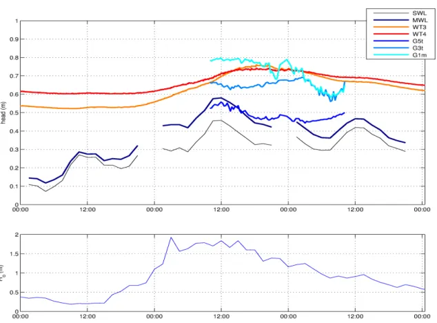
Storm 2 has been detailed in terms of swash zone processes by Sous et al. (2016) and is here further analyzed to understand the relation between swash-driven and cross-barrier watertable gradients (Fig. 5). Let us recall here that Sous et al. (2016) observed, (i), a time-averaged anti-clockwise circulation cell and, (ii), at shorter time scale a typical groundwater circulation pattern associated to incoming IG-driven swash events. In the present study, we only consider the horizontal component of the motion. The initial situation on December 12 depicted in Figs. 4 and 5 shows the reference groundwater situation in Rousty beach, i.e. a slow seaward groundwater flow associated to a titled upper beach watertable due to a higher landward level. The storm arrival during the evening of Dec. 12 forces a higher MWL at the beachface, progressively flattens the upper beach watertable and inhibits the seaward flow. The high-frequency groundwater measurements start near the storm apex on Dec. 13 around 12:00. The groundwater gradients observed under the swash zone are much higher than below the upper beach, inducing seaward velocities five to ten times greater than their upper beach counterparts. It is remarkable to note that, at least at the spatial resolution of the present experimental setup, these strong head gradients at strictly limited to the swash zone. The head at the top of the swash zone (G1m sensor) is just slightly greater than the upper beach water table one, only inducing a small landward flux. The storm starts to decrease from Dec. 13, 12:00. The swash zone pressure heads remain nearly steady until the early morning Dec. 14 and then starts to fall (see Sous et al. 2016 for a finer analysis) while the upper beach watertable is still rising and flattens (the slope even shows a slight reversal during the evening of Dec. 13). This highlights the time lag between beach face and upper beach groundwater processes. The watertable gradient under the berm (between G1m and WT3) decreases as the upper beach watertable rises and reverses as the swash zone level starts to fall during the night of Dec. 13-14. It is again noted that, for the whole considered event, the cross-berm groundwater flux (being either positive or negative) remains one order of magnitude smaller than the seaward flow under the swash zone. During Dec. 14 and later on, the watertable progressively falls back to its reference state associated to slow seaward flux within the sand soil.
Let us know compare and relate these two storms. Storm 1 was characterized by larger waves and higher MWL. However, in terms of swash-groundwater velocities, the situation described in Storm 1 Phases S4 and S5 is nearly the same that for Storm 2. Measurements performed under the swash zone, i.e. between WT1 and G1m and between G1m and G5t for Storms 1 and 2, respectively, shows similar seaward groundwater flows with the same order of magnitude. Following the study of Sous et al. 2016 focused on a single event, this experiment confirms in the field the laboratory observation of Turner et al. 2015 and the numerical simulation of Li and Barry (2000): a typical seaward groundwater circulation pattern under the swash zone. In addition, the present analysis allows to describe, for the first time in the field, the role played by upper beach watertable gradients. If the inland watertable is low, a divergence point can observed near the top of the swash zone (Storm 2 apex), but it can be smoothed or inexistent with higher inland watertable. What is important is that, whatever the upper beach watertable situation, the waves action at the swash zone are able to drive a localized swash-groundwater circulation. This circulation is about one order of magnitude stronger than the typical groundwater flux under the upper beach.
Figure 5: Groundwater dynamics during a three days period (Dec. 12 to Dec. 14) associated with a significant wave event. Swash-zone groundwater data (G1m, G3t, G5t sensors) are extracted from the analysis presented in Sous et al.
2016.
The observations performed during the 2014-2015 winter season in Rousty beach can be summarized as follows:
- the general trend is a slow (about 1.10-6 m/s) seaward groundwater flow driven by a high-level landward
boundary condition in back-barrier lagoons;
- rainfall events induce an overall rise of the watertable (generally greater than the rain input), but do not significantly increase of groundwater discharge (for the considered events);
- storm events, associated to increased wave energy (Ho>1.5m) and setup of MWL, are able to rise the watertable under the berm inducing, (i), a flattening or even a reversal of the watertable slope below the upper beach and, (ii), a seaward groundwater flow under the swash zone typically one order of magnitude stronger than its upper beach counterpart;
3.4. Discussion on beach groundwater discharge
The groundwater dynamics fluctuates under the action of waves, sea and inland levels variations, rainfall and beach morphology. An attempt is made here to estimate the exchanged volumes through the beach. One must keep in mind the limitations of the present experimental setup, in particular the lack of spatial and temporal resolution, the fact that vertical motions are neglected and the unknown total depth of beach aquifer. This latter would require dedicated seismic and/or core sampling measurements, but is here estimated to be of the order of 10m.
The exchanges related to the swash-groundwater circulation have been calculated by Sous et al. (2016) for a 1.5m deep sand layer. They conclude the daily seaward groundwater flux is around 5m² per longshore beach meter (i.e. 3.33m per longshore beach meter per meter depth). An important issue is to know the extent to which this swash circulation pattern is connected to the inland beach aquifer. The measurements presented here show that this swash pattern develops for any of the studied wave events, whatever the overall groundwater situation. This tends to indicate that it is quite isolated in terms of water exchanges. In a schematic view, the water input at the top of the swash zone should be nearly directly evacuated seaward by the groundwater swash cell without experiencing strong mixing or dilution with more inland water
masses of the aquifer. However, the role of swash-driven circulation on beach groundwater discharge should certainly be taken into account in any beach groundwater study, in particular because its effect depends on its location which permanently evolves under the action of wave and SWL fluctuations (such as tides). In addition, it may play a significant role in biogeochemical beach processes.
The most relevant estimate of groundwater exchanges between the open sea and the back-barrier lagoon is then probably the classical measurement of the watertable slope in the upper beach. In our case, the flux is overwhelmingly seaward, with a daily value of the order of 0.1m per longshore beach meter per meter depth. Over a 10km beach (typically the Gulf of Beauduc) with a 10m thick beach aquifer, this leads to 105m3 of water flowing within the beach toward the open sea. This rough estimation allows to get a better
figure of the importance of through groundwater flows in the exchanges between coastal aquifer and open sea (Rodellas et al. 2015). This order of magnitude is for instance the half of typical Rhone river discharge. The main driver of this beach groundwater discharge is the level difference between the back-barrier lagoons and the open sea. The flux is thus minimal during high SWL periods, as observed during low-pressure atmospheric systems in Nov. 20-25, and maximal when anticyclonic low SWL conditions follow a large storm event (first weeks of December). The rain and tide effects on discharge velocities are, for the present experiment, much weaker than the role played by large scale SWL fluctuations. It should be recalled that episodic reversal of the discharge can be observed during submersion events, as exposed in Section 2.2 for the largest storm of winter 2013-2014. The strongest exchanges are thus expected when a high pressure (Mistral) event follows a low pressure (South-east storm) associated with strong rainfalls.
Note finally that all the above analysis has been performed considering a fully isotropic soil. This is certainly true for the upper 4-6m beach layer, but deeper in the soil stratigraphic issues should certainly play a role to be explored (Evans and Wilson 2017).
4. Conclusion
The present study is a follow-up to the recent paper of Sous et al. 2016. The overall aim is to monitor and analyze the groundwater dynamics of Rousty microtidal beach during the full 2013-2014 winter season. A dedicated instrumental setup has been deployed on the field, based on a cross-shore network of buried pressure sensors. The study of Sous et al. 2016 was focused on the swash-groundwater circulation pattern observed during a single storm event. The aim here is to extend the analysis to the winter season, including a large beach submersion event, and to understand the interactions between the swash-driven circulation cell and larger scale watertable gradients across the beach.
The main findings of the present study are that, (i), the groundwater discharge through the beach is overwhelmingly seaward, (ii), this discharge, when integrated over the whole Gulf of Beauduc, shows comparable (half) water flux than the Rhone river, (iii), the beach groundwater velocity is primarily driven by the difference of levels between open sea and landward boundary condition, (iv), the rain and tide effect are small, (v), a swash-groundwater seaward circulation develops when wave energy is sufficient whatever the overall watertable gradients and (iv), this swash pattern is stronger than the upper beach groundwater flux but appears to be nearly isolated and should not play a dominant role in large scale water discharge. Further characterization of beach groundwater discharge will require higher spatial and temporal resolution, in particular to better understand the mixing processes at boundary between the swash-driven circulation and the larger watertable gradients, to monitor the groundwater pressure field deeper in the soil down to the impervious boundary and learn more about the vertical structure of the circulation. Dedicated study should be planned in meso- and macro-tidal context, to test the validity of the present observation in microtidal conditions when considering larger tidal energy input within the beach. Based on the recent insight provided by laboratory and field experiments, numerical models should now be developed in a more comprehensive strategy integrating each of the involved processes (levels, saturation, gravity and IG waves, rainfall, salinity and thermal fluxes, etc).
Acknowledgements
This study was supported by the Direction Departementale Territoriale et Maritime 13 and the ANR Grant No. ANR-13-ASTR-0007. The GLADYS group (www.gladys-littoral.org) supported the experimentation. MeteoFrance provided the rainfall data at the Montpellier weather station.
Elad, L., Yoseph, Y., Haim, G., and Eyal, S., 2016. Tide-induced fluctuations of salinity and groundwater level in unconfined aquifers-field measurements and numerical model. Journal of Hydrology.
Evans, T.B. and Wilson, A.M., 2017. Submarine groundwater discharge and solute transport under a transgressive barrier island. Journal of Hydrology, 547, pp.97-110.
Hamada, A., Nakamura, K. and Sasaki, K., 2017. Simple estimate of filtration rates on a sandy beach. Limnology, pp.1-12.
Heiss, J. W., Ullman, W. J., and Michael, H. A., 2014. Swash zone moisture dynamics and unsaturated infiltration in two sandy beach aquifers. Estuarine, Coastal and Shelf Science, 143, 20-31.
Kang, H. Y., Nielsen, P., and Hanslow, D. J., 1994. Watertable overheight due to wave runup on a sandy beach. Coastal
Engineering Proceedings, 1(24).
Lanyon, J. A., Eliot, I. G., and Clarke, D. J., 1982. Groundwater-level variation during semidiurnal spring tidal cycles on a sandy beach. Marine and Freshwater Research, 33(3), 377-400.
Li, L., Barry, D. A., and Pattiaratchi, C. B., 1997. Numerical modelling of tide-induced beach water table fluctuations.
Coastal Engineering, 30(1), 105-123.
Li, L., and Barry., D., 2000. Wave-induced beach groundwater flow. Advances in Water Resources, 4: 325-337. Nielsen, P., 1990. Tidal dynamics of the water table in beaches. Water Resources Research, 26(9), 2127-2134.
Raubenheimer, B., Guza, R., T. and Elgar, S., 1999. Tidal water table fluctuations in a sandy ocean beach. Water
Resources Research, 35(8), 2313-2320.
Rodellas, V., Garcia-Orellana, J., Masqué, P., Feldman, M., and Weinstein, Y. 2015. Submarine groundwater discharge as a major source of nutrients to the Mediterranean Sea. Proceedings of the National Academy of Sciences,
112(13), 3926-3930.
Sawyer, A. H., Lazareva, O., Kroeger, K. D., Crespo, K., Chan, C. S., Stieglitz, T., and Michael, H. A., 2014. Stratigraphic controls on fluid and solute fluxes across the sediment—water interface of an estuary. Limnology
and Oceanography, 59(3), 997-1010.
Sous, D., Lambert, A., Rey, V., and Michallet, H., 2013. Swash–groundwater dynamics in a sandy beach laboratory experiment. Coastal Engineering, 80, 122-136.
Sous, D., and Petitjean, L., Bouchette, F., Rey, V., Meulé, S. and Sabatier, F., 2016. Field evidence of swash groundwater circulation in the microtidal Rousty beach, France. Advances in Water Resources, DOI: 10.1016/j.advwatres.2016.09.009.
Turner, I., L., Coates, B. P. and Acworth R. I., 1997. Tides, waves and the superelevation of groundwater at the coast.
Journal of Coastal Research, 46:60.
Turner, Ian L., and Nielsen, P., 1997. "Rapid water table fluctuations within the beach face: Implications for swash zone sediment mobility?." Coastal Engineering 32, 45-59.
Turner, I. L., 1998. Monitoring groundwater dynamics in the littoral zone at seasonal, storm, tide and swash frequencies. Coastal Engineering, 35(1), 1-16.
Turner, I., L., D., Rau, G. C., Austin, M. J., and Andersen, M. S., 2015. Groundwater fluxes and flow paths within coastal barriers: Observations from a large-scale laboratory experiment (BARDEX II). Coastal Engineering, DOI:
10.1016/j.coastaleng.2015.08.004
Urish, D. W., and McKenna, T. E., 2004, Tidal effects on ground water discharge through a sandy marine beach.