Decoupled Sampling for Real-Time Graphics Pipelines

Computer Science and Artificial Intelligence Laboratory

Technical Report

m a s s a c h u s e t t s i n s t i t u t e o f t e c h n o l o g y, c a m b r i d g e , m a 0 213 9 u s a — w w w. c s a i l . m i t . e d u

MIT-CSAIL-TR-2010-015

March 29, 2010

Decoupled Sampling for Real-Time

Graphics Pipelines

Jonathan Ragan-Kelley, Jaakko Lehtinen, Jiawen

Chen, Michael Doggett, and Frˆ'do Durand

Decoupled Sampling for Real-Time Graphics Pipelines

MIT CSAIL Michael Doggett University of Lund Fr ´edo Durand MIT CSAIL

We propose decoupled sampling, an approach that decouples shading from visibility sampling in order to enable motion blur and depth-of-field at reduced cost. More generally, it enables extensions of modern real-time graphics pipelines that provide controllable shading rates to trade off quality for performance. It can be thought of as a generalization of GPU-style mul-tisample antialiasing (MSAA) to support unpredictable shading rates, with arbitrary mappings from visibility to shading samples as introduced by mo-tion blur, depth-of-field, and adaptive shading. It is inspired by the Reyes architecture in offline rendering, but targets real-time pipelines by driving shading from visibility samples as in GPUs, and removes the need for mi-cropolygon dicing or rasterization. Decoupled Sampling works by defining a many-to-one hash from visibility to shading samples, and using a buffer to memoize shading samples and exploit reuse across visibility samples. We present extensions of two modern GPU pipelines to support decoupled sampling: a GPU-style sort-last fragment architecture, and a Larrabee-style sort-middle pipeline. We study the architectural implications and derive end-to-end performance estimates on real applications through an instru-mented functional simulator. We demonstrate high-quality motion blur and depth-of-field, as well as variable and adaptive shading rates.

Categories and Subject Descriptors: I.3.2 [Computer Graphics]: Graphics Systems

Additional Key Words and Phrases: Antialiasing, Depth of Field, Graphics Hardware, Graphics Pipeline, Motion Blur, Reyes

1. INTRODUCTION

In modern real-time rendering, shading is very expensive. This is mirrored in hardware: an increasing majority of GPUs is dedicated to complex shader and texture units, while much of the rest of the graphics pipeline—including rasterization and triangle setup—is small by comparison. Effects such as motion blur and depth-of-field that require heavy sampling over a 5D domain (pixel area, lens aperture and shutter interval) can therefore be very expensive if the shading cost increases linearly with the number of samples, as is the case with an accumulation buffer or stochastic rasterization. As a result, these effects usually cannot be implemented in real-time applications, or are approximated with heuristics. However, while high quality antialiasing, motion blur, and depth-of-field do require taking many samples of the visibility function over a 5D domain, shading doesn’t usually vary dramatically over the shutter interval or lens viewpoints, and can be prefiltered.

In this paper, we introduce decoupled sampling, which separates the shading rate from visibility sampling for motion blur, depth-of-field, and variable shading rates in real-time graphics pipelines. We seek to shade at a lower rate—for example, approximately once per pixel—but sample visibility densely to enable supersampling effects at a reduced cost. Decoupled sampling is inspired by

hard-ware multisample antialiasing (MSAA) and RenderMan’s Reyes architecture [Akeley 1993; Cook et al. 1987], which re-use the same shaded color for multiple visibility samples. Multisampling computes the color of a triangle once per pixel but supersamples visibility (Fig. 2), thereby achieving antialiasing without increas-ing shadincreas-ing cost. However, MSAA is limited to edge antialiasincreas-ing, and a core contribution of this paper is to extend this principle to motion blur, depth-of-field, and variable-rate or non-screen-space shading. These effects are challenging because the correspondence between shaded values and visibility samples becomes irregular. For edge antialiasing, a color shaded at a given pixel applies only to the visibility samples inside that pixel’s footprint, so there is a fixed number of visibility samples per shading sample and their correspondence is both local (within the pixel) and static (fixed, in-dependent of the input). In contrast, for an effect such as motion blur, a shaded value can be smeared over the screen, and the corre-spondence depends on the motion.

Like Reyes, we seek to leverage the assumption that a scene point’s color is roughly constant over the shutter interval, and from all views on the lens. This assumption is key to enabling reuse of shaded values. But unlike current graphics hardware, Reyes dices the geometry into micropolygons and shades them before fully computing visibility. Just splitting and dicing into micropolygons is complex and expensive. Shading before visibility also leads to overshading, where micropolygons are shaded but do not contribute to the image because they fall between visibility samples or are oc-cluded. Modern implementations of Reyes use occlusion culling to reduce overshading due to visibility, but this culling is inherently conservative. Furthermore, Reyes forces rasterization to operate on micropolygons whose size is the shading rate, leading to expensive rasterization due to the large number of tiny primitives [Fatahalian et al. 2009].

In decoupled sampling, shading is performed on demand, triggered by visible samples, but at a lower rate than visibil-ity. Memoization—remembering already-computed shading values and reusing them when shading is requested again at exactly the same location—enables reuse across many visibility samples. Ras-terization and shading operate directly on the input scene polygons, which limits rasterization cost but does not intrinsically enable dis-placement mapping. Similar to MSAA and Reyes, decoupled sam-pling stores the framebuffer at the full supersampled resolution, and the savings relative to brute force supersampling come from the fact that multiple of those samples receive the same shading result. To-gether, this enables supersampling effects such as depth of field and motion blur at a much reduced cost, and also supports controllable and adaptive per-primitive shading rates to trade shading cost for selective super- or sub-sampling of shader evaluation, depending on their frequency content.

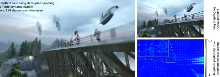
Classical MSAA No Depth of F ield Shader e xc ecutions/pix el with dec oupled sampling 1 27 Depth of Field using Decoupled Sampling

27 visibility samples/pixel avg. 1.67 shader executions/pixel

Fig. 1. Efficient depth-of-field using decoupled sampling in a recent Direct3D game, with 27 visibility samples per-pixel. The heat map encodes the amount

of shading required over the image. Existing supersampling techniques would require 27 shading samples (red) over the entire image, which is prohibitively expensive, while decoupled sampling achieves similar quality with an overall average shading cost of only 1.67 samples per-pixel, similar to current edge multisampling antialiasing (MSAA) with no depth-of-field or motion blur. The visible tile structure in the heatmap is due to the rasterizer scanning pattern.

We present implementations of decoupled sampling that ex-tend two main graphics pipeline architectures: a sort-last fragment pipeline similar to current GPUs and the tile-based sort-middle pipeline of Intel’s Larrabee [Molnar et al. 1994; Eldridge 2001; Seiler et al. 2008]. Our implementation and evaluation focussed on three primary levels of validation:

• A feature-complete functional simulator of Direct3D 9 aug-mented with decoupled sampling and stochastic rasterization to validate the feasibility and resulting image quality of the al-gorithms on real content, and its interaction with the subtleties of a real API.

• Implementation in simulated parallel pipelines to confront ma-jor architectural issues and validate the feasibility and correct-ness of the proposed designs.

• Microbenchmarks, performed on real content with a combina-tion of instrumentacombina-tion and microarchitectural simulacombina-tion in our functional simulator, to isolate and study the effects of the key design choices in our proposed real-world architectures. 2. RELATED WORK

2.1 Antialiasing, Motion Blur and Depth-of-Field

Supersampling.High-quality antialiasing, motion blur, and depth-of-field can be computed by supersampled rendering, e.g. using an accumulation buffer [Haeberli and Akeley 1990] or stochastic rasterization [Cook et al. 1984; Cook 1986; Akenine-M¨oller et al. 2007; Fatahalian et al. 2009]. Accumulation buffer rendering works by rendering samples in time and on the lens as successive render-ing passes. This linearly scales the load across the entire pipeline and is generally too expensive for modern games. Stochastic raster-ization supersamples only the fragment stages (not the per-vertex computation) of the graphics pipeline, saving substantial overhead, but it still scales linearly in fragment shading.

2D Blur Effects.Motion blur and depth-of-field can also be ap-proximated via a family of 2D blur techniques applied directly to a conventional, non-blurred framebuffer [Hammon 2007; Rosado 2007]. These techniques require only a small framebuffer and

per-form well on current hardware, but they suffer from approximations and ambiguity in occlusion. Breaking the scene into layers reduces occlusion artifacts, but cannot eliminate them with modest numbers of layers [Max and Lerner 1985]. Recent layer-based algorithms [Lee et al. 2009] can perform well, but at the cost of substantial al-gorithmic complexity and numerous heuristics. In the limit, making layered rendering fully support occlusion would require a layer per-primitive for shading. In effect this is exactly what decoupled sam-pling does, but on-demand and in a fine-grained fashion within the rendering pipeline, rather than as a series of global passes through memory. To date, accurate stochastic visibility sampling remains the method of choice for production-quality rendering.

2.2 Decoupled Shading and Reuse

Reyes. Decoupled sampling is inspired by Reyes’s separation of shading and visibility rates. However, rather than using microp-olygons, it rasterizes the input geometry directly, and shading is driven by visibility samples, as in conventional graphics hardware. A pipeline similar to Reyes has been implemented on a stream pro-cessor by Owens et al. [2002]. The problem of parallel generation of micropolygons by splitting and dicing has been recently treated by Patney and Owens [2008] and Fisher et al. [2009]. In contrast, we focus on enabling effects that require high visibility sampling rates and on enabling shading reuse in the presence of blur.

Note that, in contrast to a simple framebuffer, Pixar’s Render-Man implementation stores a sorted list of visible micropolygons per sample, which enables order-independent transparency, but re-quires complex, variable-rate storage. We view the problem of order-independent transparency as orthogonal to the shading ar-chitecture and stochastic visibility sampling, and our approach can benefit from similar multilayer framebuffer algorithms.

Lightspeed’s indirect framebuffer eliminates overshading and enables interactive rendering of motion blur, depth of field and transparency for relighting by preprocessing Reyes’ full visibil-ity structure for a fixed scene and viewpoint [Ragan-Kelley et al. 2007]. Shadermaps [Jones et al. 2000] precompute time- and view-independent parts of a shader to save computation over an entire animation.

color blend rasterizer shader

gpu

memory

display

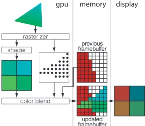
Fig. 2. Multisampled antialiasing in a conventional GPU pipeline.

Edge-tests are computed and visibility is processed (in the framebuffer) at super-sampled resolution, while shading is computed at pixel resolution. The final display is filtered down to pixel resolution from the supersampled frame-buffer.

Multisampling. MSAA can be seen as a specialized instance of decoupled sampling where only subpixel x, y locations are sam-pled [Akeley 1993]. It does not support motion blur, depth-of-field, or flexible shading domains since it requires a static, one-to-n rela-tionship between shading and visibility samples. Motion blur and depth-of-field can cause a one-pixel-sized region of a triangle (a single shading sample) to influence variable numbers of visibility samples, potentially across many pixels.

Caching.A different way of reducing shading cost is to reuse shaded values opportunistically from frame to frame. The Mi-crosoft Talisman architecture [Torborg and Kajiya 1996] sought heavy reuse by using 2D warping to update the full 3D view at a lower frame rate. In contrast, we seek full 3D rendering but save on shading costs. Reprojection caching techniques, including the Reverse Reprojection Cache [Nehab et al. 2007; Sitthi-Amorn et al. 2008] and the approximation cache in Hasselgren’s Multiview Ras-terization Architecture [2006], reuse values from previous frames or views to approximate shading. When a cache miss occurs, they recompute shading in the new view, but do not update the cache for nearby samples to reuse. In decoupled sampling, when a cache miss occurs, a shaded value is computed and the cache index is updated immediately for subsequent samples to reuse. Shading is performed in a single well-defined domain, so results are deterministic regard-less of whether they hit or miss in the cache. This is essential for avoiding artifacts due to discontinuities in the subpixel spacing at which shading was performed (Fig. 4). Decoupled sampling is also robust to occlusion and transparency, because it only reuses shad-ing within a primitive. Further, Talisman and reprojection cachshad-ing store and fetch from the entire previous frame buffer which must be streamed in from texture memory. In contrast, decoupled sam-pling processes all the samples for a triangle together in a single pass and performs memoization dynamically inside the pipeline. In particular, our memoization cache can be small and kept on-chip because it only stores data for the triangles that are in flight. It does not share computed values across frames.

Variable Shading Rates.Yang et al. [2008] apply global level-of-detail per-frame in a general real-time rendering system by ren-dering a subsampled image and using edge-preserving upsampling to the final resolution. Several earlier authors have also described

adaptive subsampling and intelligent upsampling in particular use cases. Direct3D 10.1 can dynamically adapt shading frequency by selecting between per-pixel or per-visibility sample shading in MSAA. Decoupled sampling extends this and adds more flexibil-ity, allowing for shading over arbitrary domains like object space, and for continuous adaptation of the shading rate, where sample correspondences are complex.

3. DECOUPLED SAMPLING

We first describe decoupled sampling in its simplest form, be-fore discussing specific implementations in the context of high-performance parallel pipelines. We define visibility samples as the points which are tested against the triangle edges and the Z-buffer, and shading samples as the points at which surface color is com-puted.

3.1 Algorithm

Decoupled sampling builds on standard rasterization-driven graph-ics pipelines, as shown by the following pseudocode.

1for each triangle

2 setup, compute edge equations 3 for each visibility sample (x, y, u, v, t)

4 if inside triangle AND passes Z// visibility driven

5 map (x,y,u,v,t) to shading index S// decouple domain

6 if S is in memoization cache 7 color ← cache[S]// reuse

8 else

9 color ← compute shading// shade on-demand

10 cache[S] ← color// dynamic cache update

11 framebuffer[x,y,u,v,t] ← color// fully supersampled First, an input triangle is rasterized against visibility samples, which might include extra dimensions for time t and lens uv (line 3-4). We assume an API extended to provide per-vertex motion vec-tors as well as lens aperture size and focusing distance. Decoupled sampling is mostly agnostic to the details of rasterization, and var-ious strategies can be used, as described in our results.

To achieve decoupling, a visibility sample that passes rasteriza-tion and early-Z is mapped into the shading domain of the current triangle (line 5). For example, shading can be performed an ex-pected once per pixel by mapping visbility samples to the same barycentric location at the beginning of the exposure, in the view from the center of the lens, and snapped to the middle of near-est pixel. This provides a many-to-one mapping to a discrete grid, and many visibility samples map to the same shading index. (Sec-tion 3.2 discusses the possible mappings.)

This provides us with a deterministic shading index S, which is tested against a memoization cache (line 6). The value for S might have already been requested by another visibility sample mapping to the same index, in which case we can simply reuse it and avoid recomputation (line 7). If it is not present, we trigger a shading re-quest (line 9), and once the value is computed, we update the cache immediately (line 10). When using a fixed-size cache to approxi-mate memoization, we need to free old values to make room for new ones when the output buffer is full. Our implementations free the least recently used item, where time of use is updated each time the entry is looked up.

Finally, the framebuffer at the visibility sample location is up-dated with the shaded value. Note that the framebuffer is stored at the full supersampled resolution, but might contain the same shaded value multiple times due to reuse in line 7, as in MSAA.

no motion linear motion vectors no motion rotation

Fig. 3. Simple failure cases for our two key approximations: assuming

lin-ear motion over the shutter interval, and shading at a single discrete time and aperture location per-frame. Note the dilation and fuzzy edge of the spin-ning red checkered sphere: with precise motion it should remain round and hard-edged. Similarly, smeared specular highlights on the spinning beach-ball should remain stationary.

For intuition about reuse, one can consider all the visibility sam-ples that share the same shading value: a given shading value gets smeared across the screen according to motion blur or defocus. This is in stark contrast to MSAA, where a shaded value only affects visibility samples within a single pixel. But decoupled sampling is a pull or gather process, where visibility samples request shading values. This is in contrast with micropolygon shading, where col-ors are computed on the surface first, and then scattered into all visibility samples they may touch.

3.2 Decoupling Mapping

Our standard decoupling mapping S simply shades once at the be-ginning (or middle) of the shutter interval, as seen from the cen-ter of the lens. For this, the rascen-terizer provides barycentric coordi-nates defined on the clipspace triangle for each visibility sample. These clipspace barycentrics are used to compute the correspond-ing clipspace position on the t = u = v = 0 triangle, which is then projected onto the screen. We simply discretize the obtained image coordinates to the nearest pixel center. Note that, in the absence of motion and defocus blur, this gives the same result as MSAA. This mapping from clipspace barycentrics to shading coordinates is a simple 2D projection that can be represented by a 3 × 3 matrix.

Degeneracies.The mapping from barycentrics to shading loca-tions needs to be chosen so as to avoid degeneracies. For instance, if the triangle is behind the eye in the beginning of the time interval, its image as seen from lens center at t = 0 is not a valid shading domain. Similar cases include triangles that degenerate to line seg-ments as seen from the lens center. In such cases we choose an alternate mapping. In practice, we use t = 1 if the corresponding triangle is non-degenerate, or directly shade in barycentric space in extreme cases where no single reference view is sufficient, since barycentric space is always well-defined. This can be seen as the 3D/5D equivalent of shading at an alternate sample location if the pixel center is outside the triangle in 2D MSAA. It should be noted that there is no overhead caused by degenerate mapping configu-rations: the decision is made once per triangle, and does not af-fect rasterization, only the projective mapping from barycentrics to shading coordinates.

Approximations.Like Reyes, our technique assumes that shading does not vary much across the aperture and during the exposure. While this is reasonable for many configurations, it has some limi-tations. For instance, highly view-dependent reflections on moving objects are not handled correctly; the highlight due to a station-ary light on a spinning, glossy ball should stay the same over the whole frame (Fig. 3, right). Similar to MSAA, once-per-pixel shad-ing may also yield artifacts for complex non-linear shaders such as bump-mapped specular objects (Fig. 5). Also, per-vertex motion vectors cannot encode curved motion. This is notable for spinning

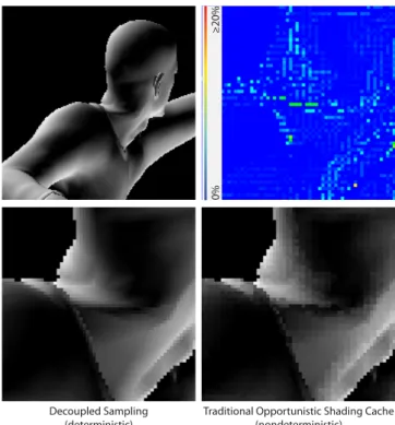
Traditional Opportunistic Shading Cache (nondeterministic) Decoupled Sampling

(deterministic)

0%

≥20%

Fig. 4. Decoupled shading vs. nondeterministic caching (Reprojection

Caching, Multiview Rasterization). Shading at the exact location of a shad-ing cache miss, as done by nondeterministic cachshad-ing schemes, introduces visible errors. Decoupled sampling produces high-quality results by com-puting shading at locations determined by a smooth deterministic mapping from visibility samples to a well-defined shading grid. Meanwhile, oppor-tunistic caching results in an unpredictable and non-smooth mapping of shading samples into screen space, producing shading discontinuities. objects (Fig. 3, left). However, this limitation is orthogonal to de-coupled sampling, and it can be addressed either by adding time as a dimension in the decoupling mapping and shading cache in-dices (so that the shading domain becomes a 3D volume), or like RenderMan by combining decoupled sampling with accumulation buffering.

3.3 Extensions

Bilinear Reconstruction.So far we have defined the cache lookup as a nearest-neighbor filter: visibility samples take the value of the closest corresponding shading location. We also support bilinear reconstruction. If the shading domain is 2D (e.g. pixel grid at t = 0 in the center view of the lens), we simply interpolate between the four closest shading locations. Note that this means that a cache miss in line 8 of the pseudocode now triggers the computation of four values.1 _{This can be easily generalized to a shading domain}

of higher dimensions, for instance trilinear lookups with shading values varying in both space and time. (See the figure in supple-mentary material for an example.)

Controllable shading rate. The mapping between visibility sam-ples and shading locations can be adjusted by the programmer on a per-primitive or per-shader basis. In particular, it can be desirable to adjust the shading rate according to the spatial complexity of a shader: a matte shader can be sampled only once per pixel, but a

1_{Note that in practice samples are shaded in quadruplets anyway because}

4 visibility samples

1 shading sample 64 visibility samples1 shading sample

4 visibility samples

4 shading samples 64 visibility samples16 shading samples

Fig. 5. An illustration of controllable shading rate in the case of an

alias-ing bump map. Top row: At only 1 shadalias-ing sample per pixel, visibility sam-pling rate has no effect on the aliasing. Bottom row: Increasing the shading sampling rate alleviates aliasing problems. The shading can be supersam-pled at its own frequency independent of visibility. The shading rate can be controlled per-primitive or per-shader.

shiny surface with high-frequency bump mapping can require shad-ing computation at full supersampled resolution to reduce aliasshad-ing (Fig. 5). Decoupled sampling supports controllable shading rate by simply modifying the mapping function S in line 5, allowing smooth and continuous control of shading granularity.

Adaptive shading rate. Shading rate can also be adapted auto-matically based on the configuration of the current primitive or ob-ject. In the context of depth of field, we have experimented with a shading rate that depends on defocus blur such that the interval between shading samples is proportional to the circle of confusion. The circle is computed conservatively at the vertices such that the minimum blur dictates the shading rate for the whole primitive. When the whole triangle is out of focus, the shading grid is coarser than the pixel grid. Combined with bilinear reconstruction, this can yield significant savings at little impact on the image. The image in Fig. 6) was computed at little error at an average of 1.3 shader invo-cations per pixel using adaptive shading grid resolution, compared to the average shading rate of 2.05 when using a fixed 1:1 mapping. Note that alpha-tested primitives cannot be effectively subsampled because the shading affects visibility.

3.4 Discussion

Decoupled sampling is visibility driven: shading values are com-puted only when requested by a visible visibility sample. This is in contrast to Reyes, where micropolygons are shaded before rasteri-zation, with only conservative knowledge of visibility.

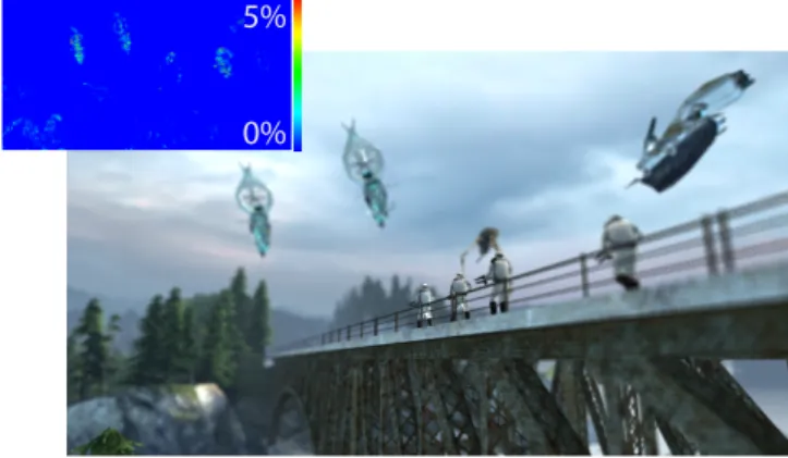
5%

0%

Fig. 6. This image from Half-Life 2 Episode 2 was rendered with 27

vis-ibility samples per pixel using adaptive shader subsampling and bilinear reconstruction from a 256-quad shading cache. The shading rate was an av-erage 1.3 times per pixel. The error plot shows relative image difference to the same frame rendered using non-adaptive 1:1 mapping of screen pixels to shading locations, which had an average shading rate of 2.05 per pixel.

In contrast to opportunistic schemes that seek to reuse shad-ing across primitives and frames, we reuse shadshad-ing samples only within a single primitive during a single frame. This makes our ap-proach robust to occlusion and transparency, because other primi-tives cannot occlude or change cache entries due to blending. While the shading domain might be aligned with the screen, the cache is independent of the framebuffer. In particular, exactly the same shaded values are returned for a given visibility sample irrespective of whether it was cached or recomputed, making the shading en-tirely deterministic and independent of computation order (Fig. 4). Furthermore, the freshly computed shading values are placed into the cache immediately for fine-grained reuse without having to wait for the next frame.

The mapping used for computing the shading index S for a given x, y, u, v, t tuple is a free parameter in our method, enabling us to super- or subsample shading spatially (Fig. 6), or even easily add more dimensions like time-dependency when necessary.

Shading generally requires derivatives for antialiasing, e.g., mip-mapping. We enable this by shading quadruplets of shading sam-ples at a time, similar to current GPUs. We incur similar overshad-ing at boundaries, and also need to “snap” shadovershad-ing locations of samples that fall out of the triangle to ensure valid interpolation.

Because memoized shading results stand in for actual shader ex-ecution, any secondary results of the shader invocation must also be retained. In particular, pixel and alpha kill/discard results must be memoized and applied to all visibility samples that use the same shading sample. Similarly, all render target outputs must be mem-oized together.

4. GRAPHICS PIPELINE IMPLEMENTATIONS

Decoupled sampling was designed with modern real-time graph-ics pipelines in mind, meant to be an evolutionary change which retains existing optimizations where possible. We explore the im-plementation of decoupled sampling in two main graphics pipeline architectures: a sort-last fragment pipeline similar to current hard-ware GPUs, and Larrabee’s tile-based sort-middle pipeline [Molnar et al. 1994; Eldridge 2001; Seiler et al. 2008].

Decoupled sampling is implemented by augmenting these pipelines with 1) a space-time-lens rasterizer that computes the barycentrics of all visibility samples, using stochastic sampling for lens and time, 2) decoupling logic that defines the mapping from barycentrics to shading space and the hash to the shading indices, 3) a shading cache for memoization of shading samples, generally stored on-chip and local to the shading system or fragment back-end, and 4) cache management logic that manages reference count-ing and shader completion trackcount-ing, as well as the replacement pol-icy.

The primary concerns in real-time graphics systems are paral-lelism and the memory hierarchy. Multithreading is used to hide long memory latencies and maintain high ALU utilization, but re-quires coherent behavior, as well as on-chip memory to maintain state (registers) for the many parallel items in flight. Processing order, driven by the synchronization points (middle and sort-last), determines memory access patterns and cacheability. Finally, sorting and distributing parallel items at synchronization points re-quires memory—either on-chip or off—for buffering. These archi-tectural themes underly our design considerations, and distinguish the tradeoffs and relative cost of different implementations in the two styles of pipeline we studied.

4.1 Efficient Implementation

Costs.We first consider the basic costs of adding decoupled sam-pling. An efficient real-time hardware implementation needs on-chip memory to cache memoized shading values for quick reuse. In many cases it is possible to reuse existing buffer points for caching, but larger reuse windows might create pressure to make them bigger. Motion blur and depth of field may also impact the efficiency of color and depth compression, though earlier investiga-tions have shown that some existing compression schemes can still perform reasonably [Akenine-M¨oller et al. 2007]. In addition, there are modest arithmetic costs for tracking barycentrics for visibility samples, mapping and hashing them to shading samples, and per-forming cache lookups and management. These per-sample costs are small compared to shading per-visibility sample, but can still grow significant as sampling rate increases.

Visibility & Shading Coherence. High performance graphics pipelines drive fragment processing using screen-space 2D block traversals optimized to maintain coherence simultaneously in visi-bility computation, shading and texture access, and framebuffer up-dates. By remaining visibility driven, decoupled sampling retains visibility coherence optimizations, but because it decouples shad-ing from visibility samplshad-ing, shadshad-ing coherence is no longer ex-plicitly guaranteed – motion blur and depth of field cause the same shading samples to touch many pixels. However, our experiments (Section 5.3) indicate that a standard space-filling 2D traversal is sufficient to maintain coherence in the shading cache, and in par-ticular to avoid pathological behavior. The reuse rate is influenced both by size of the cache, and somewhat by the amount of motion and defocus blur (Fig. 9).

While the basic decoupled sampling algorithm logically shades individual shading samples, our implementations compute and cache shading in blocks in shading space to enable coherent SIMD execution, exactly as in a non-decoupled pipeline: the shading en-gine is not altered, and intra-block coherence is identical. In par-ticular, the shading request batch size can be used for trading off potential overshading for greater shading coherence similar to ex-isting GPUs.

Texture Coherence.While texture coherence is unaltered within shading blocks, the order in which these blocks are issued can be

altered by decoupling. However, this effect is local: since triangles are rasterized in-order and do not share shading samples, reorder-ing due to blur and shadreorder-ing cache misses may only occur within the shading blocks generated by a single triangle. The modern dy-namic thread schedulers that drive shaders (hardware schedulers in traditional GPUs and software fiber switching in Larrabee) are already designed to tolerate large fine-grained variation in texture latency due to unpredictable misses. Our experiments confirm that texture caching and bandwidth are largely unaffected by decoupled sampling (Section 5.3).

4.2 Cache Management & Synchronization

To implement our cache in a modern pipeline with multiple asyn-chronous and parallel stages and multiple triangles in-flight at once, the shading cache indices are augmented with triangle IDs. The re-sulting unique cache indices are used for tracking the cache entries throughout their lifetime. Shaded colors are not consumed until the backend of the pipeline, and thus cache entries cannot be freed until all outstanding references to them are fulfilled. Outstanding refer-ences are tracked using simple reference counting. This is similar to a conventional sort-last GPU pipeline, except that buffer entries may be referenced by more than one fragment’s visibility samples, so their reference count must be more than 1 bit. In addition, in pipelines where shaders can complete out-of-order and indepen-dently from framebuffer processing (like sort-last GPUs), an addi-tional flag is needed to track whether a shading block has completed and its results populated in the cache before it is used by the back-end. Finally, when the output buffer is full, an old value is freed to make room for a new one. Our implementation frees the least re-cently used non-outstanding item. This is enforced conservatively: when the cache is full with entries that have not been consumed, new shading requests stall.

4.3 Sort-Last Fragment

Modern GPUs primarily use variants of the sort-last fragment ar-chitecture (Fig. 7) for synchronization and enforcing in-order ex-ecution: shaders execute in parallel, independent from pixel pro-cessing, and complete out-of-order. Strict ordering is enforced us-ing reorder buffers of hundreds or thousands of entries before the raster operation (ROP) units that update the framebuffer. This al-lows fragments to be kept asynchronous and independent to as late as possible in the pipeline, maximizing available parallelism at the cost of fine-grained global synchronization.

We propose to reuse the existing reorder buffer between the shad-ing and framebuffer stages as an explicit cache (Fig. 7, bottom left). In a standard pipeline, output slots are allocated for every block of shading samples as it is sent to the shader, and they are freed as soon as they are consumed by the framebuffer update. When the reorder buffer is full, earlier stages of the pipeline stall.

For decoupled sampling, we similarly allocate storage for shaded colors when new shading samples are issued. To leverage reuse, we do not free values as soon as they are first consumed, but rather leave them in the buffer to be potentially reused by future visibility samples. When an already-present shading sample is requested, we only emit the corresponding cache indices into the output buffer, and reference count the corresponding buffer entries. This intro-duces two new architectural pressures. First, higher reuse rates call for extending the lifetime of items, implying an increase the buffer size. (We study the effect of cache size on shading reuse in Sec. 5.) Second, the reorder buffer may require more fine-grained read ports

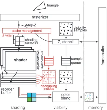
shader rasterizer Z, stencil color blend fr ameb uf fer 3 1 5 2 2 4 3 ₁ 2 3 1

shading visibility memory

triangle visibility samples decoupling indices if miss: shading samples cache management reorder buffer sample queue early-Z sync hr onous as ync hr onous

Fig. 7. A modern sort-last GPU fragment pipeline, augmented with

de-coupled sampling. Modifications required for dede-coupled sampling are high-lighted in red.

to support efficient reads from more than one shading sample block per block of visibility samples. In general, though, decoupled sam-pling is a natural fit in a modern sort-last pipeline, since shading and visibility processing are already “decoupled” by asynchronous execution.

We validated our design for synchronization and resource man-agement by building a transaction-level simulator of a modern, par-allel GPU fragment pipeline modeled after ATI R6xx and extended with decoupled sampling. The greatest practical architectural pres-sure is the high framebuffer bandwidth incurred by high supersam-pling rates required by depth of field and motion blur. This issue is orthogonal to decoupled sampling, but we studied it to understand its role in the overall cost of motion blur and depth of field (Fig. 11). Discussion.A sort-last implementation of decoupled sampling naturally allows a single, global shading cache. This leads to max-imal shading reuse for a given raster traversal order and shading cache size, because coherence is not lost due to tiling. Such max-imal reuse is achieved at the cost of having to support concurrent access from large numbers of threads through many fine-grained cache read ports. However, as shader outputs need to be buffered and globally reordered even without decoupling, other architectural changes are small. Because memoization is implemented by allow-ing items to remain buffered past their first use, the only effect of caching is extending the lifetime of entries past when they are first completed and consumed by the color buffer. In this context, the ef-fective cache size overhead relative to a non-decoupled pipeline is those items that would have been retired after first reference but are kept for re-referencing. If the framebuffer processing is strictly in-order, this overhead is limited by the size of the triangle currently being drained through the ROPs, even if many more are in-flight after it, because their shading samples could not have been freed from the buffer even without decoupling.

4.4 Tile-Based Sort-Middle

In a tiling-based rendering architecture, a front-end pass trans-forms primitives, computes their coverage, and enqueues them at the screen tiles they overlap. A separate back-end pass processes all pixels in each tile, shading them and blending them into the framebuffer. By front-loading a screen-space sort of the geome-try, they globally synchronize over triangles rather than pixels, and thereby dramatically simplify concurrency in fragment and pixel processing. Within a single pixel2_{, all processing is synchronous}

and strictly in-order over the lifetime of a rendering pass all the way into the framebuffer. This execution model fundamentally cou-plesshading and visibility samples by tying together shading with framebuffer processing, so it does not require synchronization, re-ordering or explicit inter-stage buffering in the back-end. The trade-off for the simplicity of coarse-grained global synchronization is that triangles may cover multiple tiles, requiring redundant stor-age and processing. Any per-triangle backend computation (raster, interpolant construction, etc.) is potentially duplicated, as is tile queue storage (termed bin spread by Seiler et al. [2008]), and visi-bility and shading coherence is lost across tile boundaries because of asynchrony between the tiles.

These design tradeoffs are potentially challenging for decoupled sampling. Losing coherence across tiles reduces the effectiveness of shading reuse, and any storage used by the shading cache com-petes with the framebuffer in the on-chip memory. This is exac-erbated by blur, which increases bin spread: higher visibility sam-pling rates require more storage per pixel, reducing the screen area covered by a tile in a fixed storage size, and motion and defocus blur increase the screen extents of a triangle, and therefore the number of tiles into which it falls. (We study these effects on bin spread in Section 5.3.3.) Finally, the coupled execution of shad-ing and framebuffer (visibility) processshad-ing is most efficient with a predictable, fixed relationship between shading and visibility sam-ples, where decoupled sampling creates (and exploits) a dynami-cally variable relationship to reduce shading work.

A first strategy to implement decoupled sampling is to simply ex-tend the back-end so that each visibility sample references a unique shading sample, and the prefix the backend processing of each pixel with a cache lookup (and update in case of a miss). However, the ir-regular and variable rate relationship between visibility and shading samples causes a significant shading load imbalance because fixed-size chunks of visibility samples require radically different amounts of shading work. This variable rate relationship also causes poor SIMD utilization, because the whole SIMD batch of visibility sam-ples needs to wait for shading completion in the case of even a sin-gle shading cache miss. In a SIMD architecture, this is equivalent to overshading due to shading an entire block whenever a single sample misses in the cache.

An alternative is to split the back-end into two separate asyn-chronous phases, much like the sort-last fragment pipeline: a shad-ing phase that computes shadshad-ing asynchronously from framebuffer updates, and a ROP phase that performs in-order framebuffer up-dates. This better mirrors the two natural computation domains of decoupled sampling. A basic sort-middle tiling is still performed first, and cores still perform back-end processing in a single pass. Within that pass, however, worker threads that previously only per-formed coupled shading-ROP tasks now dynamically schedule

be-2_{“Pixels” here is a simplification: synchronization is actually over}

frame-buffer samples—output locations—so neighboring triangles covering adja-cent but non-overlapping samples within a pixel may proceed concurrently, since they do not affect the same parts of the framebuffer.

tween shading and framebuffer updates, in effect introducing a per-tile sort-last stage to the pipeline. Just like in a sort-last implemen-tation, buffering is used to queue ROP work which is blocked on shading results, and to reorder shading samples as they complete. This architecture is more amenable to decoupling, and avoids effec-tive overshade due to load imbalance between pixels in a tile, but at the cost of scheduling and buffering for two separate backend stages rather than one. In general, any implementation of decou-pled sampling adds more relative memory overhead to a pipeline with synchronous fragment shading and pixel processing than one which already buffers between the two, like sort-last pipelines.

Discussion.There are several alternatives for implementing the shading cache in a sort-middle architecture. While local, per-tile caches are the simplest, it would be also possible to implement a global shading cache accessed by all tiles concurrently. This is at odds with the sort-middle design goal of reducing global syn-chronization, and the lack of coherence across tiles—the parts of the same triangle that fall into neighboring tiles may be processed far apart in time—makes this approach less attractive. However, this tradeoff could be different for a hardware-schedule sort-middle pipeline, which can more easily afford fine-grained global synchro-nization than a software pipeline like Larrabee. Still, the long-term trends towards ever-greater parallelism will always favor less syn-chronization. In our evaluation (Sec. 5), we focus on comparing a sort-last architecture with a global cache to a sort-middle architec-ture in the limit, with purely local caches and no inter-tile commu-nication.

5. IMPLEMENTATION AND RESULTS

To study Decoupled Sampling, including API integration and other details and interactions, we implemented it in a complete Direct3D 9 functional simulator, extended with APIs to control blur and shad-ing rate. We evaluate decoupled samplshad-ing on actual Direct3D ap-plications running real shaders, including Half-Life 2, Episode 2 and Team Fortress 2, extended to include motion blur and depth of field. We study the architectural implications (cache and shad-ing coherence, framebuffer bandwidth, etc.) on these scenes and describe results in Section 5.3.

5.1 Rasterizer Implementation

The rasterizer enumerates the visibility samples that a given input triangle hits, and computes barycentric coordinates which are sub-sequently mapped into shading indices. While we here describe a particular implementation, the choice of rasterization algorithm is orthogonal to the rest of the decoupling pipeline.

Sampling Patterns.To enable motion blur and depth of field, we rasterize triangle that vary over time and with samples that cover the lens aperture. The samples in our framebuffer have five dimen-sions: two for the subpixel x and y coordinates, and in addition, u, v for lens location and t for time. Like current GPUs, we employ the same x, y sampling pattern for all pixels, but employ stochastic ras-terization and sample lens and time using 3D jittered grid sampling patterns that repeat every 32 × 32 pixels. (Accumulation buffering shares the lens and time pattern across all pixels, which results in highly disturbing aliasing artifacts – see Figure 8, left).

Hit Testing and Edge Functions.We dynamically classify each triangle into moving/non-moving and blurring/non-blurring due to depth of field, and handle each of the four cases by a spe-cialized algorithm. Stationary, non-defocus-blurred triangles are rasterized using an unchanged 2D hierarchical rasterizer. For tri-angles that move, but do not exhibit defocus blur, we employ

time-continuous 3D homogenous edge functions as proposed by Akenine-M¨oller et al. [2007]. For handling stationary triangles that undergo defocus blur, we introduce novel aperture-continuous 4D edge functions. Analogously to time-continuous edge functions, they simplify the per-sample visibility test by pushing common computations out into the triangle setup. See Appendix A for de-tails. In the fully general case of both motion and defocus blurred triangles, we compute the warped triangle that corresponds to the u, v, t of the sample and test for a hit directly, because this turns out to be more efficient than using 5D time-aperture-continuous edge functions.

Scanning Order.We rasterize the triangles by looping over pix-els in the 2D screen bounding box of the triangle, computed as the union of all possible time/lens projections. The screen is scanned in tiles of 32 × 32 pixels, which are processed in a Z curve order. Inside the tiles, individual quadruplets of pixels are also rasterized along a Z curve. To avoid the cost of testing each sample in the entire bounding rectangle, we utilize sub-rectangles defined by the strata of our sampling pattern in a way similar to Pixar’s Render-Man implementation, and also analyzed by Fatahalian et al. [2009] for micropolygons.

Motion blur and depth-of-field can alter the efficiency of dif-ferent sample layouts and raster stamp traversal orders. We fol-low traditional multisampling GPUs and densely store all subpixel samples for a given pixel together in the same block. This corre-sponds to blocks which are narrow in x, y but span the full u, v, t range. Motion blur and depth of field may also impact the efficiency of color and depth compression. While earlier investigations have shown that some existing compression schemes may still perform reasonably [Akenine-M¨oller et al. 2007], we view further evalu-ation of both memory layouts and compression as orthogonal to decoupled sampling and leave it as future work. All of our results assume no framebuffer compression.

5.2 Qualitative Results

To compare image fidelity to accumulation buffering and full stochastic supersampling with varying sampling rates, we present results for an application featuring local deformable precomputed radiance transfer (Fig. 8) [Sloan et al. 2005]. Decoupled sampling (center) is compared to accumulation buffering (left) and stochastic supersampling—both of which shade every visibility sample—and observe shading quality similar to full stochastic supersampling at only a fraction of the shading cost. The supplementary material contains a video showing the scene in motion, including motion blur and a focus rack, rendered using different numbers of visibil-ity samples and the comparison algorithms.

5.3 Evaluation

We studied the effects of the additional computational and memory requirements related to decoupled sampling, supersampled visibil-ity, and motion blur and depth of field by instrumenting our Di-rect3D 9 functional simulator. We gathered statistics on shading, texture, and framebuffer coherence as a function of sampling rate, amount of defocus/motion blur, and shading cache size for both tiled and non-tiled architectures. The amount of blur or blur area is reported as the average number of pixels a single shading sample touches. This is equivalent to the average circle of confusion for scenes with just depth of field, and the length of the motion trails for pure motion blur (assuming a 1-pixel wide path). The measure-ments are shown in Figure 9 and analyzed below.

Accumulation buffering Decoupled Sampling Stochastic Supersampling 8 Visibilir y S amples per P ix el 64 Visibilit y S amples per P ix el 27 Visibilit y S amples per P ix el

Shading rate: 4-11 Shading rate: 64

Shading rate: 64

Shading rate: 4-7 Shading rate: 27

Shading rate: 27

Shading rate: 3-5 Shading rate: 8

Shading rate: 8

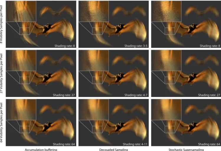
Fig. 8. A comparison of accumulation buffering, decoupled sampling, and stochastic supersampling. Top to bottom: 8/27/64 samples/pixel. Decoupled

sampling (center) attains image quality similar to full stochastic supersampling (right) with only a small fraction of the shading cost. Accumulation buffering (left) shows significant banding and strobing artifacts, despite shading just as much as stochastic supersampling.

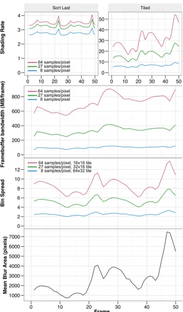
5.3.1 Shading Coherence. Figure 9 analyzes the effectiveness of the shading cache in capturing reuse for different sizes of cache and amounts of defocus and motion blur for two test scenes for both global (sort-last) and tiled (sort-middle) implementations of decoupled sampling. The Half-Life 2, Episode 2 scene (left col-umn) exhibits defocus blur and the Team Fortress 2 scene (right column) exhibits motion blur due to camera egomotion. Figure 12 similarly analyzes shading cache coherence over 50 frames of ani-mation with simultaneous depth of field and object motion blur for the scene in Figure 8.

With a global (sort-last) shading cache, shading rate stays nearly constant as a function of blur area and sampling rate, varying over at most a 3x range from 8 samples/pixel with no blur to the most in-coherent blur at 64 samples/pixel in the same scene (Fig. 9, right). This is the goal of decoupled sampling, and it is extremely suc-cessful. The game frames do exhibit some variation in shading rate as a function of blur, likely because they both include large, heav-ily blurred background polygons which are much larger than any reasonable shading cache. The animated bats (Fig. 12 and accom-panying video), meanwhile, contain only small triangles and shad-ing rate exhibits virtually no variation (less than 20%) over an even wider variation in blur area.

In a sort-middle implementation, local shading caches per-tile reduce potential shading reuse, because shading is not shared across tile boundaries. Our simulation assumes no sharing between screen-space tiles, which represents the worst-case behavior of the most extreme tiled renderer design. Indeed, the shading rate plateaus at a rather low reuse rate due to lost shading coherence. With tiling, shading rate grows much more as a function of blur, since blur increases bin spread. The slope of shading rate growth as a function of blur is steeper at higher sampling rates, since they reduce effective tile size. However, even losing substantial shading reuse due to tiling, decoupled sampling still shades significantly fewer samples than supersampling. To emphasize this, the second row of graphs shows the same data, but graphed as savings (higher is better) compared to an idealized supersampling implementation which shades exactly once per visibility sample. Even at high lev-els of blur, though less effective than a global cache, the decou-pled tiled renderer still shades 2-12x less than supersampling in the game frames, with reasonably sized caches. The bats animation, with even higher blur and substantial overshade on small polygon boundaries (giving an ideal shading rate above 3), however, strug-gles to shade much less than an idealized supersampling engine

Heavy

blur Moderate blur No blur Moderate

blur No blur Heavy blur

0 1 2 3 4 5 Sort Last ●●● ● ● ● ● ● ● ● ● ● ● ●●● ● ● ● ● ● ● ● ● ● ● ●●● ● ● ● ● ● ● ● ● ● ● 0 50 100 150 200 250 Tiled ●●● ● ● ● ● ● ● ● ● ● ● ● ●●● ● ● ● ● ● ● ● ● ● ● ●● ● ● ● ● ● ● ● ● ● ● 0 50 100 150 200 250 0 5 10 15 Sort Last ● ● ● ● ● ● ● ● ● ● ● ● ● ● ● ● ● ● ● ● ● ● ● ● ● ● ● ● ● ● 0 20 40 60 80 100 120 Tiled ● ● ● ● ● ● ● ● ● ● ● ● ● ● ● ● ● ● ● ● ● ● ● ● ● ● ● ● ● ● 0 20 40 60 80 100 120

Samples shaded / pixel Samples shaded / pixel

Mean blur are (pixels) Mean blur area (pixels) Mean blur area (pixels) Mean blur area (pixels)

64 samples/pixel 27 samples/pixel 8 samples/pixel

Moderate blur Moderate blur

Moderate blur Moderate blur better better 64 samples/pixel 27 samples/pixel 8 samples/pixel 0 10 20 30 40 Sort Last ●●● ● ● ● ● ● ● ● ● ● ● ● ●● ● ● ● ● ● ● ● ● ● ● ● ●● ● ● ● ● ● ● ● ● ● ● 0 50 100 150 200 250 Tiled ● ●● ● ● ● ● ● ● ● ● ● ● ● ●● ● ● ● ● ● ● ● ● ● ● ● ●● ● ● ● ● ● ● ● ● ● ● 0 50 100 150 200 250 0 10 20 30 40 Sort Last ● ● ● ● ● ● ● ● ● ● ● ● ● ● ● ● ● ● ● ● ● ● ● ● ● ● ● ● ● ● 0 20 40 60 80 100 120 Tiled ● ● ● ● ● ● ● ● ● ● ● ● ● ● ● ● ● ● ● ● ● ● ● ● ● ● ● ● ● ● 0 20 40 60 80 100 120 Shading savings vs. supersampling _{Mean blur area (pixels) Mean blur area (pixels)} Shading savings vs. supersampling _{Mean blur area (pixels) Mean blur area (pixels)}

Moderate blur

Moderate blur Moderate blur

Moderate blur better better 64 samples/pixel 27 samples/pixel 8 samples/pixel 64 samples/pixel 27 samples/pixel 8 samples/pixel 0 10 20 30 40 Sort Last 24 ₂6 ₂8 ₂10 ₂12 ₂14 Tiled 24 ₂6 ₂8 ₂10 ₂12 ₂14 0 10 20 30 40 Sort Last 24 ₂6 ₂8 ₂10 ₂12 ₂14 Tiled 24 ₂6 ₂8 ₂10 ₂12 ₂14

Shading savings vs. supersampling

Shading savings vs. supersampling 16 64 256 1k 4k 16k16 64 256 1k 4k 16k_{Shading cache size (samples) Shading cache size (samples)} 16 64 256 1k 4k 16k_{Shading cache size (samples) Shading cache size (samples)}16 64 256 1k 4k 16k

break-even break-even break-even break-even

better better 64 samples/pixel 27 samples/pixel 8 samples/pixel 64 samples/pixel 27 samples/pixel 8 samples/pixel Team Fortress 2 Half-Life 2, Episode 2

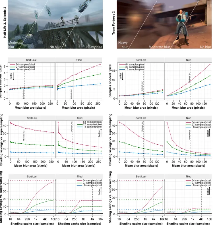
Fig. 9. Shading work for global sort-last and purely local tiled implementations of decoupled sampling, as a function of blur and shading cache size, at 8, 27

and 64 visibility samples per pixel. Shading rate (row 1) is the average number of shader invocations per pixel of coverage (lower is better). Shading savings gives the factor of reduction in shading work relative to an idealized supersampling implementation which shaded exactly one sample per visibility sample. The dotted lines in the shading cache size graphs (row 3) show the ideal shading savings using an infinite-sized cache. The top 2 rows use a 4k-sample shading buffer. The amount of blur is reported as the average area (in pixels) touched by a single shading sample. The horizontal axis ranges from no blur on the left to severe blur on the right (illustrated in the top row images). The moderate blur setting corresponds to all renderings seen elsewhere in the paper.

with tiled caches, while a global cache still performs nearly per-fectly.

Motion blur (Fig. 9, right) leads to greater shading incoherence than defocus blur (Fig. 9, left) per unit of blur area. This is caused by interaction with the 2D space-filling rasterization traversal or-der: defocus blur is confined to a compact area on this space-filling traversal, while motion blur causes longer streaks, spanning a wider range of the traversal for the same number of pixels touched. De-pendence on the raster traversal order also implies that motion di-rection may affect shading coherence. We ran tests with synthetic (uniform) motion blur to study the effect of motion direction, and observed a ±20% variation over a 360◦ _{rotation, suggesting that}

a standard space-filling order effectively mitigates pathological be-havior.

The last row of graphs in Figure 9 depicts the savings obtained as a function of cache size, at a fixed, moderate level of blur (cor-responding to the images rendered elsewhere throughout the pa-per, and indicated by the vertical lines in the two graphs above), in comparison to an idealized supersampling renderer that shades exactly once per visibility sample and does not suffer from over-shading at triangle boundaries. Decoupled sampling with quad-granularity shading blocks begins to outperform idealized super-sampling (shading exactly once per visibility sample) when the cache size reaches 128 shading samples. Increasing cache size con-tinues to improve shading performance, especially for scenes with blurry, large triangles (the game frames), up to thousands of sam-ples for a global cache. A 4k-entry (16 kB, for 4 bytes/sample color) global cache provides large benefits (4-35x for the test scenes) for a cost that seems feasible at the time of writing. Conservative per-tile cache performance plateaus at a substantially lower cache size and shading savings than the global cache.

5.3.2 Texture Coherence. While we maintain SIMD ALU co-herence in shaders by shading multiple quadruplets of samples at a time like a normal graphics pipeline, texture locality between blocks might be affected by the on-demand ordering of shader in-vocations and the introduction of blur. We studied this in our Di-rect3D 9 pipeline with a 32kB 16-way set associative texture cache with 64-byte lines, closely modeled after actual hardware. In the Half-Life and Team Fortress frames, we observed per-texel hit rates around 99.6% for non-blurred MSAA images at 8 samples/pixel, and hit rates of over 99.7% for the defocus and motion blurred im-ages using decoupled sampling for all visibility sampling rates. The hit rate is slightly higher with decoupling because a modestly in-creased shading rate generates more references to roughly the same texels. Despite the higher hit rates, texture bandwidth requirements are slightly larger than for the pinhole image (an additional 5-15%, depending on the sampling rate) because more total samples are shaded. Hit rates only deteriorate for  8kB caches, and are no worse than for single sampling. We conclude that the texture cache effects of decoupled ordering are negligible, and that texture cache performance is unaltered by decoupled sampling.

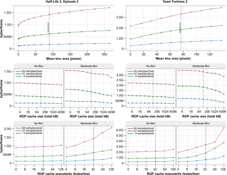
5.3.3 Visibility Coherence. To build a more holistic picture of the broader architectural impact of motion and defocus blur, we in-vestigated the changes in visibility bandwidth—framebuffer band-width and ROP cache coherence for sort-last, and binning data for sort-middle—caused by the blur. (Decoupled sampling is in itself orthogonal to the question, as it only supplies the values read from and written to the framebuffer.)

Bin Spread (Sort-Middle) As discussed in Section 4.4, blur and higher visibility sampling rates affect “bin spread,” the number of screen tiles a primitive touches, in several ways. We studied the

ef-0 2 4 6 8 10 12 ● ● ● ● ● ● ● ● ● ● ● ● ● ● ● ● ● ● ● ● ● ● ● ● ● ● ● ● ● ● 0 20 40 60 80 100 120 0 1 2 3 4 ●●● ●●● ● ● ● ● ● ● ● ●●● ●● ● ● ● ● ● ● ● ● ●● ● ● ● ● ● ● ● ● ● ● ● 0 50 100 150 200 250

Mean blur area (pixels) Mean blur area (pixels)

Bin Spread Bin Spread

Half-Life 2, Episode 2 Team Fortress 2

64 samples/pixel, 16x16 tile 27 samples/pixel, 32x16 tile 8 samples/pixel, 64x32 tile

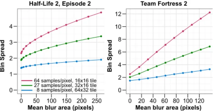
Fig. 10. Bin spread for a tiled architecture as a function of mean blur

size and visibility sampling rate. Large blurs increase the number of tiles touched by a single primitive, while higher sampling rates reduce the x, y tile dimensions which fit in a given fixed-size memory. (This simulation assumes tiles are bounded to at most 128kB.)

fects on our game data assuming tile memories of at most 128 kB. This means tiles get smaller as sampling rates increase, and we ex-pect steeper slopes for bin spread as a function of blur for higher sampling rates. Figures 10 & 12 show bin spread as a function of defocus and motion blur. Defocus blur (HL2, left) causes less dra-matic bin spread increases than linear motion blur (TF2, right). This is again explained by the fact that linear motion paths of similar to-tal screen area are much longer than the lens blur. We conclude that added memory pressure caused by high sampling rates, combined with the effective increase in triangle size caused by blur, make strong motion blur difficult to achieve without an increase in tile memory size. However, moderate amounts of defocus blur seem achievable with an acceptable performance penalty, especially at lower sampling rates.

Framebuffer Bandwidth (Sort-Last) Sort-last pipelines stream over the framebuffer in primitive order. In this context, the main function of a ROP cache is not to allow reuse between primitives updating the same samples, but to coalesce reads and writes for a number of nearby covered samples into larger block transactions. The key question, then, is what impact blur has on the ability to coalesce streaming framebuffer accesses.

We studied ROP cache performance in our three test scenes by measuring the amount of off-chip framebuffer bandwidth in three scenarios: 1) as a function of blurriness with a fixed-size cache, 2) as a function of ROP cache size in a moderately blurred frame, and 3) as a function of cache line size with a moderately blurred image and a fixed-size cache. In our simulation, the framebuffer is laid out along the same Z curve used for rasterizer traversal (Sec. 5.1). The results are presented in Figure 11 & 12. As expected, for a fixed cache and line size (of 128kB and 32 bytes, respectively), we observe increases in bandwidth requirements with larger defocus and motion blurs. However, the increases remain within 50% over MSAA (no blur) even in the case of severe defocus and motion blurs: In short, coalescing still works with motion blur and depth of field. Blur does not increase the total number of samples being tested and updated, it simply spreads them out in space. Neighbor-ing regions of the same surface, however, are likely to sparsely fill in other samples within roughly the same space at roughly the same time, and traditional caches are sufficient to capture this aggre-gate coherence in framebuffer access, both with and without blur. Increasing cache size corresponds to enlarging the window over which samples may be coalesced, while reducing line size

corre-0 500 1000 1500 2000 No Blur ● ● ● ● ● ● ● ● ● ● ● ● ● ● ● ● ● ● 22 ₂3 ₂4 ₂5 ₂6 ₂7 Moderate Blur ● ● ● ● ● ● ● ● ● ● ● ● ● ● ● ● ● ● 22 ₂3 ₂4 ₂5 ₂6 ₂7 0 1000 2000 3000 4000 5000 6000 No Blur ● ● ● ● ● ● ● ● ● ● ● ● ● ● ● ● ● ● 22 ₂3 ₂4 ₂5 ₂6 ₂7 Moderate Blur ● ● ● ● ● ● ● ● ● ● ● ● ● ● ● ● ● ● 22 ₂3 ₂4 ₂5 ₂6 ₂7 1.5G 2.0G 500M 1.0G 5.0G 6.0G 1.0G 4.0G 3.0G 2.0G 4 8 16 32 64 128 4 8 16 32 64 128 4 8 16 32 64 128 4 8 16 32 64 128

ROP cache granularity (bytes/line) ROP cache granularity (bytes/line)

0 500 1000 1500 2000 2500 3000 No Blur ● ● ● ● ● ● ● ● ● ● ● ● ● ● ● ● ● ● ● ● ● ● ● ● ● ● ● ● ● ● ● ● ● ● ● ● 22 ₂4 ₂6 ₂8 ₂10 ₂12 Moderate Blur ● ● ● ● ● ● ● ● ● ● ● ● ● ● ● ● ● ● ● ● ● ● ● ● ● ● ● ● ● ● ● ● ● ● ● ● 22 ₂4 ₂6 ₂8 ₂10 ₂12 0 500 1000 1500 No Blur ● ● ● ● ● ● ● ● ● ● ● ● ● ● ● ● ● ● ● ● ● ● ● ● ● ● ● ● ● ● ● ● ● ● ● ● 22 ₂4 ₂6 ₂8 ₂10 ₂12 Moderate Blur ● ● ● ● ● ● ● ● ● ● ● ● ● ● ● ● ● ● ● ● ● ● ● ● ● ● ● ● ● ● ● ● ● ● ● ● 22 ₂4 ₂6 ₂8 ₂10 ₂12

ROP cache size (total kB) ROP cache size (total kB)

1.0G 1.5G 500M 3.0G 2.5G 500M 2.0G 1.5G 1.0G 4 16 64 256 1024 4096 4 16 64 256 1024 4096 4 16 64 256 1024 4096 4 16 64 256 1024 4096

ROP cache size (total kB) ROP cache size (total kB)

0 1000 2000 3000 ● ● ● ● ● ● ● ● ● ● ● ● ● ● ● ● ● ● ● ● ● ● ● ● ● ● ● ● ● ● 0 20 40 60 80 100 120 0 500 1000 1500 ● ●●● ●● ●● ●● ●● ●● ●● ●● ●● ●● ●● ●● ● ●●●●● ●● ● ● ●● ●● ●● ● ● ●● ● ● ●● ●● ● ● ● ● ● ● ● ● ● ● ● ● ● ● ● ● ● ● ●● ● ● ● ● ●● 0 50 100 150 200 250

Mean blur area (pixels) Mean blur area (pixels)

1.5G 1.0G 500M 3.0G 2.0G 1.0G bytes/frame bytes/frame bytes/frame

Half-Life 2, Episode 2 Team Fortress 2

Moderate blur Moderate blur

64 samples/pixel 27 samples/pixel 8 samples/pixel 64 samples/pixel 27 samples/pixel 8 samples/pixel 64 samples/pixel 27 samples/pixel 8 samples/pixel 64 samples/pixel 27 samples/pixel 8 samples/pixel

Fig. 11. Framebuffer bandwidth usage in a sort-last implementation of decoupled sampling for two game frames (Half-Life 2, Episode 2, left, and Team

Fortress 2, right) as a function of the amount of blur and ROP cache size. Top row: total framebuffer bandwidth as a function of blur area, using 64kB each color and depth-stencil caches with 32-byte lines. Middle row: Framebuffer bandwidth in a moderately blurred frame as a function of ROP cache size, using a 32-byte line. Bottom row: Framebuffer bandwidth in a moderately blurred frame as a function of ROP cache granularity (line size), using 128kB total cache. Note that, at line at a line size of one sample (4 bytes), the blurred renders incur identical bandwidth to corresponding the non-blurred renders.

sponds to allowing finer-grained transactions with memory. In the limit of a single-sample line size, blurred and non-blurred versions of the frame have effectively identical framebuffer bandwidth. In our results, reducing line size is the stronger lever than increasing cache size, but can be more difficult to apply in practice. We expect that a blur-oriented architecture would drive towards finer-grained lines, and use a 32-byte line in our simulations. This is at least as large as the native atom of current memory technology, but smaller than non-blur-oriented ROP cache designs would likely choose.

We conclude from our results that, while the bandwidth cost of blurry rendering are nontrivial at high sampling rates due to the large data size of a highly sampled and uncompressed framebuffer, the increase in our tests of at most 50-60% due to blur is a mod-est additional cost for such effects, and within the capabilities of near-future memory systems. For instance, 27 visibility samples per

pixel deliver good quality and require 750-1200 MB of bandwidth per frame in our example scenes.

5.3.4 Decoupling (Mapping to shading grid). To access the shading cache, the rasterizer computes shading coordinates for each visible sample by a 2D projective mapping. Its arithmetic cost is the same as evaluating one 2D perspective-correct interpolant— much less than supersampled shading—but this still must be done for each visible sample. As visibility sampling rate grows, this cost becomes nontrivial: in our simulations, it makes up 19-38% of the total frame cost because shading cost is reduced so much (Sec. 5.4). Like many features, decoupling should only be enabled when needed.

5.3.5 Bilinear Reconstruction. All images/video, except Fig. 6, where shading is subsampled in parts of the screen, use nearest neighbor reconstruction from the shading cache. When