Declarative Configuration Applied to Course
Scheduling
by
Vincent S. Yeung
Submitted to the Department of Electrical Engineering and Computer
Science
in partial fulfillment of the requirements for the degree of
Master of Engineering in Electrical Engineering and Computer Science
at the
MASSACHUSETTS INSTITUTE OF TECHNOLOGY
May 2006
Copyright 2006 Vincent S. Yeung. All rights reserved.
The author hereby grants to MIT permission to reproduce and
distribute publicly paper and electronic copies of this thesis document
in whole or in part.
OF TECHNOL
1001
AUG I
4
2
LIBRARI
AuthorScee
Department of Electrica
eering and Computer Science
May 26, 2006
C ertified by .
...
Daniel Jackson
Professor
Thesis Supervisor
Accepted by ...G e...Arthur C. Smith
Chairman, Department Committee on Graduate Theses
ARCHIVES
OGY
Declarative Configuration Applied to Course Scheduling
by
Vincent S. Yeung
Submitted to the Department of Electrical Engineering and Computer Science on May 26, 2006, in partial fulfillment of the
requirements for the degree of
Master of Engineering in Electrical Engineering and Computer Science
Abstract
This thesis describes a course scheduling system that models planning as a satisfi-ability problem in relational logic. Given a set of course requirements for a degree program, our system can find a schedule of courses that will complete these require-ments. It supports a flexible XML format for expressing course requirements and also handles additional user-specific constraints, such as requirements that certain courses be taken at particular times. Various optimizations were included in the translation to relational logic to improve the performance of our system and the quality of its results. We ran experiments on our system using degree programs from the Depart-ment of Electrical Engineering and Computer Science at MIT as input, and found that our approach is competitive with conventional planners.
Thesis Supervisor: Daniel Jackson Title: Professor
Acknowledgments
I thank my advisor, Prof. Daniel Jackson, for supervising my research at LCS/CSAIL in the past four years, and for introducing me to the fascinating area of formal meth-ods. I thank Emina Torlak for being an excellent mentor in this and previous research, and Derek Rayside for helping me clear numerous technical hurdles.
I thank my living group, Next House Third West, for the camaraderie that I will
very much miss, and fellow MEng students Philip Guo and Jelani Nelson, among many others, for sharing the joy of thesis writing.
Finally, I thank my parents, who have always been supportive of me, and my brother, who has guided me when I needed his guidance.
Contents
1 Introduction
1.1 M otivation . . . . 1.2 System Overview . . . . 1.2.1 Setting up the Problem . . . . 1.2.2 Converting to Relational Logic . . . . 1.2.3 Solving with Kodkod . . . . 1.2.4 Viewing Solution and Adding Constraints . .
1.3 Contribution . . . .
2 Data Model and Representation
2.1 Relational Model . . . .
2.1.1 Discussion . . . . 2.2 Requirement Translation . . . . 2.2.1 Using Partial Instance Functionality . . . . . 2.2.2 Global Constraints . . . .
2.2.3 Prerequisite Translation . . . . 2.2.4 Degree and Additional Constraint Translation
3 System Architecture 3.1 Overview ...
3.2 Key Data Abstractions . . . . 3.2.1 Semester, Course, Attribute
3.2.2 Schedule . . . . 15 15 16 17 18 20 20 21 23 23 25 26 27 27 28 29 33 33 33 34 34 . . . . . . . . . . . . . . . .
3.2.3 CourseGrouping . . . . . 3.2.4 Requirement . . . . 3.2.5 DegreeProgram . . . . . 3.2.6 PrereqMap . . . . 3.2.7 Problem, Solution . . . . 3.3 Translation Architecture . . . .
3.4 Remote Execution Architecture 3.4.1 Alternative Design . . .
4 Evaluation
4.1 Performance . . . . 4.1.1 Minimum-size Subset Requirements 4.1.2 Minimality . . . . 4.2 Limitations . . . . 4.2.1 Efficiently Using Completed Courses 4.2.2 Inexact Requirements . . . . 4.2.3 Course Scope . . . . 4.2.4 Numerical Constraints . . . .
5 Related Work
5.1 Planning as Propositional Logic . . . .
5.2 Planning as Temporal Logic . . . .
5.3 Other Course Planners . . . .
A Input Specification Format
A.1 Course Requirement Specification . . . . . A.1.1 Course Definitions . . . .
A.1.2 Prerequisites . . . .
A.1.3 Degree Requirements . . . .
A.2 Partial Schedule Specification . . . . A.3 Additional Constraints . . . .
34 34 35 35 35 35 37 38 41 . . . . 41 . . . . 42 . . . . 43 . . . . 48 . . . . 48 . . . . 49 . . . . 50 . . . . 50 51 51 53 53 55 56 56 57 58 60 61
A.3.1 Time Requirement ... 61
A.3.2 Never Schedule Requirement . . . . 62
B Requirement Knowledge Acquisition 63 B.1 Prerequisite Information Acquisition ... 63
B.2 Degree Requirements Acquisition . . . . 64
C User Manual 67 C.1 Quick Start Guide . . . . 67
C.2 Detailed Guide . . . . 67
C.2.1 Invoking the System . . . . 67
C.2.2 GUI Overview . . . . 68
C.2.3 Loading Input . . . . 68
C.2.4 From a Degree Program . . . . 69
C.2.5 From a Problem File . . . . 69
C.2.6 Creating a Partial Schedule from a Grade Report . . . . 69
C.2.7 Saving a Query . . . . 69
C.3 Generating a Schedule . . . . 70
C.3.1 Viewing and Tweaking a Solution . . . . 70
D Complete Example 73
E PDDL Example 77
List of Figures
1-1 Data flow in course scheduling system . . . . 16
1-2 Example of generated solution, with an additional requirement . . . . 21
2-1 Object m odel . . . . 24
3-1 Requirement translation dependency diagram. . . . . 36
3-2 Local execution architecture. . . . . 37
3-3 Remote execution architecture. . . . . 38
List of Tables
2.1 Supported requirements. . . . . 30
2.2 Mandatory course requirement translation . . . . 30
2.3 Minimum-size subset requirement translation (general case) . . . . 31
2.4 Minimum-size subset requirement translation (all single-course case) . 31 2.5 No overlap requirement translation . . . . 31
2.6 Time requirement (before) requirement translation . . . . 32
2.7 Time requirement (after) requirement translation . . . . 32
Chapter 1
Introduction
1.1
Motivation
Course requirements for an academic degree program are often complex, with long prerequisite chains and layered requirements. Nonetheless, a student is faced with the problem of finding a schedule of courses for future semesters that satisfies the necessary requirements. Since course requirements are usually electronically accessi-ble, there is much incentive to build an automated schedule generator, which would be of great help to students organizing course schedules to complete their degrees.
Course scheduling can be generalized as a planning problem. Although plan-ning has long been a focus of artificial intelligence, from a usability and efficiency standpoint, general-purpose planners are not necessarily ideal for generating course schedules. From a usability standpoint, general-purpose planners often use input for-mats that are either awkward to use for representing degree requirements (e.g. the Planning Domain Definition Language [9]) or overly complex for a user not familiar with discrete mathematics (e.g. temporal logic input). From an efficiency standpoint, we discuss in Chapter 4.1 how some general-purpose planners may have trouble in the course scheduling domain.
We have developed a system for creating course schedules that aims to be both usable and sufficiently efficient for this problem domain. Our system uses a
general-izable technique for solving planning problems via translation into relational logic1. Additionally, domain-specific features, such as the ability to input partially complete schedules and a simple syntax for expressing degree requirements, aid in making the system more usable by the general student body.
1.2
System Overview
Requirements LII:j Relation
Logic Formula
LZI~
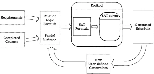
Partial Instance New User-defined ConstraintsFigure 1-1: Data flow in course scheduling system
Figure 1-1 gives an overview of our system's functionality. The targeted user of the system is a student looking to generate a schedule for future semesters. This user supplies a set of courses he has completed and selects a set of requirements for the desired degree. The requirements may be supplied by the student himself or another person; the system has been packaged with requirements for several degree programs at the Massachusetts Institute of Technology. The requirements are used to generate a relational formula, while the set of completed courses is used to construct a partial
instance. A partial instance consists of mappings from relations to tuples that they
are known to contain, and aids in reducing the number of unknowns in the analysis.
'In this thesis, we use the definition of relational logic as presented in [2]-that is, first-order logic with the extension of transitive closure.
Kodkod N /SAT solver SAT Formula Completed Courses EZZ~
Lz~
GeneratedScheduleNext, the system executes a solver, Kodkod [10], to find a solution to the for-mula. A solution is an assignment of relations to values allowed by their bounds that conforms to the original partial instance, and for which the formula evaluates to true. Kodkod converts the formula into SAT and executes a general-purpose SAT solver, such as ZChaff [7]. The solution returned by the SAT solver is translated back into a schedule and presented to the user. Through the interactive interface of our system, the user can proceed to add additional constraints to optimize the generated solution according to personal preferences; these constraints are conjoined to the original relational formula, and a new solution is generated.
Our strategy formalizes course scheduling as a satisfiability problem. Indeed, much research has been done to model planning as a satisfiability problem [5], and to automatically construct propositional SAT formulas from planning problems [3, 1]. Our approach differs in that the translation is done to relational logic, and the ability of Kodkod to accept partial instances is used whenever possible to reduce the number of variables in the generated formulas.2
1.2.1
Setting up the Problem
In this section, we will give an example of the system in action. To begin, the user selects a degree program whose requirements will be loaded into the system. The requirements are represented in an XML format (see Appendix A). Suppose the user has chosen the requirements for the Electrical Engineering and Computer Science
(EECS) Bachelor of Science program at the Massachusetts Institute of Technology.
These requirements encapsulate information about:
* Required core classes and electives for the degree. For instance, they specify that the EECS core classes 6.001, 6.002, 6.003, and 6.004, must be taken, and that at
2
The amount of time needed to find a solution to a SAT formula is strongly affected by the number of Boolean variables and propositional clauses in the formula. When translating relational logic into
SAT, a relation is decomposed into multiple Boolean variables. For instance, a binary relation from
a domain of m atoms to a range of n atoms is represented by a matrix of mxn variables; a variable xi evaluates to true if the ith atom in the domain and jth atom in the range are related. When Kodkod is supplied with a partial instance, it replaces such variables with constant Boolean values. If this were not possible, Kodkod would have to not only include extraneous variables but also add propositional clauses to constrain the variables' values.
least two of the three computer science "header" classes (introductory subjects for the three concentrations: Artificial Intelligence, Systems, and Theoretical Computer Science) must be completed.
9 Prerequisite relationships between individual classes. For example, the
prereq-uisites for 6.004 (computer architecture) are 6.001 (computer programs) and
6.002 (circuits). Certain courses' prerequisite requirements may be satisfied in
more than one way. For instance, 6.002's prerequisites are one of 18.03/18.06 (differential equations/linear algebra) and one of 8.02/8.022 (variations of elec-tricity and magnetism offerings).
In addition to course requirements, the user gives the system a set of completed courses. These courses can be used to satisfy prerequisite or degree requirements. Completed courses may be entered manually or imported from an HTML grade report file produced by the MIT Student Information System (http://student.mit.edu).
1.2.2
Converting to Relational Logic
To represent the course scheduling problem, we define a set of relations and constrain the values that can be bounded to each relation with partial instances and formulas. The details of this data model are explained in Chapter 2. Here, we will instead present a simple example that involves the following relations in the model:
" Semester: unary relation containing the set of semesters.
* Course: unary relation containing the set of all possible courses.
" sCourses: binary relation whose domain is Semester and range is Course.
sCourses contains a tuple (s, c) if c is scheduled for the semester s.
As an example, consider the requirement that the core courses 6.001, 6.002, 6.003, and 6.004 must be taken. To express this requirement, we write the following rela-tional formula (expressed in Alloy syntax [4]):
(6.001 + 6.002 + 6.003 + 6.004) in Semester.sCourses
The plus sign (+) and dot (.) between relations (i.e. not including a dot within a course number) denote union and join operations, respectively, while the keyword
in denotes subset of. Note that singleton unary relations must be created for each of
6.001, 6.002, etc. in order to be able to reference individual courses in a formula.
For each relation that is created, Kodkod requires that we specify an upper bound and optionally a lower bound of tuples. The upper bound of a relation consists of all tuples that may appear in the relation; the lower bound consists of all tuples that must appear in the relation. A partial solution can thus be set with the lower bound; knowl-edge that a course c must be scheduled in semester s can be handled by including the tuple (s, c) in the lower bound of sCourses. All courses that have already been com-pleted are mapped in this manner to a special semester called PastSemesters-this is done to distinguish courses that the user has already taken from courses generated
by the system and is helpful because we do not check if prerequisite relationships are
satisfied for the former (the user might have obtained special permission from the department).
Also note that lower bounds are used to completely define some relations; this happens when the lower and upper bounds are identical. Completely defining a relation eliminates the need for the external solver to determine its value from the formulas. For instance, Semester and Course, as well as the singleton course relations mentioned earlier, are set in this manner.
Prerequisites
To handle prerequisite relations, we define additional binary relations to map courses to their prerequisites. We then set the lower and upper bounds of these relations with the prerequisite information defined in the input. For example, we must bound the
appropriate relations with the information that 6.001 and 6.002 are prerequisites for 6.004.
Once the appropriate relations are pre-set with prerequisite relationships, the system can include a single formula to require that for any course appearing in Semester. sCourses, the course's prerequisites must be scheduled for a semester be-fore the one for which the course has been scheduled.
requirements for some courses can be satisfied in multiple ways. The details of how this is treated are discussed in Chapter 2.
1.2.3
Solving with Kodkod
Once the scheduling system has created a relational formula and bounds information, it executes Kodkod to generate a solution to the formula. If no solution is found, the user is alerted that there is no way to complete the degree (because the requirements are inconsistent, or because there are not enough semesters left to complete the de-gree, etc.). Otherwise, the solution is mapped back to the original planning problem; that is, we extract information from the values of the relations. The most important relation, as one might guess, is sCourses, which enumerates the generated schedule. In Chapter 2, we will illustrate how our data model allows further interesting informa-tion to be extracted; for instance, if a particular requirement, such as the computer science header requirement mentioned earlier, can be satisfied by two of three possible courses, it is possible to easily determine which two courses were actually chosen to satisfy this requirement without having to examine the entire generated schedule.
1.2.4
Viewing Solution and Adding Constraints
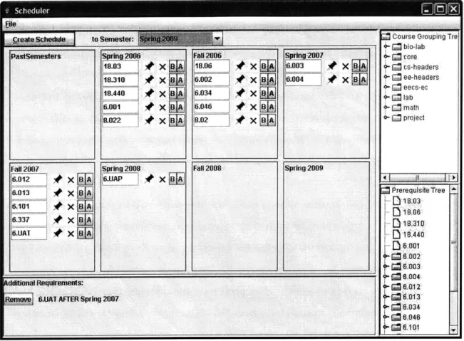
Figure 1-2 is a screenshot of the user interface for presenting a generated schedule. Courses are grouped by the semester to which they are assigned (for instance, 18.06 and 6.002 have been scheduled for Fall 2006), and the various buttons allow the user to add additional constraints to adjust the solution according to their personal preferences.
The user can, for example, require a certain course to be omitted from the schedule or to be scheduled only before/after a certain time. In the figure, such a requirement appears at the bottom panel; any new solution that is generated will include the course 6.UAT in a semester after Spring 2007. Detailed instructions for these and other features are given in the User Manual (Appendix C).
Figure 1-2: Example of generated solution, with an additional requirement
translated into relational logic and conjoined to the original formula created from course requirements. The solver is then re-run, and a new schedule is returned.
1.3
Contribution
This thesis presents a method for modeling planning problems as a relational for-mula with a partial instance. To our knowledge, although planning has often been modeled as satisfiability problems in other logics (e.g. propositional [5, 3, 1] and tem-poral [8]), the particular approach we use is uncommon. Using a relational model to represent our data allows our system to easily extract more useful information from the relational solution than just the generated schedule; for instance, the system can explain how particular requirements were satisfied in the generated schedule simply
by evaluating the appropriate relations. In addition to the representation benefits
of our approach, we show empirical results that, in the course scheduling domain, it is competitive with or exceeds the performance of general-purposes propositional solvers.
This method of translation is applicable not only to course scheduling but also for providing a platform to solve other planning problems with minor modification. Planning problems exist in domains such as manufacturing and transportation, and may appear in the form of order precedence and resource capacity constraints, for example.
This thesis also presents an expressive but simple syntax for formalizing course requirements. For this particular domain, general-purpose planning languages can be overwhelming and/or awkward to use for specifying input by a user not well-versed in discrete mathematics, so a domain-specific language is desirable.
Finally, this thesis embodies a fully functional system for creating course schedules that will hopefully be of use to students at the Massachusetts Institute of Technology
Chapter 2
Data Model and Representation
In this chapter, we discuss our relational logic representation of course scheduling. We begin with an overview of the model and subsequently detail the translation mechanism for different types of requirements.
To illustrate our data model, we will provide examples from the Department of Electrical Engineering and Computer Science at the Massachusetts Institute of Technology. Most MIT courses are numbered in the format X. Y where X is the department number (e.g. '6' for EECS) and Y is the subject number.
2.1
Relational Model
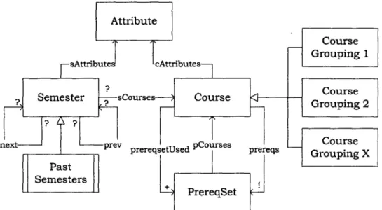
Figure 2-1 depicts the relations used in our representation. The boxes represent unary relations (i.e. sets) while the labeled arrows represent binary relations between sets. The open-ended arrows represent a subset relationship. Finally, the multiplicity markers ?, !, and + denote zero or one, exactly one, and at least one, respectively.
The following is a hierarchical description of the relations.
" Attribute-an attribute, such as Spring or Even (year, e.g. 2006), that can
be assigned to a particular Course or Semester.
" PrereqSet-a set of courses, such as {6.001,6.002}, that together can ful-fill the prerequisite requirements of a particular course. Note that PrereqSet
Attribute
sAttributes TcAttributes
Semester sCourses--- Course
next- prev prereqsetUsed PCOurses
prereqs Past Semesters - PrereqSet Course Grouping 1 Course Grouping 2 Course GroupingXj
Figure 2-1: Object model
- pCourses maps a PrereqSet to the courses it a prerequisite set P that represents the courses mapped by the pCourses tuples (P, 6.001) and
contains. For instance,
6.001 and 6.002 will be
((P,6.002).
" Course-represents a single course, such as 6.002.
- cAttributes maps a course to its attributes, with tuples such as (6.033, Spring), which indicates that 6.033 is only offered in spring semesters.
- prereqs indicates which PrereqSet(s) may be used to satisfy a course's prerequisite requirements. Courses that do not have prerequisites are mapped to the empty set {}.
- prereqsetUsed represents the one prerequisite set that is used to satisfy a course's requirements in the generated schedule; this is useful in the event that a course is mapped to multiple possible PrereqSets by prereqs.
- Course Groupings are subsets of Course that are created during
transla-tion for writing more expressive constraints. A course grouping may or may not be a singleton set. See Section 2.2 for details.
* Semester-denotes a single semester. PastSemesters is a singleton subset of Semesters and is used to represent the amalgam of all semesters in the past.
- prev and next denote the ordering of elements of Semester. For instance, prev might have the tuple (Fa112006, Spring2006), and next would then
contain the tuple (Spring2006,Fa112006).
- sCourses maps a semester to the set of Courses scheduled for it.
2.1.1
Discussion
Attributes
Attributes were designed as a simple way of indicating that not all courses are offered every semester. If a course has a specific attribute, such as Spring, then our con-straints will require that it be scheduled only to a semester that also possesses this attribute (see Section 2.2.2). This mechanism is also used to handle the common case of a course that is offered every other year, and can also be used for one-time course offerings (by defining a unique attribute).
Course Groupings
A course grouping is a unary relation that represents some arbitrary set of courses. It
is created during translation into relational logic to allow formulas to directly reference this arbitrary set. When the user defines a course grouping, he must also provide a set of requirements to constrain the values that the set can take. For example, consider the requirement that at least two of the three MIT computer science "headers" (6.033, 6.034, 6.046) must be taken. The user can define a course grouping named "cs-headers" and include the requirement that two of three courses must be in the course grouping, and the system will appropriately generate a relational formula from the requirement to constrain the relation cs-headers. The purpose of creating such a grouping is so that the user can easily refer to the set of selected computer science headers when writing other requirements.
For instance, suppose in addition to the header requirement above, the student is required to take two elective courses. The elective courses may be chosen from the headers and a selection of intermediate and advanced courses, but the same course may not be used to fulfill both the header and elective requirements. Thus, it is useful to be able to write a constraint that can refer to the two course groupings that satisfy
each of these requirements and require that they do not intersect.
Single-course course groupings are a special case. These are simply course
group-ings that are created to represent not an arbitrary set of courses, but instead ex-actly one course. For instance, consider the constraint that the set of scheduled courses must contain 6.001. When our system translates this into relational logic, it becomes 6.001 in Semester. sCourses. This requires a singleton unary relation named 6.001 that contains only the course 6.001. Thus, for every course, we create such "single-course" relations.
Prerequisite Sets
The notion of prerequisite sets was introduced to allow for courses whose prerequisite requirements can be satisfied in multiple ways. Usually, the department denotes this as a conjunction of disjunctions; for instance, in MIT's Electrical Engineering and Computer Science curriculum, the circuits course 6.002's prerequisites are one of
18.03/18.06 (differential equations/linear algebra) and one of 8.02/8.022 (variations of
electricity and magnetism offerings). In contrast, our representation is a disjunction of conjunctions. The same requirement can be rewritten as one requiring that any one of the four sets {18.03,8.02}, {18.03,8.022}, {18.06,8.02}, and {18.06,8.022} must be taken. As we will see in section 2.2.3, this representation allows for a simple way of expressing prerequisite constraints in relational logic.
2.2
Requirement Translation
In this section, we will describe the details of translating user-specified scheduling constraints into the above representation.
Translation has the following steps:
1. Allocate course grouping relations depending on the requirements.
2. Create bounds (including partial instances, if applicable) for all relations.
2.2.1
Using Partial Instance Functionality
Kodkod, the relational logic constraint solver used in our system, supports the notion of a partial instance. For each relation, we must specify an upper bound and optionally a lower bound of tuples. The upper bound of a relation consists of all tuples that may appear in the relation; the lower bound set consists of all tuples that must appear in the relation. A partial instance can thus be set with a non-empty lower bound.
Furthermore, we can completely define the value of a relation by setting identical lower and upper bounds. Doing so eliminates the need for the external solver to determine the relation's value from the formulas.
The following relations are completely defined prior to solving:
" The "Types": Attribute, Course, PrereqSet, Semester. " PastSemesters.
" Single-course course groupings.
" prereqs, pCourses. * next, prev.
" cAttributes, sAttributes.
If the user has entered a set of courses that he has taken in the past or wants to
fix parts of his future schedule (e.g. to require a specific course to be scheduled for a certain time), we specify these constraints by setting a non-empty lower bound for sCourses.
2.2.2
Global Constraints
Matching Attributes
As mentioned in Section 2.1.1, we constrain the the model so that a course is only ever assigned to a semester that has the course's attributes. The formula is as follows:
pred attributesMatchO {
all s : Semester - PastSemesters I
s.sCourses.cAttributes in s.sAttributes }
Preventing Schedule Overlap
The relation sCourses needs to be constrained so that a course is not assigned to multiple semesters. This can be done as follows:
pred noOverlap() {
all si : Semester I all s2 : (Semester - si) I
no (sl.sCourses & s2.sCourses)
}
No semester skipping
Finally, the system should not generate a schedule that contains "skipped" semesters, i.e. an empty semester before a non-empty one, unless that semester is the special PastSemesters, whose courses are user-specified. The constraint can be written as
follows:
pred noSemesterSkipping() {
all si : (Semester - PastSemesters) I all s2 : (si.^prev - PastSemesters) I
some sl.sCourses => some s2.sCourses
}
where ^ denotes the transitive closure operation.
2.2.3
Prerequisite Translation
The first step of prerequisite translation is completely defining the values of the rela-tions prereqs and pCourses, to represent the user-provided prerequisite relarela-tionships between courses. This, as mentioned previously, is done by setting identical lower and upper bounds for these relations.
Next, we need to bound the prereqsetUsed relation. Its upper bound is the same as that of prereqs. In addition to that, we add a logical formula to constrain that preresetUsed is a function with domain Semester. sCourses and range PrereqSet. Thus, for any scheduled course, prereqsetUsed will "choose" one of its valid prereq-uisite sets.
The next step is to generate the logical formulas to constrain sCourses so that for every scheduled course, the courses in its chosen prerequisite set, as specified in prereqsetUsed, are scheduled to be taken in a previous semester. This can be expressed in relational logic as follows:
pred prereqConstraint() {
prereqsetUsed.pCourses in ~sCourses. prev.sCourses }
where ~ denotes the transpose operation.
2.2.4
Degree and Additional Constraint Translation
As discussed in Appendix A, our system will translate, in addition to prerequisites, degree requirements and also additional constraints not specific to the degree program (such as user preferences).
Degree requirements are specified as a set of conjoined requirements that constrain the special course grouping corresponding to the expression Semester. sCourses, as well as requirements to constrain any other course groupings that are defined and referenced. Additional requirements are a conjoined set of standalone requirements.
Modularity of Translation
A major benefit of course groupings (discussed in Section 2.1.1) is that they allow for
the modular translation of requirements. Although the requirements that constrain a course grouping C1 may reference another course grouping C2, the translation of these requirements do not depend on the requirements that constrain C2; when we reference the relation corresponding to C2, we can assume that this relation will be properly constrained when C2's requirements are translated. Thus, we can group translation of requirements by the course groupings they constrain. Standalone requirements can be translated independently.
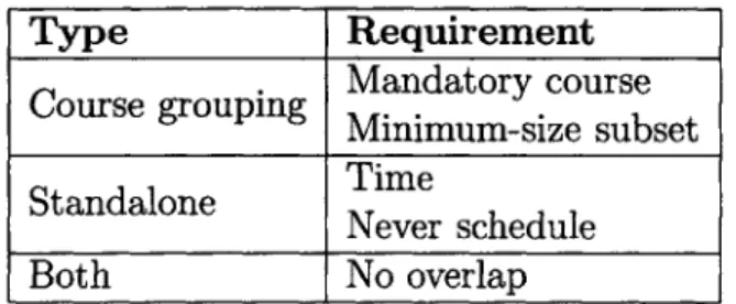
Type Requirement Mandatory course Minimum-size subset Standalone Time Never schedule Both No overlap
Table 2.1: Supported requirements.
Translation by Requirement Type
Table 2.1 summarizes the set of requirements we support. Certain requirements must occur in the context of a course grouping definition, while others must be standalone. When a requirement is part of a course grouping's definition, we call that grouping the requirement's subject.
Mandatory course requirement
A mandatory course requirement indicates that a desired set of course groupings must
appear in the subject; this can be written as a simple subset formula.
Input: Course groupings c1, c2, ... ,c must appear in subject S.
Formula: cl+c2+. .. +cn in S
Table 2.2: Mandatory course requirement translation
Minimum-size subset requirement
A minimum-size subset requirement indicates that at least some number (k) of a
selection of course groupings must appear in the subject. There are a number of ways to translate this. Assuming the set of allowed course groupings is of size n, one approach is to enumerate all
(n)
subsets of size k, write a subset formula for each of them, and take the logical disjunction.As we will discuss in Section 4.1, this approach is inefficient for values of n and k sometimes encountered in practice (e.g. n = 80, k = 2). However, assuming that all n
Input: At least k of the n course groupings ci, c2, ... , c must appear in subject S.
Formula: (K1 in S) II (K2 in S) II ... II (Kx in S), where each Ki is a unique union of k members of the set of course grouping choices, and
Table 2.3: Minimum-size subset requirement translation (general case)
can instead use a substantially more efficient translation with an existential formula. Note that whereas the number of clauses in the general translation above is linear in
(, in the translation below it is linear in
Q),
which in practice is much smaller. Input: At least k of the n course groupings ci, c2, .. , cn must appear in subjectS.
Formula: some v1,v2,. ..,vk: (c1+c2+.. .+cn) I (vl+v2+.. .+vk) in
S && (no Il) && (no 12) &&... .&& (no Ix), where each Ij is a unique pairwise intersection of the quantified variables vi (e.g.
(vl&v2), (v2&vk)), and x= ().
Table 2.4: Minimum-size subset requirement translation (all single-course case)
No overlap requirement
A no-overlap requirement simply states that none of the course groupings it specifies
can have overlapping values; that is, the same course must not appear multiple times. If the requirement is part of a grouping's definition, that grouping will be included in the constraint. The translation is a conjunction of empty pairwise intersection constraints.
Input: The course groupings c1, c2, ... , cn, and the subject S, if applicable, must not have overlapping values.
Formula: (no P1) && (no P2) && ... && (no Px), where each P is a unique
pairwise intersection (e.g. (cl&c2), (cl&cn)), and x = ().
Time requirement
A time requirement indicates that a course must be scheduled before, at, or after a
specified semester. A before/after requirement is written as a formula in relational logic. Note that unlike the requirements described earlier, the input to a time re-quirement is a course, not a course grouping.
Input: The course c must be scheduled to be taken before semester S. Formula: c in S. ^prev.sCourses
Table 2.6: Time requirement (before) requirement translation
Input: The course c must be scheduled to be taken after semester S. Formula: c in S. next.sCourses
Table 2.7: Time requirement (after) requirement translation
Notice that this translation requires that c be scheduled (as opposed to only requiring that the timing constraints be satisfied when the course is in fact scheduled). This is consistent with our definition of the requirement as described in Appendix A. While it is possible to also translate the requirement that a course be taken exactly at a particular time into a relational formula, we instead take advantage of the partial instance functionality of Kodkod and do something simpler-include the (semester,
course) tuple in lower bound of the relation sCourses.
Never schedule requirement
We can require that a course not be scheduled to any semester with a simple formula. Again note that the input to this requirement is a course, not a course grouping.
Input: The course c must not be scheduled to be taken in any semester. Formula: not (c in Semester.sCourses)
Chapter 3
System Architecture
3.1
Overview
Our scheduler system was written in approximately 6500 lines of Java 1.5 code. It uses the relational constraint solver Kodkod, which is also Java-based, and various external Java libraries for HTML parsing and graphical user interface layout.
There are two versions of the system: a web service and a standalone applica-tion; the web service performs the resource-intensive processing on a server. In both versions, the user interacts with the system through a common Swing graphical user interface. In the case of the web service, the interface is part of a Java applet within a web page.
3.2
Key Data Abstractions
We now describe the key data types in the system. Note that many of these types can be serialized into XML. This simplifies remote execution as most code from the standalone version can be reused, and the only things that need to be added are wrappers that serialize, transfer, and deserialize XML (see Section 3.4).
3.2.1
Semester, Course, Attribute
These basic data types are implemented as Java classes and are instantiated to repre-sent atoms in our system's relational data model (described in Section 2.1). The data model defined a fourth basic type-PrereqSet. In the implementation, we simply represent a PrereqSet atom as a parameterized Java Set of Course objects.
3.2.2
Schedule
This is a simple hashtable data structure that stores the set of courses allocated to each semester and an ordering over the set of semesters. The class is used to represent both an initial schedule of completed courses provided by the user and a final schedule generated by the system.
3.2.3
CourseGrouping
This class represents the concept of a course grouping in our relational model, as defined in 2.1.1. Each instance of CourseGrouping corresponds to one arbitrary set in the data model, and contains its name and the set of Requirements that define
(constrain) the course grouping.
3.2.4
Requirement
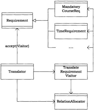
Requirement is an interface that must be implemented by all requirement types, whether it be standalone or part of a course grouping definition. The interface con-tains a single method, accept O, for accepting visitors, as is common when using the common Visitor design pattern. Each instance of Requirement should represent a concrete constraint specified by the user. For instance, the requirement that a course
6.001 must be taken is represented as an instance of the class MandatoryCourseReq,
which implements Requirement.
Different types of requirements should be implemented as distinct subtypes of Requirement. For instance, each requirement type listed in the translation rules in
Section 2.2.4 is implemented as a separate class in our system. This allows for a modular requirement translation mechanism, as described in Section 3.3.
3.2.5
DegreeProgram
A DegreeProgram is an abstraction for the requirements needed to complete a
de-gree and contains a set of CourseGrouping objects (each of which contains a set of Requirements). DegreeProgram must include a special CourseGrouping instance that corresponds to the set of all scheduled courses (the expression Semester .sCourses in our relational model).
3.2.6
PrereqMap
This map-like data structure stores the prerequisite sets for each course. Prerequisite sets may be added to a course and retrieved for one in constant expected time.
3.2.7
Problem, Solution
A Problem object packages all the requirements (regarding the degree program,
pre-requisite relationships, and any additional standalone constraints) that will be passed to the backend. Thus, an XML serialization of this type is self-sufficient for archiving a query.
Solution is an interface for representing a solution generated by the system and contains methods for accessing the generated schedule and extracting values of indi-vidual course groupings and information from other relations (e.g. prereqsetUsed-see Section 2.1.).
3.3
Translation Architecture
Translation involves two steps: the allocation of relations and the translation of re-quirements into the relational model. The output at the end of the translation process
is a relational formula object created using Kodkod's API, as well as upper and lower bound information for the relations that are referenced in the
Mandatory
L
CourseReq Requirement <-TimeRequirement accept(Visitor) Translate Translator Requirement Visitor ) RelationAllocatorFigure 3-1: Requirement translation dependency diagram.
Figure 3-1 shows a dependency diagram of the classes that perform the trans-lation. The Translator class is the central controller for translation and invokes the RelationAllocator to allocate relation objects for use in the relational for-mula. After allocation, the Translator creates upper and possibly lower bounds for each relation, in the manner described in Section 2.2.1. Finally, it invokes the class TranslateRequirementVisitor to translate each requirement that is encountered, either in a standalone context or in the definition of a CourseGrouping; the formula translations of the requirements are conjoined to the global constraints (described in Section 2.2.2) and returned as a single formula. Note that TranslateRequirementVisitor depends on RelationAllocator, for retrieving references to the allocated relation ob-jects (corresponding to a particular course grouping, for instance).
TranslateRequirementVisitor implements the RequirementVisitor interface, which contains overloaded visit () methods to accept each subtype of Requirement as an argument and return a value, in this case a relational formula object representing
the visited requirement.
For instance, the aforementioned MandatoryCourseReq requiring 6.001 to be taken would be handled by a method with signature visit (MandatoryCourseReq), which would examine the requirement object, and return the appropriate subset formula.
To support a new requirement type, a developer would simply need to augment RequirementVisitor and TranslateRequirementVisitor to contain a visit 0 method for the new type. The rest of the translation system can remain unchanged.
3.4
Remote Execution Architecture
The web service version of our system delegates the resource-intensive processing to a remote server; specifically, the translation of a Problem into relational logic and the execution of Kodkod run remotely. We use Java servlets, hosted on the Apache Tomcat web server, to support remote execution in our system. A Java servlet is a class on the server that can listen to an HTTP connection and process GET/POST requests. The advantage of Java servlets is that they are in pure Java-servlets can easily be integrated with other parts of the system and invoke the same code as a local Java application. This allows the standalone and web service versions of our system to share not only essentially all front-end (user interface) code, but also much of the translation and solving back-end.
Kodkod
Formula, Instance Bounds
Problem-- Translator
-Solution-Figure 3-2: Local execution architecture.
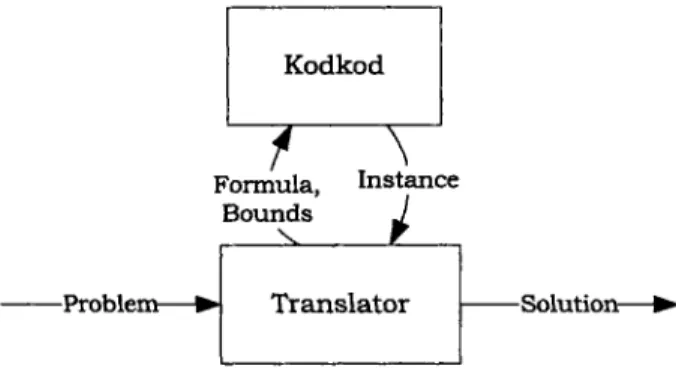
To see the differences between the two versions of the system, first consider the architecture for the standalone version (Figure 3-2). A Problem object is passed to
the Translator class, which invokes Kodkod and converts the returned instance (that is, a satisfying model of tuple assignments to relations) into a Solution.
Remote Server Formula, Translator Bounds Kodkod I Problem Solver Instance I Serviet HTTP Post Instance (Problem XML) JavnalMap
Prbeka Problem -Problem HTTP Instance Seoltoe outo--Problem Writer (XML) Message (Java Map)-1 Solton -Solution
Factory
Figure 3-3: Remote execution architecture.
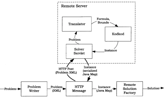
The analogous architecture for the web service is shown in Figure 3-3. The Problem object is first converted into XML, and then passed to a HTTP request sender called HTTPMessage. An HTTP/POST request is sent to the server and han-dled by the SolverServiet class, which invokes the Translator and Kodkod in the same manner as before. The instance returned by Kodkod is converted into a String-based Java Map (that maps from relation names to its tuples) and sent back as an HTTP response. RemoteSolutionFactory is run locally on this response and wraps it in the Solution interface.
3.4.1
Alternative Design
It would have arguably been more uniform to develop an XML serialization for the Solution interface and, for the HTTP response, simply construct an instance of Solution remotely and return its XML serialization. The primary disadvantage of
this approach is that the efficiency of a data structure like Java's Map or Kodkod's Instance, which are suitable for handling many retrieval requests, is lost. On the other hand, having XML functionality for Solution would have the advantage of enabling the user to record the system's output, but this loss is not very significant because we already support XML serialization of the generated Schedule, which is the most important part of a Solution.
Chapter 4
Evaluation
4.1
Performance
As our system is meant for practical usage by students, it is imperative that it shows reasonable performance, both in its speed and in the quality of results it returns.
We performed empirical tests with two example degree programs, one for the Bachelor of Science (SB) degree in Electrical Engineering and Computer Science from MIT, and the other for the Master of Engineering (MEng) degree in the same de-partment. Despite its name, the latter is actually a combination degree that includes the former's coursework as a subset, but additionally contains substantially more complicated logic for requiring electives from varying concentrations. With the opti-mizations described in this section (some of which actually sacrifice running time for more desirable output), the system finds a schedule for the SB program in 4.9 seconds and for the MEng program in 8.6 seconds on a 2.8GHz Intel Pentium 4 machine with 1GB of RAM.1 Our system can be expected to run in similar times for most other degree programs.
'All reported computation times in this chapter were run with a scope of 8 semesters and no
completed courses on Sun's Java 1.5 JDK for Windows XP. Interestingly, running with a set of
completed courses does not seem to affect the speed by a noticeable amount.
The JVM was run with a maximum heap size of 128MB. The standalone version of the application was used, but the remote execution overhead for the web version is usually no more than a second.
4.1.1
Minimum-size Subset Requirements
A big hurdle that we faced was the poor performance of the original minimum-size
subset requirement translation, and various alternatives were considered. As discussed in Section 2.2.4, the general case translation for this type of requirement creates a clause for each of the
(n)
subsets of size k from the n choices. This requirement type is often used to express the notion of "elective courses" in a degree (i.e. courses that are optional individually but of which at least a fixed number must be taken). A typical elective constraint may have n and k of 80 and 2, respectively, and generating(0)
= 3160 clauses in the formula and translating them into SAT takes a prohibitiveamount of time (> 60 seconds for the MEng degree program; the exact range depends on what other optimizations are used in combination.). The translation also requires more memory than usual; both the Java heap and stack sizes needed to be increased to handle the deeply nested conjunction.
As we described previously, if all the choices allowed by the requirement were single-course course groupings, we could use a far more efficient translation involving existential quantifiers. The efficiency of this approach relies on the fact that ex-istentially quantified formulas can be "skolemized" [2]. Normally, when a relational formula is translated into propositional logic for use in a SAT solver, quantified formu-las are "grounded out," which is a method used in bounded first order logic analysis to convert a quantified formula into a conjunction (for a universal quantification) or disjunction (for an existential quantification) of propositional clauses. For instance, consider the existential quantified formula some x: X I P x). Assuming X has an upper bound consisting of the atoms xo and x1, then the quantified formula can be grounded out into P(x) II P(x).
Skolemization involves recognizing that we can express the same requirement by explicitly defining a singleton unary relation x' to be a subset of X and including the single propositional clause P(x'). If the model finder (solver) can find a model (solution) that satisfies this formula, then the value of x' must be an element of X that satisfies P, and proves the existential formula. If the solver cannot find any
satisfying solution, then it proves the existential formula to be false for the given bounds of X. One can see that the skolemization is constant in n (the size of X) and far more efficient than grounding out, which is linear in n.
Assuming the "solution pruning" method for minimality (described in the next section) is used, changing from the general translation to the existential translation for the single-course case reduces the running time of our system for the SB program from
7.0 seconds to the 4.9 seconds stated above, and the MEng program from essentially
unsolvable to the 8.6 seconds from above.
However, note that if an existential quantified formula appears in the context of a negated formula, then it can no longer be skolemized and instead must be grounded out. Local minimality constraints, described in Section 4.1.2, do in fact negate a requirement's translation, so the effect of grounding out is an issue there. We will see that the aforementioned "solution pruning" method attempts to resolve some of these issues.
Finally, instead of existential formulas, if our solver supported primitive handling of set cardinality expressions, then minimum-size subset requirements would be trivial to translate, and should scale just as well as the skolemized existential formulas, without the danger of needing to be grounded out.
4.1.2
Minimality
The issue of minimality proved to be one of the most challenging parts of our sys-tem's development. Since we model course scheduling as a satisfiability problem, our system may return a solution that, while satisfying the course requirements, is less desirable than other possible solutions. A common, and the most serious, such type of undesirable solution is one that contains too many courses. In fact, if we do not ex-plicitly try to restrict the size of the generated schedule in our relational formula, our system will almost always return a schedule that has more courses than is practical (e.g. for instance, more than ten per semester).
There are at least four ways in which we could control this problem:
car-dinalities, we could set a hard limit on the size of the set of courses that are scheduled.
2. Without built-in cardinality expressions, we could try to emulate their support with relations (see description below).
3. We could add an optimality constraint to the relational formula so that any
generated instance must satisfy the constraint.
4. We could prune an oversized solution to get rid of extraneous courses.
Using Set Cardinality
When we encountered this problem, the first option was out of the question because Kodkod did not yet have support for cardinality expressions. A prototype of the sec-ond option was attempted, but, not surprisingly, it proved to be impractical (running for minutes without halting). We created a unary relation of positive integers and a ternary relation of type Semester->Course->Integer to index each course scheduled for a semester. We also created a binary inc relation between integers to represent their natural ordering. The idea is that we can determine the number of courses assigned to each semester by seeing how "far" its indexing goes. Even if we cap the maximum possible index to a small number like ten, with more than 250 courses and a typical number of 6 semesters, the relation size blows up, and quantified formulas to constrain the indexing relation in useful ways become a bottleneck to translate into SAT. Moreover, even simple expressions containing that relation would be more time consuming to translate than most other expressions.
There is another problem with both of the set cardinality approaches. When given a cap on the number of courses that can be scheduled, it is probable that the system would return solutions that have exactly or close to the maximum size. Thus, depending on what we specify the maximum to be, the solution would still potentially have a significant number of extraneous courses, or worse yet, if we set the maximum to be too small, the system would not be able to find a solution.
An alternative would be to begin with a low maximum value, run the solver, and if a solution could be found, increment the maximum, rerun the solver, and repeat
until one was returned (or use some other searching mechanism, e.g. binary search, to find the correct maximum instead of fixed incrementation). This approach has two primary problems: first, the expected number of searches must be small (e.g. 3) to be comparable in speed to another approach we will describe below, and second, the method must be able to cope with the fact that the lack of a solution can indicate an overly low maximum or instead an overconstraint in other parts of the input (e.g. an unsatisfiable inconsistency in the requirements). The simplest way to handle the latter would be to have the system give up after a fixed number of retries, but that would be undesirable in speed and potentially in correctness.
Using Optimality Constraints
A well-written optimality constraint has the advantage of scheduling few or no
extra-neous courses. The approach we take is to require local minimality. The idea is to ensure that the generated solution cannot be reduced in size by removing any single course in it and still satisfy all the specified requirements. In relational logic, for each non-single-course course grouping G which must satisfy a predicate P(G) (from its definition), we conjoin the following formula to P(G):
all c: G I not P(G-c)
For the special course grouping corresponding to the entire set of scheduled courses, Semester. sCourses, we must do something slightly different because the minimality formula must be aware of the prerequisite constraints put on the schedule denoted by the sCourses relation. Assuming the user-defined requirements on Semester. sCourses
are translated into relational logic as the predicate P, we conjoin the following formula to P(Semester.sCourses):
all c: (Semester-PastSemesters).sCourses
I
not (P(Semester.sCourses-c) &&
((Semester-PastSemesters) .sCourses-c) .prereqsetUsed. pCourses
in (Semester.sCourses-c))
There are two caveats. First, a local minimality constraint of this type does not always generate minimally-sized schedules. For instance, consider a solution that
used a course X to satisfy a certain degree requirement, when Y could have been used instead. Suppose X had a prerequisite X', and Y had no prerequisites. Then, even though the generated solution was not minimal (X and X' could have been replaced by Y), it would still satisfy local minimality constraints in the above form because removing X would violate the mandatory course requirement, and removing X' would violate the prerequisite requirement of X.
Secondly, the modularity of course grouping translation (as discussed in Section 2.2.4) actually poses a problem in this approach because each course grouping's local minimality is considered independently. A course grouping generally represents a specific requirement in the degree program; often times, two requirements could be satisfied in a synergistic way, but considering the local minimality of the corresponding course groupings separately would not take this possible synergy into account. For instance, suppose there are two course groupings A and B, each of which could be satisfied in a number of ways, but one configuration allowed A's courses to be used as prerequisites for B's courses, thus eliminating the need to schedule extra courses to satisfy B's prerequisites. Our approach would not be aware of this and would only select courses to locally minimize the sizes of A and B.
In spite of these deficiencies, this approach is satisfactory in generating reasonably-sized schedules in practice. It does, however, increase processing time by a sig-nificant amount. The reason is that a university quantified formula for local min-imality may take a substantial amount of time to ground out. Consider the lo-cal minimality formula for Semester. sCourses presented above. The expression (Semester-PastSemesters) . sCourses has an upper bound that is the range of the relation sCourses (i.e. the set of all courses). For a typical analysis, there are over
250 courses, and grounding out becomes a significant bottleneck in our analysis. The
increase in processing time by adding the minimality constraints is particularly egre-gious when the existential translation for single-course minimum-size subset require-ments is used since, as suggested earlier, the existential formulas would no longer be skolemizable in the context of a negation and thus would take a lot of time to ground out. In fact, whereas running the system for the SB program with no
opti-mizations takes 3.7 seconds, with local optimality constraints, it takes 20.1 seconds; for the MEng case, where there are even more existential quantifiers, the running time increases from 5.4 seconds with no optimizations to over 70 seconds with the local minimality constraints added. It is interesting to note that, once grounded out, the resulting propositional formula takes a negligible amount of time to solve using a SAT solver. (This means that if we were able to use cardinality expressions to translate minimum-size subset requirements, then we would not expect to experience as significant of an increase in running time, as there would be less grounding out needed.)
Pruning an Existing Solution
The next method we propose extensively uses the partial instance functionality of Kodkod and improves in speed compared to the local minimality method above while retaining most of the latter's benefits. The idea is to first run the solver without minimality constraints to receive a bloated solution and then prune this solution.
Clearly, the pruning process must be fast. Pruning is done by executing the solver a second time, now with the local minimality constraints in place for non-single-course course groupings, as above. This may seem counterintuitive, as the whole point of pruning was to avoid the expensive quantification brought about by local minimality constraints. However, the reason we can now reduce the solving time is because the first solution will be used as a partial instance for the second run. Specifically, the tuples of relations corresponding to course groupings and of the binary relation sCourses will be used as the upper bounds of those relations in the second trial. In practice, this dramatically reduces the time needed for grounding out because the universe of quantification goes from over 250 courses to approximately 80 for the range of sCourses and single-digit sizes for course grouping relations (the latter of which may be the range of an existential quantifier for a minimum-size subset requirement). In fact, the reduction in solving time is so dramatic that with the combination of this pruning technique and the existential translation for minimum-size subset requirements, we achieve the user-friendly solving times noted at the