Decoding Team Performance in a Self-Organizing
Collaboration Network using Community
Structure
by
Israel Louis Donato Ridgley
B.S., Massachusetts Institute of Technology (2017)
Submitted to the Department of Electrical Engineering and Computer
Science
in partial fulfillment of the requirements for the degree of
Master of Engineering in Electrical Engineering and Computer Science
at the
MASSACHUSETTS INSTITUTE OF TECHNOLOGY
September 2018
c
Massachusetts Institute of Technology 2018. All rights reserved.
Author . . . .
Department of Electrical Engineering and Computer Science
August 21, 2018
Certified by . . . .
Patrick Jaillet
Associate Professor
Thesis Supervisor
Certified by . . . .
Troy Lau
PhD, Draper
Thesis Supervisor
Accepted by . . . .
Katrina LaCurtis
Chair, Master of Engineering Thesis Committee
Decoding Team Performance in a Self-Organizing
Collaboration Network using Community Structure
by
Israel Louis Donato Ridgley
Submitted to the Department of Electrical Engineering and Computer Science on August 21, 2018, in partial fulfillment of the
requirements for the degree of
Master of Engineering in Electrical Engineering and Computer Science
Abstract
When assembling a team, it is imperative to assess the ability of the team to perform the task in question and to compare the performance of potential teams. In this thesis, I investigate the predictive power of different community detection methods in determining team performance in the self-organizing Kaggle platform and find that my methodology can achieve an average accuracy of 57% when predicting the result of a competition while using no performance information to identify communities. First, I motivate our interest in team performance and why a network setting is use-ful, as well as present the Kaggle platform as a collaboration network of users on teams participating in competitions. Next, in order to identify communities, I ap-plied a selection of techniques to project the Kaggle network onto a team network and applied both spectral methods and DBSCAN to identify communities of teams while remaining ignorant of their performances. Finally, I generated cross-cluster perfor-mance distributions, evaluated the significance of communities found, and calculated a predictor statistic. Using holdout validation, I test and compare the merits of the different community detection methods and find that the Cosine Similarity in con-junction with spectral methods yields the best performance and provides an average accuracy of 57% when predicting the pairwise results of a competition.
Thesis Supervisor: Patrick Jaillet Title: Associate Professor
Thesis Supervisor: Troy Lau Title: PhD, Draper
Acknowledgments
I would like to thank my mother for her love and support throughout my life and my advisors Troy Lau and Patrick Jaillet for their invaluable guidance during the course of writing this Thesis.
This material is based upon work supported by the Air Force Research Laboratory (AFRL) and DARPA under United States Air Force contract number FA8750-17-C-0205.
Any opinions, findings and conclusions or recommendations expressed in this material are those of the author(s) and do not necessarily reflect the views of the United States Air Force or DARPA.
Contents
1 Introduction 13
1.1 Motivation . . . 13
1.2 Previous Work . . . 14
1.3 The Kaggle Platform . . . 15
1.4 Kaggle as a collaboration network . . . 15
2 Methods 21 2.1 Preprocessing . . . 23
2.1.1 General Preprocessing . . . 23
2.1.2 Version 1 and 2 Preprocessing . . . 24
2.2 Community Detection . . . 26
2.2.1 Projection Methods . . . 27
2.2.2 Clustering Algorithms . . . 29
2.3 Statistics and Analysis . . . 32
2.3.1 Cross-Cluster Statistics . . . 32
2.3.2 Clustering Significance Testing . . . 33
2.4 Holdout Prediction Testing . . . 34
2.4.1 Partial Holdout . . . 34
2.4.2 Whole Competition Holdout . . . 36
3 Results 37 3.1 Clustering Results . . . 37
3.1.2 Cluster Size Distribution . . . 39
3.1.3 Cluster Significance . . . 41
3.2 Holdout Testing . . . 41
3.2.1 Partial Holdout Testing . . . 41
3.2.2 Whole Competition Holdout . . . 45
List of Figures
1-1 Kaggle network example . . . 16
1-2 The ’Giant Component’ of the Kaggle Network . . . 18
1-3 A zoomed view of the lower right corner of the Kaggle Network . . . 19
2-1 Processing overview used to evaluate hypothesis. . . 21
2-2 Preprocessing Breakdown . . . 22
2-3 Community Detection Breakdown . . . 22
2-4 Statistics and Analysis Breakdown . . . 23
2-5 The ’Giant Component’ of the Kaggle Network using version 2 prepro-cessing . . . 25
2-6 Histogram of an example empirical cross-cluster score distribution. The x-axis is the score difference between a team in cluster A and a team in cluster B. . . 33
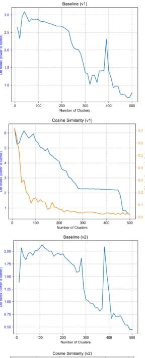
3-1 Results of clustering indices for version 1 and 2 preprocessing . . . 38
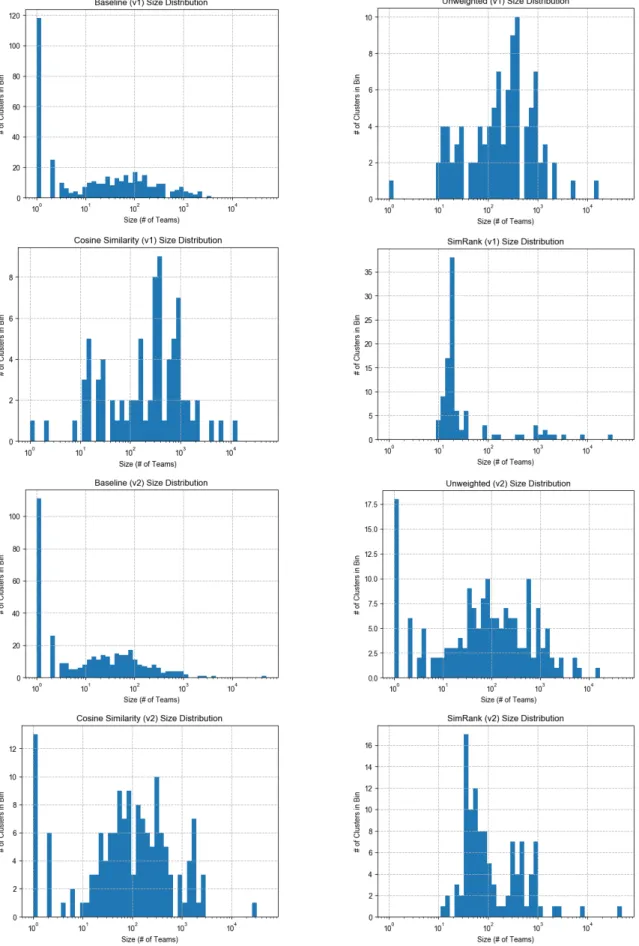
3-2 Size Distributions for version 1 and 2 preprocessing . . . 40
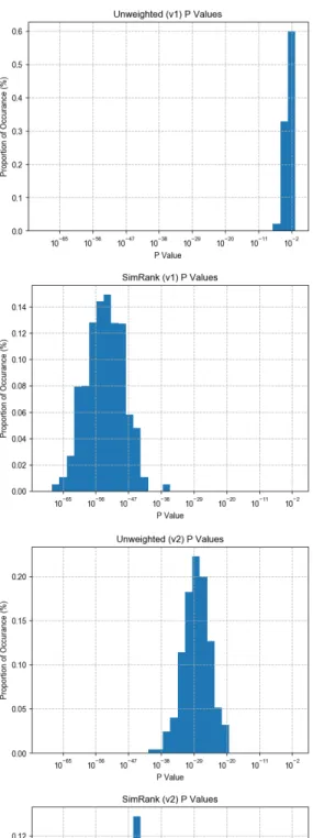
3-3 Results of partial holdout for version 1 and 2 preprocessing . . . 42
3-4 Results of partial holdout for version 1 and 2 preprocessing . . . 43
3-5 Results of partial holdout for version 1 and 2 preprocessing . . . 46
3-6 Results of complete holdout for version 1 and 2 preprocessing . . . . 48
3-7 Trend of complete holdout results with number of clusters for Cosine Similarity and SimRank . . . 49
List of Tables
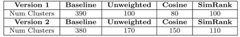
3.1 ’Optimal’ number of clusters for each method . . . 39 3.2 Details of partial holdout prediction testing for the version 1 projection
methods. All figures except for Accuracy are given as a percentage of N . 44 3.3 Details of partial holdout prediction testing for the version 2 projection
methods. All figures except for Accuracy are given as a percentage of N . 44 3.4 Details of complete holdout prediction testing for the version 1
projec-tion methods. All figures except for Accuracy are given as a percentage of N . . . 45 3.5 Details of complete holdout prediction testing for the version 2
projec-tion methods. All figures except for Accuracy are given as a percentage of N . . . 45
Chapter 1
Introduction
This Thesis represents work done over the better part of a year and explores the hy-pothesis that performance is encoded in the community structure of a self organizing network. The first chapter lays out the motivation and previous work done toward this hypothesis. This chapter also introduces the self-organizing network under study, the online data science platform Kaggle [12] as sourced through the Meta-Kaggle dataset [11], and discusses its merits, its formulation, and its caveats. The second chapter details the methodology used to transform and analyze this dataset, as well as the tests used to evaluate the hypothesis under consideration. The third chapter details the results from the methods section and the fourth chapter discusses these results, their implications to the hypothesis under consideration, and future work that would further illuminate the topic.
1.1
Motivation
Project managers, group leads, and coaches need to assemble the best team to accom-plish a task, be it producing high quality work, research, or winning a competition. The person forming the team may have a variety of options in deciding who to place on a team. It is therefore necessary to evaluate how different teams may perform relative to one another. If there is sufficient data available, say historic project teams and performance within an organization or recent world series teams and results,
then community detection may be a useful tool for finding sets of teams that perform reliably better or worse than one another.
My hypothesis assumes that structurally similar teams will perform similarly, and that by looking at the relative performance of teams similar to those in question, one can infer the relative performance of those that they care about. I experiment with different notions of structural similarity, the most successful of which is based off of the proportion of shared teammates. My assumption is supported by the success of my results but may require further work to verify unequivocally.
1.2
Previous Work
Collaboration networks are a form of complex networks [1, 2] that have been studied as a bipartite graph [20, 18] or a unipartite projection [1, 9] of a bipartite graph. Famous examples of collaboration networks include the Movie-Film network [1, 20] and the Scientific Author-Paper network [18]. Studies such as these that examine the abstract properties of collaboration networks are common; however, only a small minority of these studies consider the performance of entities embedded in these networks [9, 25]. Furthermore no studies found by this author form predictive models for performance based on network structure. My thesis is unique in that it is the first to use network structure in order to decode and predict the performance of teams within the network.
Another relevant field is the use of collaborative filtering in item recommendation systems [3, 23, 15]. Collaborative filtering uses a network of items and users which is very similar to the structure of a collaboration network. It also incorporates the notion of similarity in that similar users like similar products and that similar items are liked by similar users. In this way platforms and services can infer what item a user my like based on their and others previous interaction with items. Similarly this work hopes to infer how well a team will do based on the network of interactions on the Kaggle platform.
1.3
The Kaggle Platform
The Kaggle platform [12] hosts data science competitions created by both academia and industry, complete with the ability to form teams, a leaderboard to track progress, and, in many cases, a large cash prizepool. Kaggle is also home to a vibrant commu-nity of international data scientists that communicate and coordinate via the Kaggle forums, as well as share and analyze a diverse collection of datasets purely in the interest of discovery. Since the Kaggle platform is centered around data science, the Kaggle team generated a Meta-Kaggle dataset [11] containing a great deal of meta-data including which teams competed in which competitions, which users participated on which team, and the final leaderboard standings of each competition.
The Kaggle platform is an ideal place to test the hypothesis that network struc-ture encodes team performance since it has users who have substantial history on the platform, the freedom to form teams, an objective and numeric performance metric, and a variety of teams competing against each other in pursuit of a common objec-tive. Best of all, the Meta-Kaggle dataset is substantial – containing more than 300 competitions over the course of 6 years – and open to everyone.
1.4
Kaggle as a collaboration network
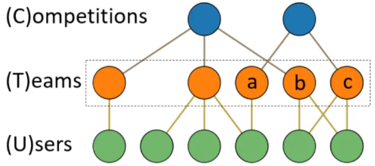
The Kaggle platform can be viewed as a collaboration network in which one set of nodes are users and the other set is teams. A link between a user and team represents participation of a user on a team. Competitions are included as a third node type in order to encapsulate another dimension to the collaboration network. There is a great variety of competitions on Kaggle, some of which require advanced skills such as Natural Language Processing or Video Processing. Given that competitions cover a variety of domains, it is reasonable to assume that teams and users who compete in many of the same competitions may have a similar skill set or proficiency.
Figure 1-1 shows a small scale example of the Kaggle network. Not shown are the links between users and competitions for legibility, however transitivity holds
Figure 1-1: Kaggle network example
and users are connected to the competitions that their teams compete in. Some idiosyncrasies of the data as presented by the Meta-Kaggle dataset are that teams, such as team ’a’ in Fig 1-1, can consist of a single user and that teams are unique to a competition, meaning that even though teams ’b’ and ’c’ share the same users they compete in different competitions and are thus unique. Due to this latter fact, every team in Meta-Kaggle has a unique score associated with it.
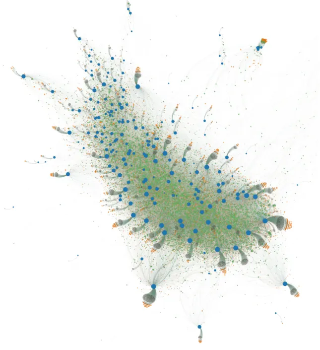
A large scale view of the Kaggle Network structure can be seen in Figure 1-2 where nodes are scaled by their degree, and competition, team, and user nodes are blue, orange, and green respectively. Note that this is not the entire network but only roughly 95% of it; the rest could not be displayed due to size constraints. Additionally I refer to the main mass of the network as the ’giant component’ even though some of the competitions cut off by the view presented are in fact connected to it.
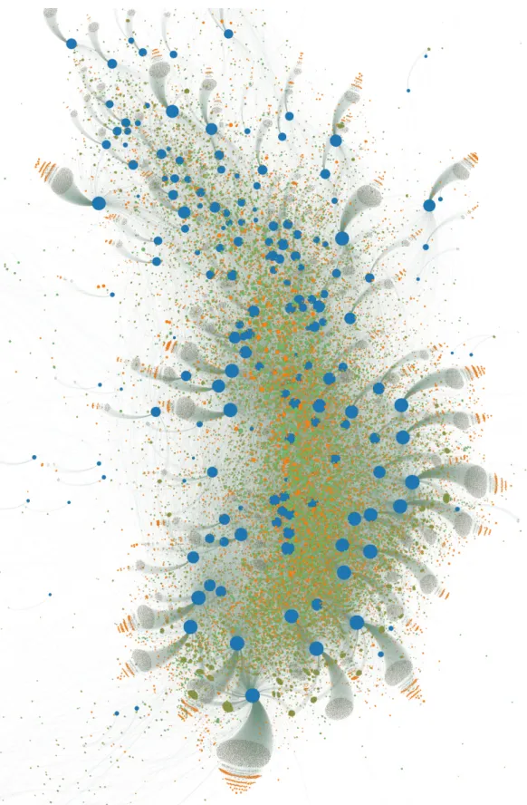
The Network consists of a core set of power users who compete in many compe-titions and are surrounded by the teams and compecompe-titions that they compete in. On the periphery of the giant component are competitions that have very little partici-pation by the power users. One can see this in more detail in Figure 1-3 where one can see that the competitions on the periphery have an ever larger set of users that are exclusive to them. The dark clouds attached to competitions are users with low degree, i.e. users who compete in the competition they appear next to and few if any other competitions as well as teams that consist only of them. The teams on the edge of the cloud represent the teams consisting of more than one user. Competitions in the core have similar clouds but they are much smaller as their participation is
Chapter 2
Methods
Preprocessing of Kaggle Data Community Detection Statistics and Analysis Figure 2-1: Processing overview used to evaluate hypothesis.The data processing and analysis of this thesis can be broken down into three stages, depicted in Fig 2-1. The three stages of Preprocessing, Community Detection, and Statistics and Analysis are further shown schematically in figures 2-2, 2-3, and 2-4 respectively. In all of these schematics, boxes represent necessary steps and circles represent steps that are optional or in which there is a branching decision.
The first stage is the preprocessing of the raw data from the Meta-Kaggle dataset into a more useful form. The preprocessing step is broken down into General Prepro-cessing, which encompasses things such as data aggregation and score normalization, followed by a decision between Version 1 and 2 Preprocessing. The decision between preprocessing versions pertains to how to treat teams when forming the network representation and will be elaborated on in the following section.
The next stage is the application of Community Detection methods onto the preprocessed Kaggle data. Community Detection involves either directly applying clustering methods onto the Kaggle network or first applying a projection method. Three different projection methods – Unweighted, Cosine Similarity, and SimRank – are tested in this Thesis and they will be elaborated on in section 2.2. Two separate
clustering methods are also tested in this work – Spectral Clustering along with its optimally indices and DBSCAN – and will also be elaborated on in section 2.2.
Finally, the clustered data is used to compute inter-cluster statistics, which are in turn used to perform significance and holdout testing and will be elaborated on in section 2.3.
Kaggle Data General
Preprocessing Version 1 Preprocessing Version 2 Preprocessing Preprocessed Data
Figure 2-2: Preprocessing Breakdown
Preprocessed
Data Clustering
Projection
Clustered Data
Clustered
Data Statistics Significance Testing
Holdout Testing Figure 2-4: Statistics and Analysis Breakdown
2.1
Preprocessing
2.1.1
General Preprocessing
The Meta-Kaggle dataset comes in a set of csv files with a plethora of information spread out between them. It was therefore necessary to condense the information pertinent to my hypothesis. Data consolidation was done by constructing a set of Pandas [17] DataFrames that contained a distilled version of the competition meta-data, teams, their members, the competitions that they competed in, and the scores they achieved in those competitions. It is important to clarify the notion of a team’s ’Score’ since it is a concept used throughout this Thesis.
Kaggle competitions require the organizers to create an objective function in order to grade submissions from teams. These objective functions could range from Mean Squared Error to a contrived and home baked metric, purposefully designed for the competition or task. Due to the variety of the objective functions used to grade solutions in different competitions, it is necessary to use the normalized leaderboard rank of a team as their ’Score’ instead of the raw grade produced by the objective function. This new score is given by
Score = N − r
N − 1 (2.1)
where r is the leaderboard rank of a user and N is the number of users in the compe-tition. This produces a ’Score’ on the support [0, 1], which is additionally useful since competitions are not required to have a set number of teams. Furthermore, because there is no absolute measure of performance available, only relative performance as measured by score difference is a valid way to compare teams. This necessarily limits
performance comparisons to teams that have competed within the same competition. The concept that only teams that competed within the same competition should be intuitive since different competitions are graded according to different objective func-tions. It is also important to note that scores are not used to find communities and only used in the generation of cross-cluster statistics.
Next, I filtered out competitions that were not hosted by industry or academia. This step excludes things like Kaggle’s learning competitions, in an effort to both reduce the dimensionality of the data and to remove competitions that would not attract significant portions of the Kaggle community or not motivate a serious per-formance by the teams participating.
2.1.2
Version 1 and 2 Preprocessing
After the data is consolidated and scores generated, an important consideration must be made.
The Meta-Kaggle dataset is organized in such a way that if users ’a’, ’b’, and ’c’ compete on a team in competitions ’x’ and ’y’, they are treated as two separate teams ’i’ and ’j’. Consequently, teams ’i’ and ’j’ only ever compete in competitions ’x’ and ’y’ respectively and thus have a single unique score associated with them. Version 1 Preprocessing respects this organization and considers teams unique to competitions. In fact it is Version 1 Preprocessing that is depicted in Figures 1-1, 1-2, and 1-3.
Version 2 Preprocessing, on the other hand, associates users ’a’, ’b’, and ’c’ as being on a single team ’i’ that competes in both competitions ’x’ and ’y’ and thus has 2 scores associated with a single team. This version collapses the unique teams of version 1 into a more compact representation. In Figure 2-5 one can see a similar visualization of the Kaggle ’Giant Component’ when Version 2 Preprocessing is used. The Version 2 Network has a core that now consists of team nodes that are of similar degree and importance as the user nodes as well as a tighter clustering of competitions with shared teams.
In version 1 the dimensionality of the data was too large to be computationally feasible with available resources, so teams with less than 5 submissions were excluded
Figure 2-5: The ’Giant Component’ of the Kaggle Network using version 2 prepro-cessing
on the basis that the vast majority of teams with fewer than 5 submissions did not devote a significant amount of time to the problem. In some cases, the net cast by this methodology is too wide and high performing teams, who waited until they had a high quality solution before submitting, are incorrectly excluded. Due to the more compact representation of version 2 this dimensionality issue does not occur and this step is skipped.
Finally, all competitions with fewer than 10 teams after filtering are excluded on the basis of being too small for scores to be a meaningful reflection of performance. This number was chosen by inspection and could benefit from more principled tuning, however an insignificant number of teams are removed by this step.
After being aggregated and filtered, the Kaggle data was used to generate a tri-partite graph between competition, team, and user nodes where an unweighted edge in the graph indicates participation. The Networkx package [24] was used to facilitate the generation of an adjacency matrix associated with the data. This network is the final product that is then fed into the various community detection methods of the next section.
2.2
Community Detection
The Community Detection stage is driven by a search for communities of teams that have similar performance relative to other communities of teams. In this sense, only the team nodes and not the competition or user nodes matter; however, these nodes provide valuable information about the relationship between team nodes. Therefore, a way to cluster the team nodes using the information from the other two node types must be identified. For this purpose, a projection of the tripartite graph onto a unipartite similarity graph of team nodes was performed before finding communities using standard clustering methods such as spectral clustering and DBSCAN. In the coming sections I detail various projection methods that were tested including a control condition that forgoes projection altogether.
2.2.1
Projection Methods
First, I implemented a control condition to test whether or not projection is a worth-while step in community detection. The Baseline control condition that I tested used no projection and simply applied the clustering algorithms to the overall Kaggle net-work and threw out competition and user nodes from the resulting clusters. The real projection methods are as follows:
Unweighted Projection is the first projection method and is given by Equation 2.2. It is the most basic projection method tested and it sacrifices most of the nuance of the original network in order to create a simple projection where an unweighted edge exists if two teams share any competitions or users. The unweighted projection is the same regardless of the which version of the Kaggle preprocessing is used.
S(a, b) =
1 if a and b share users or compete in the same competition 0 otherwise
(2.2)
Cosine Similarity is the basis of the next method which I have slightly extended. Cosine Similarity was first proposed by Salton [22] as a means to compare to vectors, but it has a natural application to sets as well and has found extensive use in Collab-orative filtering. In a network setting, Cosine Similarity is a means of quantifying the proportion of shared neighbors two nodes have – the higher the proportion of shared neighbors, the more similar the two nodes are.
S(a, b) = |NU(a)∩NU(b)| √ |NU(a)||NU(b)|
if a and b share users
C if a and b compete against each other
0 otherwise (2.3) S(a, b) = CU |NU(a) ∩ NU(b)| p|NU(a)||NU(b)| + CC |NC(a) ∩ NC(b)| p|NC(a)||NC(b)| (2.4) Equation 2.3 details my formulation of Cosine Similarity for the first version of Kaggle preprocessing, where NU(a) is the set of User neighbors of node a and C is a
small tuneable constant. The purpose of C is to allow some similarity between teams who participate in the same competition, here C = 0.2 in order to reduce the relative importance of competing in the same competition.
Equation 2.4 is the version for the second version of Kaggle preprocessing in which teams are allowed to compute in more than one competition. This version is simply a weighted sum between similarity on the user and competition axes, determined by the CU and CC parameters. Computing the similarity in this way allows for control
over the relative importance of sharing users or competing in the same competitions. CU and CC are chosen to be 0.9 and 0.2 respectively in order to lend more importance
to sharing users; these parameter values are intuitive guesses and no methodological tuning of these parameters was performed. In Eqn 2.4, NU is the number of user
neighbors and NC is the number of competition neighbors
SimRank is the basis of the last and most complex method. My implementation is a variation of the iterative SimRank algorithm, first proposed by Jeh and Widom [13] and reproduced in Eqn 2.5.
S(k+1)(a, b) = C |N (a)||N (b)| |N (a)| X i=1 |N (b)| X j=1 S(k)(Ni(a), Nj(b)) (2.5)
Where S(k)(a, b) ∈ [0, 1] denotes the similarity between nodes a and b at iteration k,
C ∈ [0, 1] is a tune-able parameter, and Ni(a) denotes the ith neighbor of a. This
equation is computed iteratively with the initial conditions that S(a, a) = 1. The idea behind the algorithm is that the similarity between two nodes is the weighted sum of similarities between their neighbors. Another interpretation of the algorithm is that the similarity between two nodes is the expected time for two random walks starting at the nodes to meet.
In its original formulation, SimRank makes no distinction between node types and allows for non-zero similarity between nodes of different type. The original paper also includes a bipartite formulation but I extended this further to accommodate 3 node types (the same principle can be applied for an arbitrary node types) and cast the equation in terms of matrices in order to facilitate efficient computation. The new
formulation is detailed in Eqn 2.6-2.8 where boldface font indicates a matrix, CX is a
tuneable parameter corresponding to the similarity conferred by node type X, S(k)X is the similarity matrix of node type X at iteration k, and BXY is the undirected, row
normalized, incidence matrix from nodes of type X to nodes of type Y .
S(k+1)C = CTBCTS(k)T BT C+ CUBCUS(k)U BU C (2.6)
S(k+1)T = CCBT CS(k)C BCT + CUBT US(k)U BU T (2.7)
S(k+1)U = CCBU CS(k)C BCU + CTBU TS(k)T BT U (2.8)
Like in the formulation of Cosine Similarity, CT = CU = 0.9 and CC = 0.2 and no
methodological tuning of these parameters is performed in this work. The extension of SimRank allows for projection onto any of the similarity matrices, but here I am are only concerned with the similarity between teams and discard the other similarity matrices after computation.
2.2.2
Clustering Algorithms
Spectral Clustering and K-Means
After the similarity matrix is computed from the Kaggle network, the teams are then clustered into k sets using standard spectral clustering and k-means techniques taken from a tutorial by Luxburg [27]. In the tutorial there are three major steps, preprocessing, formation of the graph Laplacian, and K-Means.
There is no guarantee that the above projection methods will yield a sparse and fully connected similarity matrix which is ideal for spectral clustering. In practice, not having these properties makes finding clusters difficult due to the computational hurdles of dealing with large dense matrices and also results in excessive subdivision of the smaller connected components. In order to overcome these challenges, the resulting similarity matrices are all subjected to a K-Nearest Neighbors step to enforce sparsity and only the largest connected component is retained in order to improve
clustering performance. Here K-Nearest Neighbors maintains the top K neighbors of every Node, resulting in a maximum node degree of 2K. In order to limit the number of parameters to tune the KNN parameter was the same for all methods and was set to kknn = 20. This value was identified as an apparent limit as similar results are
achieved for higher values. In practice the teams removed by considering only the largest connected component are a small fraction of the overall dataset.
In this work I use the random walk normalized Laplacian due to its optimized implementation in SciPy [14] for sparse matrices.
Since spectral clustering uses K-Means in the final step, the number of clusters k must be chosen. K-Means and the question of choosing the number of clusters has been discussed in the literature for half a century [26, 16]. Two different methods are used in order to build a consensus on what is the optimal number of clusters: The Davies-Bouldin Index [6] and The C Index [10]. There are many other indices to choose from [7] and I experimented with other indices such as the popular Silhou-ette Index [21] and the Calinski-Harabaz Index [4] but dropped them due to poor scalability and computational issues in the case of the Silhouette Index and poor discriminatory ability in the case of the CH index.
The Davies-Bouldin Index is based on within cluster scatter and between cluster separation and is given by Eqn 2.9-2.11, where K is the number of clusters, M is the coordinate of a data point, G(k) is the centroid of cluster k, and n
k is the size of
the cluster. δk is the average distance of points in cluster k to the cluster centroid
and ∆kk0 is the distance between the centroids of clusters k and k0. The smaller this
index, the better the clustering.
C = 1 K X k max k06=k δk+ δk0 ∆kk0 (2.9) δk = 1 nk X i∈Ik ||Mi(k)− G(k)|| 2 (2.10) ∆kk0 = ||G(k 0) − G(k)||2 (2.11)
dis-tance with the difference of between the best and worse case. This is given in mathe-matical terms by Eqn 2.12-2.16. n =P
knk is the total number of teams and nkis the
number of teams in cluster k, NW is the total number of intra cluster comparisons,
and SW is the summation of intra cluster distances. Given the data and the cluster
sizes, Smin is the smallest the sum of intra cluster distances could be and Smax is
the largest it could be. In this way, given the data and cluster sizes, the eqn 2.12 quantifies how close to optimal the cluster distances are. Like the Davies-Bouldin index, the smaller this is the better clustering.
C = SW − Smin Smax− Smin (2.12) SW = X k X i<j∈Ik ||Mi(k)− Mj(k)||2 (2.13) NW = X k nk(nk− 1)/2 (2.14) Smin = min Iij∈{0,1} n X i<j Iij||Mi− Mj||2 s.t. X i,j Iij = NW (2.15) Smax = max Iij∈{0,1} n X i<j Iij||Mi− Mj||2 s.t. X i,j Iij = NW (2.16)
The behavior of these indices will be used to find the ’optimal’ number of clusters and I will additionally verify this optimality in a limited case. Many clustering indices will show more and more improvement, the more clusters there are. In these cases, I employ the elbow method which considers the landscape of the index and instead chooses the clustering that attempts to simultaneously minimize the index and the number of clusters.
DBSCAN
DBSCAN is another well established method to find clusters in data [8]. The biggest difference between this method and spectral clustering is that DBSCAN is density based and deterministic based on the ordering of points rather than distance (in the eigenspace) based and random (due to K-Means having a random start). The biggest
parameter in DBSCAN is the distance metric and there are many options to convert from similarity to distance. The metrics evaluated are listed in equations 2.17-2.20, all of which satisfy the criteria of a distance metric as given in [5]. DBSCAN and the corresponding distance metrics were evaluated using the scikit-learn library [19] implementation of DBSCAN. D(a, b) = 1 − S(a, b) (2.17) D(a, b) = 1 S(a, b) − 1 (2.18) D(a, b) = − log(αS(a, b)) (2.19) D(a, b) = 1 − tanh(αS(a, b)) (2.20)
However, with all of these distance metrics, DBSCAN was unable to find useful clusters. It was either unable to find clusters at all or the clusters were so small that no statistical comparison could be made.
2.3
Statistics and Analysis
2.3.1
Cross-Cluster Statistics
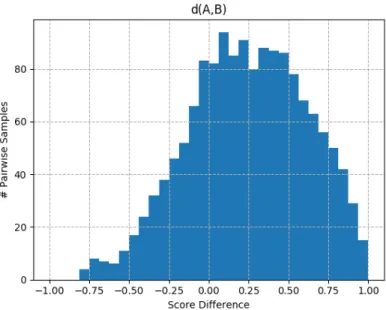
Once clusters are formed, for every pair of clusters, an empirical distribution of cross-cluster score differences is computed. This is done by taking every cross-cross-cluster pair of teams that has competed against each other, computing their score differences, and aggregating the results. Such an empirical distribution for two clusters A and B, d(A, B), is shown in Fig 2-6. If this distribution has more than 50 samples then a predictor statistic is calculated using equation 2.21. A pseudocode procedure for this entire process is detailed in Algorithm 1.
Predictor(d(A, B)) = E[d(A, B)]
σ(d(A, B)) (2.21)
The sign of this predictor statistic signals which of the two clusters will perform better and the magnitude gives a confidence of this prediction. For example, a
zero-Figure 2-6: Histogram of an example empirical cross-cluster score distribution. The x-axis is the score difference between a team in cluster A and a team in cluster B.
mean Gaussian indicates a perfectly balanced cluster match-up and would provide no predictive information. For contrast the distribution in Fig 2-6 has a predictor statistic of 0.65 and distributions with a predictor close to 1.5 have nearly all their weight on one of the clusters. These predictor statistics are then aggregated over all cluster pairs with over 50 samples.
2.3.2
Clustering Significance Testing
An important step in this process is significance testing. Significance testing in this context refers to the process of determining if the clustering results are significantly difficult than a random clustering selection. Here the significance of clusters is as-sessed by using the KS test to compare the empirical distribution of predictor statistics against a randomly generated predictor statistic distribution. In order to generate the random distribution, the leaderboard of every competition is scrambled – thus removing any correlation between team history or competence and performance but preserving overall network structure and clustering – then the steps of finding the predictor statistic distribution are repeated as outlined in Alg 1 except using the
Algorithm 1 Cross-Cluster Statistics
1: procedure genPredictorDistribution 2: cluster pairs ← all pairs of clusters
3: for pair in cluster pairs do
4: clustA ← first cluster in pair
5: clustB ← second cluster in pair
6: for teamA in clustA.teams() do
7: for teamB in clustB.teams() do
8: if teamA.competition() == teamB.competition() then
9: score diff ← teamA.score() − teamB.score()
10: d(clustA,clustB).append(score diff)
11: num samples ← length of d(clustA,clustB)
12: if num samples > 50 then
13: mean ← E[d(clustA,clustB)]
14: stddev ← σ(d(clustA,clustB))
15: predictor stat(clustA,clustB) ← mean/stddev
16: else
17: predictor stat(clustA,clustB) ← None return d, predictor stat
new scrambled team scores in place of the empirical scores. This randomization and comparison is repeated thousands of times for statistical purposes.
2.4
Holdout Prediction Testing
2.4.1
Partial Holdout
In order to test the predictive power of the various community detection methods, I perform partial holdout testing in which, during the computation of predictor statis-tics, I holdout or remove 5% of the team scores and the associated matchups from every competition. The the empirical distributions and predictor statistics are com-puted for all cluster pairs using no score information from the held out teams. For every held out team, I compare their relative performance to their predicted relative performance, as indicated by the predictor statistic between the cluster to which the held out team belongs and the cluster to which their competitor belongs. I aggregate these results over 500 trials to get an average sense of the predictive power. These steps are detailed in pseudocode in Alg 2.
Algorithm 2 Holdout Testing
1: procedure partialHoldout 2: stats ← [0, 0, 0, 0]
3: competitions ← list of competitions
4: i ← 0
5: while i < 500 do
6: for comp in competitions do
7: n ← length of comp.teams()
8: heldout teams ← random ceil(0.05n) teams from comp.teams()
9: heldin teams ← the left over floor(0.95n) teams from comp.teams()
10: heldout matchups ← all the (unique) match ups of heldout teams
11: stats + = holdoutStatistics(heldin teams,heldout matchups)
12: i+ = 1
return stats
13: procedure wholeCompetitionHoldout 14: stats ← [0, 0, 0, 0]
15: competitions ← list of competitions
16: for heldout comp in competitions do
17: for comp in competitions do
18: if heldout comp == comp then
19: heldout teams ← comp.teams()
20: heldout matchups ← all the (unique) match ups of heldout teams
21: else
22: heldin teams ← comp.teams()
23: stats + = holdoutStatistics(heldin teams,heldout matchups) return stats
24: procedure holdoutStatistics(heldin teams, heldout matchups) 25: predictor stat ← genPredictorDistribution() using heldin teams
26: [same cluster,stat weak,correct prediction,incorrect prediction] ← [0, 0, 0, 0]
27: for matchup in heldout matchups do
28: clustA ← cluster of first team in matchup
29: clustB ← cluster ofsecond team in matchup
30: if clustA == clustB then
31: same cluster + = 1
32: else if predictor stat == None then
33: stat weak + = 1
34: else if sign(matchup.score diff()) == sign(predictor stat(clustA,clustB)) then
35: correct prediction + = 1
36: else
37: incorrect prediciton + = 1
2.4.2
Whole Competition Holdout
The above partial holdout is a first step but the ideal performance metric is whether or not these methods can predict the performance of teams without knowing any of the results from the competition in which the teams are competing. In a real world scenario, this corresponds to seeing all of the Kaggle teams in a competition and predicting the final leaderboard standings. Another real world example would be being given the NCAA season rosters and making a march madness bracket. In reality my methodology is slightly different since I only look at pairwise relative performance thus my predictions are not bound by transitivity (e.g. the idea that if A beats B and if B beats C, then A must beat C).
The methodology for whole competition holdout is very similar to partial holdout and is also detailed in Alg 2. In words, the procedure is to hold out a competition then compute the predictor statistics between cluster pairs using score data from all other competitions. Then, using the matchups from the heldout competition, the accuracy of the predictor statistics is assessed by making predictions on the heldout matchups. This process is repeated for all competitions and the results are aggregated to give an average sense of the predictive power of each method. With both of these methodologies, the prediction systems still have access to future information for the sake of simplicity.
Chapter 3
Results
3.1
Clustering Results
3.1.1
Optimal Number of Clusters
The first set of results is the optimal number of clusters for spectral clustering of the various projection methods as determined by the two cluster indices. For each of the two Kaggle preprocessing methods there are four projection methods for which the optimal number of clusters need to be found. All of the following plots show a similar format, number of clusters is displayed on the x-axis with a range from 10 to 500 clusters with a resolution of 10 clusters; the y-axis displays the value of the given cluster index. For the baseline projection method only the Davies-Bouldin index could be used due to the memory constraints of having a higher dimensionality caused by clustering all node types instead of only team node types.
The clustering indices as shown in Figure 3-1 show very clear trends and there is very little difference across preprocessing versions. Interestingly, baseline, unweighted and cosine similarity all show similar behavior in that the Davies-Bouldin Index starts off (generally) large before dropping and then spiking up when the C Index reaches its minimum or elbow. This correlated behavior is odd given that for both indices lower is better, meaning Davies-Bouldin gets worse when C Index gets better. The trends of the unweighted and cosine similarity methods let us also reasonably infer
what the C Index would look like for Baseline.
The SimRank based method shows considerably different behaviour than the other 3 methods in that the Davies-Bouldin index achieves a unique global maximum at the inflection point of the C Index, whose trend continues downward for all the cluster quantities tried. Here the elbow method must be applied to the C index trend since it is continuously decreasing, and again there is correlated behaviour between the two indices yet no consensus on what is the best clustering.
For the remainder of the results I consider the clusters:
Version 1 Baseline Unweighted Cosine SimRank
Num Clusters 390 100 80 100
Version 2 Baseline Unweighted Cosine SimRank
Num Clusters 380 170 150 110
Table 3.1: ’Optimal’ number of clusters for each method
Given that these cluster optimality indices have no guarantee to correlate with the holdout performance task, the clustering that results in the large correlated events seen above is chosen as ’optimal’ and the relationship between clustering and holdout performance will be examined later in a limited case in order to validate whether or not these clustering indices are a useful way to pick clusterings.
3.1.2
Cluster Size Distribution
Figure 3-2 shows the size distributions of the resultant clusterings from table 3.1. One can see that the baseline method yields a disproportionate number of singleton clusters, i.e. clusters with only one team. Singleton clusters in version 1 are essentially useless because, when they are held out, no data about their potential performance is available. In version 2 this is less of a problem but it is still detrimental, especially when a team has competed in only one or a small number of competitions. All methods, other than SimRank produce at least one singleton cluster.
3.1.3
Cluster Significance
Figures 3-3 and 3-4 show the p-values and D-statistics respectively returned by the KS-test for randomized significance testing. One can see that version 1 of Unweighted and Cosine Similarity have the lowest p-values and border on insignificantly different from random. Both versions of SimRank have the most significant results from the KS-test. Version 1 of Unweighted and Cosine Similarity also have the highest variance of any D-statistic distribution. The mean D-statistic varies greatly between versions and methods however SimRank achieves the largest mean when controlling for version.
3.2
Holdout Testing
3.2.1
Partial Holdout Testing
The results for partial holdout testing can be found tabulated in Tables 3.2 and 3.3 for preprocessing versions 1 and 2 respectively.
The category ’N’ is the number of heldout matchups aggregated over the 500 trials. The variation in ’N’ is due to the differing numbers of teams thrown out in the cluster preprocessing step and the fact that only 5% of non thrown out teams are held out from each competition. ’Same Cluster’ is the amount of matchups that occurred between two teams within the same cluster. When two teams are placed into the same cluster their relative performance cannot be predicted with this methodology, thus lower is generally better. ’Statistically Weak’ corresponds to the number of matchups that occurred between two clusters that did not meet the threshold of statistical power and thus can not be guessed on, lower is better. ’Correct’ and ’Incorrect’ are the total fraction of matchups that were predicted correctly and incorrectly respectively. ’Accuracy’ is the fraction of correctly guessed matchups out of all matchups able to be predicted. ’Adjusted Accuracy’ is the Accuracy that would be achieved if a mixed prediction strategy was used, wherein any matchup that could not be predicted in the above framework was determined with a 50/50 coin flip.
much better across the board when one considers Adjusted Accuracy. This is due to the fact that a far larger number of samples is guessed on in version 2 over version 1. For Unweighted and Cosine Similarity, the base Accuracy also increases. Interestingly version 1 of Baseline has an incredible base Accuracy but can only guess on a small number of samples. This suggests that, while only a few valid partitions exist they are incredibly close to reality.
Baseline Unweighted Cosine SimRank
N 1.52e9 1.51e9 1.51e9 1.47e9
Same Cluster 94.70% 77.94% 78.50% 46.64% Statistically Weak 0.65% 0.01% 0.01% 0.39% Correct 3.35% 12.11% 11.85% 33.78% Incorrect 1.14% 9.94% 9.65% 19.18% Accuracy 75.52% 54.91% 55.12% 63.78% Adjusted Accuracy 51.18% 51.08% 51.10% 57.30%
Table 3.2: Details of partial holdout prediction testing for the version 1 projection methods. All figures except for Accuracy are given as a percentage of N .
Baseline Unweighted Cosine SimRank
N 3.41e9 3.19e9 3.19e9 3.41e9
Same Cluster 51.38% 28.24% 32.20% 39.77% Statistically Weak 0.22% 0.17% 0.15% 0.16% Correct 30.99% 43.53% 41.99% 38.24% Incorrect 17.41% 28.06% 25.67% 21.83% Accuracy 64.03% 60.80% 62.06% 63.66% Adjusted Accuracy 56.79% 57.73% 58.16% 58.20%
Table 3.3: Details of partial holdout prediction testing for the version 2 projection methods. All figures except for Accuracy are given as a percentage of N .
Figure 3-5 plots the partial holdout prediction accuracy (blue) and sample size (orange) binned by prediction confidence as measured by the magnitude of the Pre-dictor statistic. This allows us to see if there is any statistical correlation between the magnitude of the Predictor statistic and Accuracy, which would allow us to put more faith in certain predictions. As one can see, for nearly every case there is a strong correlation between confidence and accuracy. This relationship is strongest for low confidence where the number of samples is largest and most consistent. For regimes where the sample size drops precipitously, this trend is less striking and at times erratic. An illustrative example of this dependence on number of samples is Cosine Similarity (v1), where Accuracy solidly correlates with Confidence for the first five bins but then Accuracy drops as Samples does, before rebounding to form an almost
bi-modal overall trend.
3.2.2
Whole Competition Holdout
Whole Competition holdout is a much more difficult task and the results of the above section do not directly translate. The statistics are the same as above and versions 1 and 2 are depicted in Tables 3.4 and 3.5 respectively.
Here again version 2 vastly outperforms version 1. Baseline gives a much weaker performance than all the other methods and compared to its performance in partial holdout testing. Among version 1, SimRank is the only method that has remotely viable results, with Accuracy close to that of its version 2 counterpart and only falling short on the number of matchups it was able to guess. Unweighted fails spectacularly, performing even worse than a pure coin flip. Among version 2, Unweighted and Cosine Similarity give SimRank a run for the money with Cosine Similarity outperforming SimRank in Adjusted Accuracy since it was able to guess on a much higher proportion of the heldout matchups with nearly the same base accuracy.
Baseline Unweighted Cosine SimRank
N 3.09e7 3.08e7 3.08e7 3.00e7
Same Cluster 94.72% 77.95% 78.50% 46.51% Statistically Weak 4.89% 19.37% 17.99% 1.78% Correct 0.20% 1.12% 1.86% 31.62% Incorrect 0.19% 1.55% 1.66% 20.10% Accuracy 50.88% 41.98% 52.78% 61.14% Adjusted Accuracy 50.00% 49.79% 50.10% 55.76%
Table 3.4: Details of complete holdout prediction testing for the version 1 projection methods. All figures except for Accuracy are given as a percentage of N .
Baseline Unweighted Cosine SimRank
N 6.95e7 6.49e7 6.49e7 6.95e7
Same Cluster 51.37% 28.24% 32.16% 39.65% Statistically Weak 35.52% 1.34% 1.51% 2.56% Correct 6.85% 41.39% 40.48% 35.58% Incorrect 6.26% 29.03% 25.85% 22.21% Accuracy 52.24% 58.77% 61.03% 61.57% Adjusted Accuracy 50.29% 56.18% 57.31% 56.69%
Table 3.5: Details of complete holdout prediction testing for the version 2 projection methods. All figures except for Accuracy are given as a percentage of N .
Figure 3-6 shows a similar picture as figure 3-5, except here the results are for Complete Holdout rather than simply Partial Holdout. For these results, a correlation
between confidence and is much more tenuous, perhaps do to the drastically smaller number of samples generated by this testing methodology. For version 1 methods, so few samples are actually guessed on and performance is so poor that it would be foolish to search for a statistical correlation of confidence and accuracy in these results. For version 2 methods this is somewhat more reasonable and a positive correlation can be observed in the unweighted and cosine similarity methods when confidence is low and samples are high; however, as the number of samples drops the trend of accuracy becomes erratic and any correlation is destroyed. The SimRank method shows interesting behavior in this test as its Accuracy remains essentially constant with confidence while the number of samples is large.
Finally, in order to verify the ’optimality’ from section 3.1, I perform Complete Holdout Testing for increments of 50 clusters and plot the corresponding trends. This analysis is only done for version 2 of Cosine Similarity and SimRank since these are the highest scoring methods. The results depicted in Figure 3-7 show four trends in clockwise order: The percentage of unguessable matchups, which corresponds to ’Same Cluster’ + ’Statistically Weak’ from the above tables; ’Correct’;’Accuracy’; and ’Adjusted Accuracy’. From the ’Adjusted Accuracy’ trend one can see that the behavior of the C Index and Davies-Bouldin Index are well suited to identifying the optimal performance along this criteria. One can also see that SimRank is much more insensitive to the number of clusters than Cosine Similarity for all trends but that Cosine Similarity ultimately performs better than SimRank in the best case.
Figure 3-7: Trend of complete holdout results with number of clusters for Cosine Similarity and SimRank
Chapter 4
Discussion
As seen in the last section, the hypothesis of this thesis is confirmed by the results – the Kaggle network structure provides information about team performance and is capable of making predictions on unseen data. Furthermore, the results of this thesis show that a projection method such as Cosine Similarity is essential in order for good results and that Baseline clustering is inadequate for predicting the results of a competition.
A possible explanation for why projecting onto the team similarity graph yields better results is as follows: In the raw network, no teams are directly connected thus forcing spectral clustering to find clusters in a circuitous fashion through their intermediate connections with users and competitions. A projection method removes this somewhat extraneous information and makes the relationship between teams more explicit and making it easier to properly identify their communities.
While Spectral Clustering provided good results even before any tuning or op-timization took place, DBSCAN was not nearly as well suited for the task. For all configurations attempted, DBSCAN found virtually useless clusterings – often finding a unique cluster for nearly every team. This behaviour is undesirable for a number of reasons, not least of which is extremely high dimensionality which prohibits further analysis due to computational constraints. DBSCAN’s failure is most-likely due to the high dimensionality of the data and correspondingly sparse (in the distance sense) distribution. Since DBSCAN looks for clusters of high density, these properties of the
data likely fool DBSCAN into classifying every data point as an island, far far away from every other datapoint. The dimensionality and sparseness of the data are a bad fit for DBSCAN but are easily overcome by spectral clustering, which can effectively reduce the dimensionality of the data by only considering the top k eigenvectors and defeats sparsity by forcing the data into a predefined number of clusters, thereby precluding the outcome where every datapoint is an island onto itself.
Another finding of this thesis is that both the C Index and the Davies-Bouldin Index strongly correlate with the performance in the competition holdout task. How-ever, it is very surprising that performance is anti-correlated with the Davies-Bouldin Index which seeks to simultaneously minimize the distance of cluster points to their cluster centers and maximize the distance between cluster centers. It is even more surprising given that performance is positively correlated with the C Index which at-tempts to minimize the set of intra-cluster distances relative to all pairs of distances present in the current clustering. It is unclear at present why the correlations with these two indices differ in sign, or why these metrics fundamentally correlate with performance in the competition holdout task in the first place.
Surprisingly, Cosine Similarity outperforms SimRank when paired with the ver-sion 2 processing that allows for non-unique teams. This is not intuitively obvious, since SimRank provides slightly more information than Cosine Similarity but it might suggest that only first order interactions in the Kaggle network, i.e. how many team-mates two teams share, is import for finding performance correlated communities. However, the performance of SimRank is very robust to both preprocessing and num-ber of clusters chosen, making it a reasonable choice for an unexplored or unoptimized system.
It is reasonable that these methods can be directly applied to the prediction of sports performance. Instead of the Competition-Team-User network, one can use the World Cup-Team-Athlete network or similar for the sport of choice. In each sport there is a well-defined notion of score that is persistent so the use of a normalized score would be unnecessary. Given the nature of sports tournaments, the cut-offs for statistical significance would also have to be readjusted.
For application to a corporate or research setting, more work would be required. Conveniently, these methods do not require performance information upfront and communities can be found using only structural information. Since performance is harder to numerically quantify in these domains, it is likely that human intervention would be needed in order to use available performance information to compare clusters and rule which cluster would be better suited for a task.
This work is only a first pass at investigating this problem as the full parameter space was not fully explored so the results are likely suboptimal – this is especially true for Cosine Similarity and SimRank where there are 2 and 3 unique parameters to tune respectively. Exploring this parameter space and tuning it presents an interesting challenge in and of itself and it is unclear whether or not this dataset is big enough for traditional Train-Validate-Test methodologies. A larger dataset would also afford the more traditional Train-Test split of data; the methodology in this work is similar but it is non-traditional and non-causal, i.e. the first competitions are predicted using data from the last competitions. It is unclear at present if causal prediction would fair better or worse than non-causal prediction. Another axis in which these methods should be compared is how often competing teams are placed in the same cluster and what can be said about their relative performance given that they are in the same cluster. Lastly, although I hypothesize that these methods are general, these results must be repeated on a dataset from a different domain to confirm their generality.
Bibliography
[1] R´eka Albert and Albert-L´aszl´o Barab´asi. Statistical mechanics of complex net-works. Rev. Mod. Phys., 74:47–97, Jan 2002.
[2] S. Boccaletti, V. Latora, Y. Moreno, M. Chavez, and D.-U. Hwang. Complex networks: Structure and dynamics. Physics Reports, 424(4):175 – 308, 2006. [3] John S. Breese, David Heckerman, and Carl Kadie. Empirical analysis of
pre-dictive algorithms for collaborative filtering. In Proceedings of the Fourteenth Conference on Uncertainty in Artificial Intelligence, UAI’98, pages 43–52, San Francisco, CA, USA, 1998. Morgan Kaufmann Publishers Inc.
[4] T. Caliski and J Harabasz. A dendrite method for cluster analysis. Communi-cations in Statistics, 3(1):1–27, 1974.
[5] Shihyen Chen, Bin Ma, and Kaizhong Zhang. On the similarity metric and the distance metric. Theoretical Computer Science, 410(24):2365 – 2376, 2009. Formal Languages and Applications: A Collection of Papers in Honor of Sheng Yu.
[6] D. L. Davies and D. W. Bouldin. A cluster separation measure. IEEE Transac-tions on Pattern Analysis and Machine Intelligence, PAMI-1(2):224–227, April 1979.
[7] Bernard Desgraupes. Clustering indices. 2017.
[8] Martin Ester, Hans-Peter Kriegel, Jrg Sander, and Xiaowei Xu. A density-based algorithm for discovering clusters in large spatial databases with noise. pages 226–231. AAAI Press, 1996.
[9] Roger Guimer`a, Brian Uzzi, Jarrett Spiro, and Lu´ıs A. Nunes Amaral. Team assembly mechanisms determine collaboration network structure and team per-formance. Science, 308(5722):697–702, 2005.
[10] Lawrence Hubert and James Schultz. Quadratic assignment as a general data analysis strategy. British Journal of Mathematical and Statistical Psychology, 29(2):190–241.
[12] Kaggle Inc. Kaggle platform, 2018.
[13] Glen Jeh and Jennifer Widom. Simrank: A measure of structural-context sim-ilarity. In Proceedings of the Eighth ACM SIGKDD International Conference on Knowledge Discovery and Data Mining, KDD ’02, pages 538–543, New York, NY, USA, 2002. ACM.
[14] Eric Jones, Travis Oliphant, Pearu Peterson, et al. SciPy: Open source scientific tools for Python, 2001–. [Online; accessed ¡today¿].
[15] G. Linden, B. Smith, and J. York. Amazon.com recommendations: Item-to-item collaborative filtering. IEEE Internet Computing, 7:76–80, 01 2003.
[16] S. Lloyd. Least squares quantization in pcm. page 129137, 1982.
[17] Wes McKinney. Data structures for statistical computing in python. In St´efan van der Walt and Jarrod Millman, editors, Proceedings of the 9th Python in Science Conference, pages 51 – 56, 2010.
[18] M. E. J. Newman. The structure of scientific collaboration networks. Proceedings of the National Academy of Sciences, 98(2):404–409, 2001.
[19] F. Pedregosa, G. Varoquaux, A. Gramfort, V. Michel, B. Thirion, O. Grisel, M. Blondel, P. Prettenhofer, R. Weiss, V. Dubourg, J. Vanderplas, A. Passos, D. Cournapeau, M. Brucher, M. Perrot, and E. Duchesnay. Scikit-learn: Machine learning in Python. Journal of Machine Learning Research, 12:2825–2830, 2011. [20] Jos´e J. Ramasco, S. N. Dorogovtsev, and Romualdo Pastor-Satorras.
Self-organization of collaboration networks. Phys. Rev. E, 70:036106, Sep 2004. [21] Peter J. Rousseeuw. Silhouettes: A graphical aid to the interpretation and
vali-dation of cluster analysis. Journal of Computational and Applied Mathematics, 20:53 – 65, 1987.
[22] Gerard Salton. Automatic Text Processing: The Transformation, Analysis, and Retrieval of Information by Computer. Addison-Wesley Longman Publishing Co., Inc., Boston, MA, USA, 1989.
[23] Badrul Sarwar, George Karypis, Joseph Konstan, and John Riedl. Item-based collaborative filtering recommendation algorithms. In Proceedings of the 10th International Conference on World Wide Web, WWW ’01, pages 285–295, New York, NY, USA, 2001. ACM.
[24] Daniel A. Schult. Exploring network structure, dynamics, and function using networkx. In In Proceedings of the 7th Python in Science Conference (SciPy, pages 11–15, 2008.
[25] Raymond T. Sparrowe, Robert C. Liden, Sandy J. Wayne, and Maria L. Kraimer. Social networks and the performance of individuals and groups. Academy of Management Journal, 44(2):316–325, 2001.
[26] H. Steinhaus. Sur la division des corp materiels en parties. page 801804, 1956. [27] Ulrike von Luxburg. A tutorial on spectral clustering. CoRR, abs/0711.0189,