HAL Id: hal-00553818
https://hal.archives-ouvertes.fr/hal-00553818
Submitted on 9 Jan 2011HAL is a multi-disciplinary open access archive for the deposit and dissemination of sci-entific research documents, whether they are pub-lished or not. The documents may come from teaching and research institutions in France or abroad, or from public or private research centers.
L’archive ouverte pluridisciplinaire HAL, est destinée au dépôt et à la diffusion de documents scientifiques de niveau recherche, publiés ou non, émanant des établissements d’enseignement et de recherche français ou étrangers, des laboratoires publics ou privés.
Julien Cristau
To cite this version:
Julien Cristau. Automata and temporal logic over arbitrary linear time. Foundations of Soft-ware Technology and Theoretical Computer Science, Dec 2009, Kanpur, India. pp.133-144, �10.4230/LIPIcs.FSTTCS.2009.2313�. �hal-00553818�
Automata and temporal logic over
arbitrary linear time
Julien Cristau
LIAFA — CNRS & Universit´e Paris 7 ABSTRACT. Linear temporal logic was introduced in order to reason about reactive systems. It is often considered with respect to infinite words, to specify the behaviour of long-running systems. One can consider more general models for linear time, using words indexed by arbitrary linear orderings. We investigate the connections between temporal logic and automata on linear orderings, as introduced by Bruy`ere and Carton. We provide a doubly exponential procedure to compute from any LTL formula with Until, Since, and the Stavi connectives an automaton that decides whether that formula holds on the input word. In particular, since the emptiness problem for these automata is decidable, this transformation gives a decision procedure for the satisfiability of the logic.
1
Introduction
Temporal logic, in particular LTL, was proposed by Pnueli to specify the behaviour of re-active systems [12]. The model of time usually considered is the ordered set of natural numbers, and executions of the system are seen as infinite words on some set of atomic propositions. This logic was shown to have the same expressive power as the first order logic of order [11], but it provides a more convenient formalism to express verification prop-erties. It is also more tractable: while the satisfiability problem of FO is non-elementary [18], it was shown in [17] that the decision problem of LTL with Until and Since on ω-words is PSPACE-complete. This logic has also strong ties with automata, with important work to provide efficient translations to B ¨uchi automata, e.g. [10].
Within this time model, a number of extensions of the logic and the automata model have been studied. But one can also consider more general models of time: general linear time could be useful in different settings, including concurrency, asynchronous communi-cation, and others, where using the set of integers can be too simplistic. Possible choices include ordinals, the reals, or even arbitrary linear orderings. In terms of expressivity, while LTL with Until and Since is expressively complete (i.e. equivalent to FO) on Dedekind-complete orderings (which includes the ordering of the reals as well as all ordinals), this does not hold in the general case. Two more connectives, the future and past Stavi opera-tors, are necessary to handle gaps [9] when considering arbitrary linear orderings.
Over ordinals, LTL with Until and Since has been shown to have a PSPACE-complete satisfiability problem [7]. Over the ordering of the real numbers, satisfiability of LTL with until and since is PSPACE-complete, but satisfiability of MSO is undecidable. Over general linear time, first order logic has been shown to be decidable, as well as universal monadic second order logic. Reynolds shows in [13] that the satisfiability problem of temporal logic with only the Until connective is also PSPACE-complete, and conjectures that this might stay
true when adding the Since connective. The upper bound in [7] is obtained by reducing the satisfiability of LTL formulae to the accessibility problem in an appropriate automata model,
c
accepting words indexed by ordinals. In this paper, we focus on the general case of arbitrary linear orderings, using the full logic with Until, Since and both Stavi connectives. Our aim is to investigate the connections between LTL and automata in this setting.
Automata on linear orderings were introduced by Bruy`ere and Carton [3]. This model extends traditional finite automata using “limit” transitions to handle positions with no suc-cessor or predesuc-cessor, furthering B ¨uchi’s model of automata on words of ordinal length [4]. Carton showed in [5] that accessibility over scattered ordering is decidable in polynomial time, and in [14] it was shown that these automata can be complemented over countable scattered linear orderings. The accessibility result can be extended to arbitrary orderings [6]. From any formula in this logic, we define an automaton which determines whether the formula holds on its input word. Satisfiability of the formula is reduced to accessibility in this automaton, and that way we get decidability of the satisfiability problem of LTL with Until, Since and the Stavi operators for any rational subclass.
Section 2 presents some definitions about linear orderings, linear temporal logic, and the model of automata used. Section 3 introduces our main result, an algorithm to translate any LTL formula into a corresponding automaton. Section 4 discusses the expressivity of the logic and automata considered, and looks at some natural fragments.
2
Definitions
2.1 Linear orderings
We first recall some basic definitions about orderings, and introduce some notations. For a complete introduction to linear orderings, the reader is referred to [15]. A linear ordering J is a totally ordered set(J,<)(considered modulo isomorphism). The sets of integers (ω), of
rational numbers (η), and of real numbers with the usual orderings are all linear orderings. Let J and K be two linear orderings. One defines the reversed ordering−J as the
order-ing obtained by reversorder-ing the relation<in J, and the ordering J+K as the disjoint union J⊔K extended with j < k for any j ∈ J and k ∈ K. For example, −ω is the ordering of
negative integers.−ω+ωis the usual ordering of Z, also denoted by ζ.
A non-empty subset K of an ordering J is an interval if for any i < j< k in J, if i∈K and k∈ K then j∈ K. In order to define the runs of an automaton, we use the notion of cut. A cut
of an ordering J is a partition(K, L)of J such that for any k∈K and l ∈L, k< l. We denote
by ˆJ the set of cuts of J. This set is equipped with the order defined by(K1, L1) < (K2, L2) if K1 ( K2. This ordering can be extended to J∪ ˆJ in a natural way ((K, L) < j iff j ∈ L). Notice that ˆJ always has a smallest and a biggest element, respectively cmin = (∅, J) and
cmax = (J, ∅). For example, the set of cuts of the finite ordering {0, 1, . . . , n−1} is the ordering{0, 1, . . . , n}, and the set of cuts of ω is ω+1.
For any element j of J, there are two successive cuts c−j and c+j , respectively ({i ∈ J | i< j},{i ∈ J | j≤ i})and({i∈ J |i≤ j},{i ∈ J | j< i}). A gap in an ordering J is a cut c
which is not an extremity (cmaxor cmin), and has neither a successor nor a predecessor. Given an alphabet Σ, a word of length J is a sequence(aj)j∈J of elements of Σ indexed by J. For example,(ab)ω is a word of length ω; the sequence abωabωa is a word of length
2.2 Temporal logic
We use words over linear orderings to model the behaviour of systems over linear time. To express properties of these systems, we consider linear temporal logic. The set of LTL formulae is defined by the following grammar, where p ranges over a set AP of atomic propositions: ϕ::= p| ¬ϕ| ϕ∨ϕ|ϕUϕ| ϕSϕ| ϕU′ϕ|ϕS′ϕ
Besides the usual boolean operators, we have four temporal connectives. TheU connec-tive is called “Until”, andS is called “Since”.U′andS′ are respectively the future and past Stavi connectives. Other usual connectives such as “Next” (X), “Eventually” (F), “Always” (G) can be defined using these, as we see below.
These formulae are interpreted on words over the alphabet 2AP. A letter in those words is the set of atomic propositions that hold at the corresponding position. Let x = (xj)j∈J a word of length J. A formula ϕ is evaluated at a particular position i in x; we say that ϕ holds at position i in x, and we write x, i|= ϕ, using the following semantics:
x, i|= p if p∈xi
x, i|= ¬ψ if x, i6|=ψ
x, i|=ψ1∨ψ2 if x, i|=ψ1or x, i|=ψ2
x, i|=ψ1Uψ2 if there exists j>i such that x, j|= ψ2,
and for any k such that i<k< j, we have x, k|=ψ1 x, i|=ψ1Sψ2 if −x, i|=ψ1Uψ2where−x is the reversed word(aj)j∈−J
x, i|= ψ1U′ψ2 if there exists a gap c∈ ˆJ verifying three properties: (1) x, j|=ψ1for any position j such that i <j<c
(2) there is no interval starting at c where ψ1is always true (i.e.∀c<k∃c< j<k x, j|= ¬ψ1), and
(3) ψ2is always true in some interval starting at c
x, i|= ψ1S′ψ2 if −x, i|=ψ1U′ψ2(it is the corresponding past connective)
Note that we use a “strict” semantic for the Until operator, contrary to a common defi-nition, which would be:
x, i|=ψ1Unsψ2 if there exists j≥i such that x, j |=ψ2and x, k|= ψ1for any i≤ k< j. In the strict version, the current position i is not considered for either the ψ1or the ψ2part of the definition. Using the strict or non-strict version makes no difference when considering
ω-words, but in the case of arbitrary orderings, the strict Until is more powerful, as noted by Reynolds in [13].
The formula “Next ϕ”, or X ϕ, is equivalent to ⊥Uϕ. “Eventually ϕ”, noted F ϕ, is
ϕ∨ (⊤Uϕ), and “always ϕ”, notedGϕ, can be expressed as¬(F (¬ϕ)).
Given a word x of length J, the truth word of ϕ on x is the word vϕ(x)of length J over the alphabet{0, 1}where the position j is labelled by 1 iff x, j |= ϕ. A formula is valid if its truth word on any input only has ones. A formula is satisfiable if there exists an input word such that the truth word contains a one.
Consider the formula ϕ= ¬a∧ (G ¬ X a), with AP= {a}. If x= (a∅)ω(where a stands for{a}), then vϕ(x) =0ω(at every position, either a is true or a is true in the successor). On the other hand, if x = a∅ωa∅ωa, then v
ϕ(x) = 01ω01ω0: at positions 0, ω and at the last position, a is true so the formula doesn’t hold; at all other positions, a is false, and there is no position in the input word whereX a holds.
The satisfiability problem for a formula ϕ consists in deciding whether there exists a word
w and a position i in w such that w, i |= ϕ. As FO is decidable, and every LTL formula can be expressed using first order, satisfiability of LTL is decidable. Note however that in terms of complexity FO is already non-elementary on finite words [18], which is not true of LTL.
2.3 Automata
On infinite words, B ¨uchi automata can be used to decide satisfiability of LTL formulae. In the case of words over linear orderings, a model of automata has been introduced in [3]. Instead of accepting or rejecting each input word, as in the case of ω-words, we use these automata to compute the truth words corresponding to an LTL formula. Our model of automata thus has an output letter on each transition, so they are actually letter-to-letter transducers, which make composition easier (see Section 3.1).
An automaton is a tuple A = (Q, Σ, Γ, δ, I, F) where Q is a finite set of states, Σ is a finite input alphabet, Γ is a finite output alphabet, I and F are subsets of Q, respectively the set of initial and final states, and δ ⊆ (Q×Σ×Γ×Q) ∪ (2Q×Q) ∪ (Q×2Q)is the set of transitions. We note:
• p−→a|b q if(p, a, b, q) ∈δ(successor transition) • P→q if(P, q) ∈δ(left limit transition) • q→ P if(q, P) ∈δ(right limit transition).
Consider a word x = (qj)j∈J over Q. We define the left and right limit sets of x at position j∈ J as the sets of labels that appear arbitrarily close to j (respectively to its left and
to its right). Formally:
limj−x= {q∈Q| ∀k< j∃i k <i<j∧qi = q}
limj+x= {q∈Q| ∀k> j∃i j <i< k∧qi = q}
Note that limj−x is non-empty if and only if the transition to j is a left limit, and similarly
for limj+x if the transition from j is a right limit. These sets help define the possible limit
transitions in a run.
Given an automaton A, an accepting run of Aon a word x = (xj)j∈J is a word ρ of length ˆJ over Q such that:
• ρcmin ∈ I and ρcmax ∈F;
• for each i∈ J, there exists yi ∈Γsuch that ρc−i xi|yi
−−→ρc+
i ;
• if c ∈ ˆJ has no predecessor, limc−ρ→ρc, and if c∈ ˆJ has no successor, ρc →limc+ρ.
EXAMPLE 1. The first automaton in Figure 1 outputs 1 at each position immediately fol-lowed by a 1 in the input word, and 0 at other positions.
The second automaton accepts input words whose length is a linear ordering without first or last element, and without two consecutive elements (i.e. dense orderings). The notation P→q0, q1means that there is a transition P→q0and a transition P →q1.
q0 q1 q2 −|1 −|0 1|1 1|0 0|1 0|0 Limits: P →q0 q0→ P q2→ P for any P ⊆ {q0, q1, q2} q0 q1 −|− q2 Limits: {q1, q2},{q0, q1, q2} →q0, q1 q1, q2 → {q1, q2},{q0, q1, q2} Figure 1: Example automata
In [5], Carton proves that the accessibility problem on these automata can be solved in polynomial time, when only considering scattered orderings. This result can be extended to arbitrary orderings [6] as it is done for rational expressions in [2]. The idea is to build an automaton over finite words which simulates the paths in the initial automaton and re-members their contents. In order to handle the general case (as opposed to only scattered orderings), the added operation is called “shuffle”: sh(w1, . . . , wn) = Πj∈Jxj where J is a dense and complete ordering without a first or last element, partitioned in dense subor-derings J1. . . Jn, such that xj = wi if j ∈ Ji. Looking at automata, this means that if there are paths from p1 to q1 with content P1, . . . , from pn to qn with content Pn, and transitions from P1∪ · · · ∪Pnto each pi, transitions from each qi to P1∪ · · · ∪Pn, a transition from p to
P1∪ · · · ∪Pnand a transition from P1∪ · · · ∪Pnto q, then there is a path from p to q.
3
Translation between formulae and automata
Over ω-words, problems on temporal logics are commonly solved using tableau meth-ods [20], or automata-based techniques [19]. In this work we extend the correspondence between LTL and automata to words over linear orderings. Our main result is Theorem 2.
THEOREM 2. For every LTL formula ϕ, there is an automaton Aϕ which given any input word x outputs the truth word vϕ(x).
Moreover, this automatonAϕ can be effectively computed, and has a number of states exponential in the size of ϕ. Because we can compute the product ofAϕwith any given au-tomaton and check for its emptiness, we get Corollary 3, which states that given a temporal formula and a rational property (i.e. an automaton on words over linear orderings), we can check whether there exists a model of the formula which is accepted by the automaton.
COROLLARY3. The satisfiability problem for any rational subclass is decidable.
The idea is to build Aϕ by induction on the formula. We construct an elementary au-tomaton for each logical connective. We use composition and product operations to build inductively the automaton of any LTL formula from elementary automata. All automata used in this proof have the particular property that there exists exactly one accepting run for each possible input word, i.e. they are non-deterministic, but also non-ambiguous. This property is preserved by composition and product.
The structure of the proof is the following: we define the composition and product op-erators on automata, then we present the elementary automata that are needed to encode logical connectives. Finally, we give the inductive method to build the automaton corre-sponding to a formula from elementary ones.
3.1 Product, composition and elementary automata
Let A1 = (Q1, Σ, Γ, δ1, I1, F1) and A2 = (Q2, Σ′, ∆, δ2, I2, F2) be two automata. The prod-uct consists in running both automata with the same input alphabet in parallel, and out-putting the combination of their outputs. IfA1’s output alphabet andA2’s input alphabet are the same, the composition consists in runningA2overA1’s output. We use the notation
π1(a, b) =a and π2(a, b) =b for the first and second projections.
DEFINITION 4. Suppose thatA1 andA2 have the same input alphabet, i.e. Σ = Σ′. The productof A1 andA2 is the automatonA1× A2 = (Q1×Q2, Σ, Γ×∆, δ, I1×I2, F1×F2), where δ contains the following transitions:
• (q1, q2) a|b,c −−→ (q′1, q′2)if q1 a|b −→q′1and q2 a|c −→q2′, • (q1, q2) →Pif q1→π1(P)and q2→π2(P), • P→ (q1, q2)if π1(P) →q1and π2(P) →q2.
DEFINITION5.Suppose now that the output alphabet ofA1is the input alphabet ofA2, i.e. Γ = Σ′. The composition of A1 andA2 is the automatonA2◦ A1 = (Q1×Q2, Σ, ∆, δ, I1×
I2, F1×F2). The transitions in δ are: • (q1, q2) a|c −→ (q′1, q2′)if q1 a|b −→q′1and q2 b|c −→q2′, • (q1, q2) →Pif q1→π1(P)and q2→π2(P), • P→ (q1, q2)if π1(P) →q1and π2(P) →q2.
Recall that LTL formulae are given by ϕ := p| ¬ϕ|ϕ∨ϕ| ϕUϕ|ϕU′ϕ|ϕSϕ| ϕS′ϕ. For each atomic proposition p we construct an automatonAp which, given a word x, out-puts vp(x). For each logical connective of arity n, we construct an automaton with input alphabet{0, 1}n, and output alphabet{0, 1}. The input word is the tuple of truth words of the connective’s variables, the output is the truth word of the complete formula. For tempo-ral connectives, we only describe the automata corresponding toU andU′. For the “past” connectives, the automata are the same with all transitions (successor and limits) reversed, and initial and final states swapped.
For any p ∈ AP, the automatonAp is({q}, 2AP,{0, 1}, δ,{q},{q}) where δ = {(q a|0 −→ q| p 6∈ a} ∪ {q −→a|1 q| p ∈ a} ∪ {q → {q},{q} → q}. This automaton simply outputs 1 at positions where p is true, and 0 everywhere else. Note that the run is uniquely determined by the input word; such a transducer is called non-ambiguous.
Figures 2(a) and 2(b) show the automata corresponding to the negation (¬) and dis-junction (∨) connectives. Their limit transitions are {q} → q and q → {q}. Again, these automata admit exactly one run for each input word.
q
0|1 1|0
(a) Automaton for negation
q
0, 0|0 0, 1|1 1, 0|1 1, 1|1
3.2 Automaton for
U
The difficulty starts with the “Until” connective (U). We recall that ϕUψholds at position i in a word w if there exists j>i such that ψ holds at j, and such that ϕ holds at every position k such that i<k < j.
We build an automaton AU with input alphabet {0, 1}2 (corresponding to the truth
value of ϕ and ψ at each position), and output alphabet {0, 1}. On an input word of the form(vϕ(w), vψ(w))for some word w, we want the output to be vϕUψ(w). Let J= |w|, and
c∈ ˆJ. We have five different situations. For each of these cases the figure shows an example,
with “|” representing the cut c, and each•representing a position in the input word. 0. c is followed by a position where ϕ and ψ are true. input
output · · · •1| 1,1
• · · ·
1. c= c−j , and j is such that ϕ is false and ψ is true. input
output · · · •1| 0,1
• · · ·
2. other cases where ϕUψis true at c. input
output · · · •1| 1,−
z}|{
· · · −• · · ·,1
3. c is followed by a position where both ϕ and ψ are false. input
output · · · •0| 0,0
• · · ·
4. other cases where ϕUψis false at c. If c=c−j then the input at position j is(1, 0).
input output · · · •0| 1,0 z}|{ · · · 0,0• · · · • 0| 1,0 z}|{ · · · {(1,−),(0,1)} z }| { · · · ·
The structure of the automatonAUand the limit transitions are given by Figure 2. This
automaton has five states q0 to q4 corresponding to the situations described above. Given any two states q and q′ there exists a transition q → q′ except from q2to q3 or q4 and from
q4to q0, q1 or q2. The input label of successor transitions is determined by the origin node: (1, 1) for q0, (0, 1) for q1, (0, 0) for q3, and (1, 0) for q2 and q4. The output label is 1 on transitions leading to q0, q1 or q2, and 0 on transitions leading to q3 or q4. All states are initial, while q4is the only final state.
LEMMA6. Let ϕ and ψ two formulae. Let x and y be the truth words of ϕ and ψ on a word
wof length J. The output ofAU on(x, y)is the truth word of ϕUψon w.
PROOF. Let ρ be the word of length ˆJ on Q defined by • if xj =yj =1, then ρ(c−j ) =q0;
• if xj =0 and yj =1 then ρ(c−j ) =q1; • if xj =yj =0 then ρ(c−j ) =q3;
• otherwise, if there exists j>c such that yj =1 and for all i such that c <i< j, xi =1,
then ρ(c) =q2; • otherwise, ρ(c) =q4.
We show that ρ is a run ofAU, that it is unique, and that its output is indeed the truth word
of ϕUψon w.
By definition, ρ ends in q4, which is the final state of AU. Let c ∈ ˆJ. If ρ(c)is q0, q1 or
q3, then c = c−j for some j and the successor transition from c to the next cut is allowed by the automaton. If ρ(c) = q2, and c= c−j for some j, then xj =1 and yj =0, and ρ(c+j )is q0,
q0 q1 q2 q3 q4 1, 1/1 0, 1/1 1, 0/1 0, 0/0 1, 0/0 1, 1/1 1, 1/0 0, 0/1 0, 1/1 0, 0/0 P → q0, q1, q2, q3, q4 if q0, q1or q3 ∈P {q2} → q0, q1, q2 {q4} → q3, q4 q2 → {q0},{q2},{q0, q2} q4 → P if q1or q3∈ P q4 → {q4}
Figure 2: Automaton forU
q1or q2. If ρ(c−j ) = q4, then similarly xj = 1 and yj = 0, and ρ(c+j )can be q3 or q4. Every successor transition in ρ is thus allowed byAU.
We now need to show the same for limit transitions. If a left limit transition leads to a cut c, then either ψ is true arbitrarily close to the left of c (in which case the corresponding limit set contains q0 or q1), or it is always false (and the limit set is {q2} or a subset of {q3, q4}). If the limit set contains q0, q1or q3, any state for c is allowed. If it is{q2}, the cut c can’t be labelled by q3or q4without violating the definition of ρ. Conversely, if the limit set is{q4}, ρ(c)is necessarily q3or q4.
Let’s now consider a right limit transition starting at a cut c. The label of this cut can only be q2 or q4. In the first case, ϕ must be true everywhere in the limit set, which is thus a subset of{q0, q2}. In the second case, either ϕ is false infinitely often in the limit, or ψ is always false. This means that the limit set contains q1or q3, or is restricted to{q4}.
We now show that a run onAU is uniquely determined by the input word. Let γ a run
ofAU on x, y. Because of the constraints on the successor transitions, a cut c is labelled by
q0, q1or q3in γ if and only if it is labelled by the same state in ρ.
Let’s suppose that a cut c is labelled by q2 in γ. Since q2is not final, there exists c′ > c labelled by some other state. If there is a first such cut, its label is necessarily q0or q1(by a successor transition from q2or a limit transition from{q2}). Otherwise, there is a transition of the form q2 → {q0}or q2 → {q0, q2}. In both cases, c satisfies the condition for cuts labelled by q2in the definition of ρ. A similar argument shows that a cut labelled by q4in γ has the same label in ρ. The run ofAUon a given input word is thus unique.
The last step is to show that the output word is really the truth word of ϕUψ. Let j an element of J. First, suppose that w, j|= ϕUψ. If j has a successor k, and ψ is true at k, then
yk =1, andAU outputs 1 at position j. Otherwise, there exists k> j such that w, k|= ψ(i.e.
yk = 1), and xℓ = 1 whenever j < ℓ < k. Thus, c+j is labelled with q2, andAU once again
outputs 1 at position j.
Similarly, if w, j 6|= ϕUψ, there are two cases. In the first case, j has a successor k, and
q2 q1 q0 q3 q7 q6 q5 q4 q 8 q9 1,1/0 0,1/0 1,0/0 0,0/0 1,0/1 1,1/1 • P→q0, q1, q2if P∩ {q4, q5} 6= ∅or P⊆ {q0, q1, q2} • P→q3if P⊆ {q0, q1, q2} • P → q4, q5, q6, q7 if P 6⊆ {q0, q1, q2} • P→q8if P∩ {q4, q5} 6=∅ • P → q9 if P∩ {q4, q5} = ∅ and P6⊆ {q0, q1, q2} • q0→ P if P⊆ {q0, q1, q2} • q3 → P if P∩ {q1, q4, q6} = ∅ and q5∈ P • q8→ P if P∩ {q4, q5, q6, q7} 6= ∅ • q9→ P if P∩ {q4, q5, q6, q7} 6= ∅and either P∩ {q4, q5} = ∅ or P intersects{q1, q4, q6} Figure 3: Automaton for the future Stavi operator
case, c+j is labelled by q4, and once againAU outputs 0.
3.3 Automaton for the future Stavi connective (
U
′)Let’s recall that ϕU′ψholds at position i if there exists a gap c >i such that ϕ holds at every
position i<j<c, the property ψ holds at every position in some interval starting at x, and ¬ϕholds at positions arbitrarily close to c to the right.
The central point in this definition is the gap c, which corresponds to state q3 in the automaton. States q0, q1 and q2 follow the positions, before q3, where the formula holds. States q4, q5, q6, q7, q8follow the positions where the formula doesn’t hold. If a run reaches
q0, q1 or q2, it has to leave this region through q3, and all successor transitions until then have input label(1, 0)or(1, 1). The structure of this automaton is depicted in Figure 3. All states except q3and q9are initial; q8and q9 are final. Transitions from q1and q7 have input label(1, 1), transitions from q2and q6have input label(1, 0), transitions from q4have input label(0, 0), and transitions from q5have input label(0, 1). The output is 1 for transitions to
q0, q1and q2, and 0 for transitions to q4, q5, q6, q7and q8.
We define a labelling ρ of the cuts of a word w on{0, 1}2using the states of the automa-ton in the following way:
• q0has no successor, ϕU′ψis true
• q1has an outgoing transition labelled(1, 0), ϕU′ψis true • q2has an outgoing transition labelled(1, 1), ϕU′ψis true • q3is a gap, ϕU′ψis true before it and false afterwards • q4has an outgoing transition labelled(0, 0), ϕU′ψis false • q5has an outgoing transition labelled(0, 1), ϕU′ψis false • q6has an outgoing transition labelled(1, 0), ϕU′ψis false • q7has an outgoing transition labelled(1, 1), ϕU′ψis false
• q8has no successor, ϕ doesn’t hold in the left limit if it has no predecessor, and ϕU′ψ is false
• q9is a gap or is the last cut, ϕU′ψis false, and ϕ is true in some interval to the left
LEMMA 7. ρ defines the unique run of the automaton on its input word. If the input is
(vϕ(w), vψ(w))for some word w, then the output of this run is vϕU′ψ(w).
PROOF. We first show that ρ is a run. Successor transitions correspond almost directly to
the definitions of the labelling ρ, so let’s look at limit transitions. For left limits, the following cases need to be considered:
• if a transition P→ q0is taken at a cut c, then either ϕ is true in the limit, and so ϕU′ψ is too, and P⊆ {q0, q1, q2}, or it’s not, and either q4or q5appear in the limit
• the same reasoning applies for q1and q2
• if c is labelled q3then the incoming transition has to come from a subset of{q0, q1, q2} since ϕU′ψis true in the limit.
• if a transition P → q4 is used, then ϕU′ψis not true in the limit (otherwise it would still be true), and so P6⊆ {q0, q1, q2}; the same applies for q5, q6, q7, q8and q9
• if c is a left limit and is labelled q8 then the incoming transition comes from a set P intersecting{q4, q5}because¬ϕis repeated
• if c is labelled q9then q4and q5can’t appear in the left limit set (ϕ is true)
If c is a right limit cut, it can only be labelled q0, q3, q8or q9. Here are the possible right-limit transitions:
• if a right-limit cut c is labelled q0, the limit transition has to go to a subset of{q0, q1, q2} since ϕU′ψholds in the limit
• if c is labelled with q3, the limit transition to its right leads necessarily to a set P not including q1, q4and q6since ψ is always true, and including q5because¬ϕis repeated • if c is labelled q8 or q9, the right limit set can’t be a subset of {q0, q1, q2}otherwise c
would have been labelled q0
• if c is labelled q9we have the additional condition that either ϕ holds in the limit (and neither q4nor q5appears) or ψ doesn’t (and one of q1, q4and q6is in the limit)
The labelling of cuts defined above is thus a path of the automaton, and we only need to show that it’s the only one, using the same method as for theAU. Moreover, the definition
of ρ means that the output is 1 whenever ϕU′ψholds, and 0 at all other positions.
3.4 Construction of
A
ϕNow that we have the basic blocks for our construction, we can build an automaton for any formula ϕ. If ϕ is an atomic proposition p, then we have seen how to buildApin the previous section. If ϕ= ¬ψ, thenAϕ = A¬◦ Aψ. If ϕ = ψ1∨ψ2, thenAϕ = A∨◦ (Aψ1 ×
Aψ2). If ϕ= ψ1Uψ2, thenAϕ = AU◦ (Aψ1× Aψ2). The same can be done forU
′
and for the past connectives.
The number of states of the resulting automaton is the product of the number of states of all the elementary automata, and is thus exponential in the size of the formula. The actual size of the automaton includes limit transitions, so can be doubly exponential in the size of the formula, if those transitions are represented explicitly.
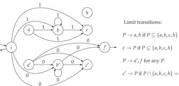
i f a b c h a′ b′ c′ 1 0 1 1 1 1 1 0 0 0 0 0 0 0 Limit transitions: P→a, h if P⊆ {a, b, c, h} c→P if P⊆ {a, b, c, h} P→a′, f for any P c′ → P if P∩ {a, b, c, h} =∅
Figure 4: Automaton checking whether a gap exists in the future
To check whether the formula ϕ is satisfiable by a model which is recognized by an automatonB, we can compute the product of the automatonAϕwithB, and check whether a transition whereAϕoutputs 1 is accessible and co-accessible. This ensures that there exists a successful run of the product automaton going through that transition, meaning that the corresponding input word is accepted by B and there is a position where ϕ holds. This concludes the proof of Corollary 3.
4
Discussion
Logical characterization of automata. We have shown that any LTL, and thus FO, formula can be represented as a non-ambiguous automaton with output. But one can also build such an automaton where the output is the truth word of a property which can’t be expressed as a first-order formula. The automaton shown on Figure 4 outputs 1 whenever “there is a gap somewhere in the future” is true; that formula can’t be expressed in FO. It would be interesting to find a logical characterisation of the properties that can be expressed using such automata.
Computational complexity.The exact complexity of the satisfiability problem for LTL on ar-bitrary orderings remains open. We give a 2EXPSPACEprocedure to compute an automaton
from a formula, whose emptiness can then be checked efficiently. A classical optimization in similar problems is to compute the automaton on the fly, which saves a lot of complexity, so an algorithm using this technique for LTL on arbitrary orderings would be interesting.
Expressive power. On finite and ω-words, LTL restricted to the unary operators (X, F, and their past counterparts) is equivalent to first-order logic restricted to two variables, FO2(<,+1)[8]. Restricting even further to F and its reverse, we get a logic expressively equivalent to FO2(<). In the case of finite words, FO2(<)corresponds to “partially ordered” two-way automata [16]. The proof of equivalence between unary temporal logic and FO2 can be easily extended to the case of arbitrary linear orderings. It would be interesting to find such a correspondence for arbitrary orderings as well, and to see if these restrictions provide lower complexity results.
subformulas that need to be satisfied in particular intervals, and to find a decomposition that shows the satisfiability of the initial formula. Unfortunately it is not clear if and how this can be extended to handle a larger fragment of the logic.
5
Conclusion
We investigate linear temporal order with Until, Since, and the Stavi connectives over gen-eral linear time, and its relationship with automata over linear orderings. We provide a translation from LTL to a class of non-ambiguous automata with output, giving a 2EXPSPACE
procedure to decide satisfiability of a formula in any rational subclass.
This leaves a number of immediate questions, starting with the actual complexity for the satisfiability problem for LTL, but also for some of its fragments, where some operators are excluded. While the full class of automata over linear orderings is not closed under complementation [1], it might still be possible to find a logical characterization for some interesting subclasses.
References
[1] Nicolas Bedon, Alexis B`es, Olivier Carton, and Chloe Rispal. Logic and rational languages of words indexed by linear orderings. In Edward A. Hirsch, Alexander A. Razborov, Alexei L. Semenov, and Anatol Slissenko, editors, CSR, volume 5010 of Lecture Notes in Computer Science, pages 76–85. Springer, 2008.
[2] Alexis B`es and Olivier Carton. A Kleene theorem for languages of words indexed by linear orderings. Int. J. Found. Comput. Sci., 17(3):519–542, 2006.
[3] V´eronique Bruy`ere and Olivier Carton. Automata on linear orderings. In Jiri Sgall, Ales Pultr, and Petr Kolman, editors, MFCS, volume 2136 of Lecture Notes in Computer Science, pages 236– 247. Springer, 2001.
[4] J. Richard B ¨uchi. Transfinite automata recursions and weak second order theory of ordinals. pages 2–23, 1965.
[5] Olivier Carton. Accessibility in automata on scattered linear orderings. In Krzysztof Diks and Wojciech Rytter, editors, MFCS, volume 2420 of Lecture Notes in Computer Science, pages 155–164. Springer, 2002.
[6] Olivier Carton, 2009. Private communication.
[7] St´ephane Demri and Alexander Rabinovich. The complexity of temporal logic with until and since over ordinals. In Nachum Dershowitz and Andrei Voronkov, editors, LPAR, volume 4790 of Lecture Notes in Computer Science, pages 531–545. Springer, 2007.
[8] Kousha Etessami, Moshe Y. Vardi, and Thomas Wilke. First-order logic with two variables and unary temporal logic. Inf. Comput., 179(2):279–295, 2002.
[9] Dov M. Gabbay, Amir Pnueli, Saharon Shelah, and Jonathan Stavi. On the temporal basis of fairness. In POPL, pages 163–173, 1980.
[10] Paul Gastin and Denis Oddoux. Fast LTL to B ¨uchi automata translation. In G´erard Berry, Hubert Comon, and Alain Finkel, editors, CAV, volume 2102 of Lecture Notes in Computer Science, pages 53–65. Springer, 2001.
[11] Hans W. Kamp. Tense Logic and the Theory of Linear Order. PhD thesis, Computer Science De-partment, University of California at Los Angeles, USA, 1968.
[12] Amir Pnueli. The temporal logic of programs. In FOCS, pages 46–57. IEEE, 1977.
[13] Mark Reynolds. The complexity of the temporal logic with ”until” over general linear time. J. Comput. Syst. Sci., 66(2):393–426, 2003.
[14] Chloe Rispal and Olivier Carton. Complementation of rational sets on countable scattered linear orderings. Int. J. Found. Comput. Sci., 16(4):767–786, 2005.
[15] J. G. Rosenstein. Linear Orderings. Academic Press, New York, 1982.
[16] Thomas Schwentick, Denis Th´erien, and Heribert Vollmer. Partially-ordered two-way au-tomata: A new characterization of DA. In DLT ’01: Revised Papers from the 5th International Con-ference on Developments in Language Theory, pages 239–250, London, UK, 2002. Springer-Verlag. [17] A. Prasad Sistla and Edmund M. Clarke. The complexity of propositional linear temporal logics.
J. ACM, 32(3):733–749, 1985.
[18] Larry J. Stockmeyer. The Complexity of Decision Problems in Automata Theory and Logic. PhD thesis, MIT, Cambridge, Massasuchets, USA, 1974.
[19] Moshe Y. Vardi and Pierre Wolper. An automata-theoretic approach to automatic program ver-ification (preliminary report). In LICS, pages 332–344. IEEE Computer Society, 1986.
[20] Pierre Wolper. The tableau method for temporal logic: an overview. In Logique et Analyse, pages 28–119, 1985.
This work is licensed under the Creative Commons Attribution-NonCommercial-No Derivative Works 3.0 License.