HAL Id: hal-01422216
https://hal.inria.fr/hal-01422216
Preprint submitted on 24 Dec 2016
HAL is a multi-disciplinary open access
archive for the deposit and dissemination of
sci-entific research documents, whether they are
pub-lished or not. The documents may come from
teaching and research institutions in France or
abroad, or from public or private research centers.
L’archive ouverte pluridisciplinaire HAL, est
destinée au dépôt et à la diffusion de documents
scientifiques de niveau recherche, publiés ou non,
émanant des établissements d’enseignement et de
recherche français ou étrangers, des laboratoires
publics ou privés.
Formal proofs of two algorithms for strongly connected
components in graphs
Ran Chen, Jean-Jacques Levy
To cite this version:
Ran Chen, Jean-Jacques Levy. Formal proofs of two algorithms for strongly connected components
in graphs. 2016. �hal-01422216�
Formal proofs of two algorithms for strongly
connected components in graphs
Ran Chen1and Jean-Jacques Lévy2
1
Iscas, Beijing & Inria, Saclay 2
Inria, Paris
Abstract. We present formal proofs for the two classical Tarjan-1972 and Kosaraju-1978 algorithms for finding strongly connected components in directed graphs. We describe the two algorithms in a functional pro-gramming style with abstract values for vertices in graphs, with functions between vertices and their successors, and with data types such that lists (for representing immutable stacks) and sets. We use the Why3 system and the Why3-logic to express these proofs and fully check them by computer. The Why3-logic is a simple multi-sorted first-order logic aug-mented by inductively defined predicates. Furthermore it provides useful libraries for lists and sets. The Why3 system allows description of pro-grams in a Why3-ML programming language (a first-order programming language with ML syntax) and provides interfaces to various state-of-the-art automatic provers and to manual interactive proof-checkers (we use mainly Coq). One important point of our article is that our proofs are intuitive and human readable.
1
Introduction
There is a growing interest in programs proofs checked by computer. Proofs about programs are often very long and have to face a huge amount of cases due to the multiplicity of programs variables and the precise details of the programs. This is very frustrating since we would like to explain the proofs of correctness and publish them in scientific articles. However if one considers simple algo-rithms, we would expect to explain their proofs of correctness in the same way as we explain a mathematical proof for a non too complex theorem. This surely can be done on algorithms dealing with simple structures, such as arrays, lists or trees [13]. But we take here the examples of algorithms on graphs where sharing and combinatorial properties holds.
We provide formal proofs for the two classical Tarjan-1972 [17,7] and Kosaraju-1978 [18] algorithms for finding strongly connected components in directed graphs. Tarjan’s algorithm consists in an efficient one-pass depth-first search traversal in graphs which traces the bases of strongly connected components. Kosaraju’s algorithm works with two depth-first searchs on a graph and its reversed com-panion. It uses a post-order traversal allowing to output the strongly connected components one-by-one by considering them in the reversed order of their inter-connectivity. We describe these two algorithms in a functional programming style
with abstract values for vertices in graphs, with functions between vertices and their successors, and with data types such that lists (for representing immutable stacks) and sets.
We use the Why3 system [9,2] and the Why3-logic to express these proofs and fully check them by computer. The Why3-logic is a simple multi-sorted first-order logic augmented by inductively defined predicates. Furthermore it provides useful libraries for lists and sets. The Why3 system allows description of programs in a Why3-ML programming language (a first-order programming language with ML syntax) and provides interfaces to various state-of-the-art automatic provers and manual interactive proof-checkers (we use mainly Coq with a few ssreflect features).
Our proofs are rather short, namely 244 lines for Tarjan (45 lemmas), 312 lines for Kosaraju (34 lemmas) including the program texts. Most of the 89 proof obligations generated by the Why3 system for our Tarjan Why3-ML program are proved automatically, except 5 of them which are manually checked by Coq with a few ssreflect features [6,11]. For Kosaraju, the figures are 59 proof obligations, 2 Coq proofs. There is in fact a balance between automatic proofs and the manual ones in order to keep the readability of these formal proofs.
Our claim is that the details of our formal proofs are human readable and rather intuitive. They will all be explained in our paper. The programs are di-rectly inspired by the ones of the textbooks, but we replaced imperative features by immutable program states. This avoids the cumbersome treatment of memory states and restricts attention to the most important data structures of these al-gorithms. For instance, we do not consider serial numbers for vertices in graphs; we just keep the active parts of the spanning trees, kept in stacks by these two algorithms. But our programs could be refined to the textbooks imperative im-plementations by several steps that we also indicate in this article. We do think that similar techniques can be applied to many other algorithms on graphs.
Finally our article can present a useful step to compare with other formal methods, for instance within Isabelle or Coq [16,12,20,19,10,3,5,4,1,15,14].
The program may look quite inefficient since it deals with lists and sets, but the imperative version is quite efficient as discussed in the conclusion. The next section will present the first algorithm; section 3 presents the pre-/post-conditions and assertions inserted in the program and section 4 will discuss the proof of various lemmas; section 5 shows the possible refinement to imperative programs. In section 6 we present and prove the Kosaraju’s algorithm. We con-clude in section 7.
2
A first algorithm
We consider Tarjan-1972 algorithm [17,7] for finding strongly connected com-ponents in a directed graph. This algorithm consists in a one-pass depth-first search traversal on graphs. It maintains a stack of visited vertices and the rank of the oldest vertex accessible by at most one back-edge in the spanning tree of every vertex. The usual presentation uses the already cited stack and a serial
number for each vertex. In this paper, we adopt a functional programming style and associate to every vertex its rank in the stack of visited vertices.
Our Why3-ML program is based on two mutually recursive functions dfs1 and dfs’ which respectively take as arguments a vertex x and a set of vertices roots and which return the rank m of the oldest vertex accessible by at most one back-edge. Both functions work with a state with three components: the set of black vertices, the working stack and the set of already computed strongly connected components. A set of gray vertices is an extra ghost argument used in the correctness proof, but irrelevant for the algorithm [8]. Thus the state is given by three extra parameters and is returned as the last three components of the quadruple resulting from both functions. Each vertex is white (not visited), gray (under visit), or black (visited). White vertices are defined as non black nor gray.
let rec dfs1 x blacks (ghost grays) stack sccs =
let m = rank x (Cons x stack) in let (m1, b1, s1, sccs1) =
dfs’ (successors x) blacks (add x grays) (Cons x stack) sccs in if m1 ≥ m then
let (s2, s3) = split x s1 in
(max_int(), add x b1, s3, add (elements s2) sccs1)
else
(m1, add x b1, s1, sccs1)
with dfs’ roots blacks (ghost grays) stack sccs =
if is_empty roots then
(max_int(), blacks, stack, sccs)
else
let x = choose roots in let roots’ = remove x roots in let (m1, b1, s1, sccs1) =
if lmem x stack then
(rank x stack, blacks, stack, sccs)
else if mem x blacks then
(max_int(), blacks, stack, sccs)
else
dfs1 x blacks grays stack sccs in let (m2, b2, s2, sccs2) =
dfs’ roots’ b1 grays s1 sccs1 in
(min m1 m2, b2, s2, sccs2)
function rank (x: vertex) (s: list vertex): int =
match s with
| Nil → max_int()
| Cons y s’ → if x = y && not (lmem x s’) then length s’ else rank x s’
end
Graphs are represented by a finite set vertices of vertices and a function suc-cessors which associates to each vertex the finite set of vertices directly accessed
from it by an edge. The working stack is a list of vertices whose head is the top of the stack. The program also uses functions of the Why3 library on sets (add adds an element to a set, mem tests membership to a set, choose picks randomly an element in a set, remove removes an element from a set, and is_empty, union, inter, diff, subset, cardinal all with an intuitive meaning on finite sets) and on lists (Nil, Cons. lmem tests membership to a list, length gives the length of a list, elements returns the set of elements in a list, num_occ gives their number of occurrences). We have two auxiliary functions: rank which provides the order of an element in a reversed list, split which returns the pair of sublists produced by decomposing a list with respect to the first occurrence of an element. Finally max_int() returns +∞ (here the cardinal of the set of all vertices) and min gives the minimum of two integers.
The main program calls dfs’ with the set vertices of all vertices, with empty sets of blacks and grays vertices and an empty set sccs of strongly connected components. Then dfs’ picks randomly a vertex in roots. If that vertex x is white, the function dfs1 is called on it. Then x is pushed into the stack and dfs’ is called on the direct successors of x after turning it to gray. If the returned value is greater than (in fact equal to) the rank of x in the stack, an additional strongly connected component is added to the result by popping from the stack all elements until x. If the returned value is smaller than the rank of x, we return that value after turning x to black. In dfs’, for a non-white vertex, we return the minimum of its rank in the stack and the results from other vertices in the set of roots. If the non-white vertex is already in the set of presently discovered strongly connected components, we return +∞ (namely max_int()).
3
Pre-/Post-conditions
Our graphs are represented by an abstract type vertex, a global constant vertices, and a successors function which gives for any vertex the set of its successors. An axiom specifies that successors of a vertex in vertices stay in vertices. The predicate edge states that two vertices are joinable by an edge.
type vertex
constant vertices: set vertex
function successors vertex : set vertex
axiom successors_vertices:
∀x. mem x vertices → subset (successors x) vertices
predicate edge (x y: vertex) = mem x vertices ∧ mem y (successors x)
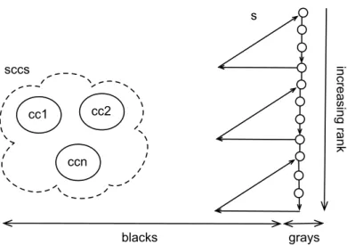
The intuitive proof notices that vertices are stored in the stack in the pre-order of the spanning trees. So for each vertex, the dfs1 function minimizes the rank of vertices accessible from its descendants in the spanning tree by at most one back-edge. When that rank is equal to the rank of its argument, the function dfs1 has met the first vertex of a new strongly connected component the elements of which were pushed in the stack after x. But that proof needs to be formalized. In our paper, we do not introduce spanning trees. We only
cc1 cc2 ccn sccs s grays blacks in cre asi ng ra nk
Fig. 1. Invariants on colors and stack
consider sets of white, gray, blacks vertices. Our formal proof is just based on sets of vertices and the dynamics of the program.
The formal proof relies on two invariants and four post-conditions. The latter ones express the properties of the returned value m in terms of reachability with at most a single back-edge. The former ones are more subtle. They state the relations between colors of the vertices in the working stack and the color of the already computed strongly connected components. Furthermore these invariants show the known reachability between vertices in this stack as illustrated in fig-ure 1. In the Why3-ML language, the first invariant states that the predicate wff_color holds. That means that blacks and grays are disjoint sets of vertices, and that the elements of stack are formed by the union of gray vertices and the blacks which are not in the set sccs of strongly connected components (set_of flattens a set of sets by making the union of all its elements). Furthermore the predicate no_black_to_white says that there is no edge from a black vertex to a white one (i.e. a black vertex can only point to a black or gray vertex). In terms of spanning trees, an equivalent statement is that no node can point directly to a right cousin.
predicate no_black_to_white (blacks grays: set vertex) =
∀x x’. edge x x’ → mem x blacks → mem x’ (union blacks grays)
predicate wff_color (blacks grays: set vertex) (s: list vertex) (sccs: set (set vertex)) =
inter blacks grays = empty ∧
(elements s) == union grays (diff blacks (set_of sccs)) ∧ (subset (set_of sccs) blacks) ∧
The rest of the invariant wff_stack states that gray vertices can reach every vertex with higher rank in the stack and conversely that any vertex in stack can reach a gray vertex with smaller rank. Reachability is defined in terms of paths in the graph by an inductive predicate as in the Why3 library. An additional information simplelist expresses that the stack does not contain repetitions. So the length of the stack is always less or equal to the number of vertices max_int().
inductive path vertex (list vertex) vertex = | Path_empty:
∀x: vertex. path x Nil x | Path_cons:
∀x y z: vertex, l: list vertex.
edge x y → path y l z → path x (Cons x l) z
predicate reachable (x z: vertex) =
∃l. path x l z
predicate wff_stack (blacks grays: set vertex) (s: list vertex) (sccs: set (set vertex)) =
wff_color blacks grays s sccs ∧ simplelist s ∧ subset (elements s) vertices ∧
(∀x y. mem x grays → lmem y s → rank x s ≤ rank y s → reachable x y) ∧
(∀y. lmem y s → ∃x. mem x grays ∧ rank x s ≤ rank y s ∧ reachable y x)
A second invariant characterizes the value of the sccs component in the current state, namely sccs is the set of black strongly connected components. Strongly connected components are naturally defined as maximal sets of vertices connected in both ways by paths.
predicate in_same_scc (x y: vertex) = reachable x y ∧ reachable y x
predicate is_subscc (s: set vertex) =
∀x y. mem x s → mem y s → in_same_scc x y
predicate is_scc (s: set vertex) =
is_subscc s ∧ (∀s’. subset s s’ → is_subscc s’ → s == s’)
The function dfs1 has three pre-conditions expressing that the x parameter is a white vertex in vertices which can be reached from any gray vertex. That function has four post-conditions. The last one says that x is turned to black at end of function. The other three provide properties on the integer m returned by dfs1. Firstly it is less than the rank of x. Secondly it is the rank of a vertex reachable from x. Thirdly if there is an edge from a vertex in the new part of the stack to a vertex y in the old part of the stack, then the returned value m must be less or equal to the rank of that y. These three post-conditions state that the returned value is either the rank of x or of some y in the stack at the beginning of dfs1. We have finally three monotonic post-conditions on the state at end of dfs1. The final stack is a black extension of the initial one, the sets of blacks and strongly connected components are enlarged. The function dfs’ has the same invariants and pre-/post-conditions, upto the set extension to capture the set of roots instead of a single vertex. In fact dfs1 could have been inlined in dfs’, but we feel it is more readable to separate the two functions.
let rec dfs1 x blacks (ghost grays) stack sccs =
requires{mem x vertices}
requires{access_to grays x}
requires{not mem x (union blacks grays)}
(* invariants *)
requires{wff_stack blacks grays stack sccs}
requires{∀cc. mem cc sccs ↔ subset cc blacks ∧ is_scc cc}
returns{(_, b, s, sccs_n) → wff_stack b grays s sccs_n}
returns{(_, b, _, sccs_n) → ∀cc. mem cc sccs_n ↔ subset cc b ∧ is_scc cc}
(* post conditions *)
returns{(m, _, s, _) → m ≤ rank x s}
returns{(m, _, s, _) → m = max_int() ∨ rank_of_reachable m x s}
returns{(m, _, s, _) → ∀y. crossedgeto s y stack → m ≤ rank y stack}
returns{(_, b, _, _) → mem x b}
(* monotony *)
returns{(_, b, s, _) → ∃s’. s = s’ ++ stack ∧ subset (elements s’) b}
returns{(_, b, _, _) → subset blacks b}
returns{(_, _, _, sccs_n) → subset sccs sccs_n}
let m = rank x (Cons x stack) in let (m1, b1, s1, sccs1) =
dfs’ (successors x) blacks (add x grays) (Cons x stack) sccs in assert{inter grays (add x b1) = empty}; (* help provers *)
if m1 ≥ m then begin
let (s2, s3) = split x s1 in assert{s3 = stack};
assert{subset (elements s2) (add x b1)};
assert{is_subscc (elements s2) ∧ mem x (elements s2)};
assert{∀y. in_same_scc y x → mem y (elements s2)};
assert{is_scc (elements s2)};
assert{inter grays (elements s2) = empty}; (* help provers *)
(max_int(), add x b1, s3, add (elements s2) sccs1) end else begin
assert{∃y. mem y grays ∧ rank y s1 < rank x s1 ∧ reachable x y}; (m1, add x b1, s1, sccs1) end
Several features about the Why3 syntax: “requires” and “ensures” are key-words for pre- and post-conditions; “assert” is for assertions in function bodies; “result” is the returned value of a function; “returns” is an abbreviation for “en-sures” with pattern matching when the result is a t-uple.
4
The formal proof
There are a few assertions in the text of dfs1. Most of them are after the split of the stack with respect to the parameter x, which is the critical part of the program since we have to show that we then get a new strongly connected component in the stack on top of x. The first two ones are easily proved. First, the old part of the stack s3 is same as the initial stack, since there are no repetitions in the working stack. The second assertion states that the new part
of the stack s2 (which starts with x ) is all black in the final state of black vertices. The next two are more subtle.
In the third assertion, we prove that the elements of s2 are a subset of a strongly connected component. Indeed take two vertices y and z in s2. Both of them are strongly connected with x since as x is gray in dfs’, we know that x reaches y and z and these two can reach back gray vertices by one invariant at end of dfs’. These gray vertices are with ranks smaller than (or equal to) the rank of x. Therefore they loop back to x.
In the fourth assertion, we prove maximality of s2 as a sub-strongly connected component. So let us consider a vertex y in same strongly connected component as x. We have to show that y belongs to s2. This is a manual proof in Coq that we could not fully automatize. First two automatically proved lemmas implies that if y is not in s2, there is an edge from x’ to y’ both in same strongly component as x such that x’ is in s2 and y’ is not in s2. Furthermore there are three cases. Case 1: y’ in stack. Then either x’ is x, but we know that the result of dfs’ is smaller than the rank of any successors of x, therefore less than the rank of y’ which is then strictly less than the rank of x. Impossible! Either x’ is in the rest of s2, and then there is a cross-edge to y’, contradicting by post-condition of dfs’ that its result is larger than the rank of x. Case 2: y’ in sccs. Then x which is in same strongly connected components as y’ would have to be inside one set of sccs. But the working stack is disjoint from the union of the elements of sccs by invariant wff_color. Case 3: y’ is white. Impossible since x’ in s1 is black and there is no edge from black to white.
The other assertions are proved by automatic provers (Alt-Ergo, E-prover, CVC4, Z3, Spass). The fifth assertion states that s2 is a strongly connected com-ponent. The sixth assertion is a property of boolean algebra on subset ordering that our provers cannot discover. This assertion is used to prove the invariant about colors.
In the other alternative of the conditional statement, there is a single asser-tion. At that point as mentioned above, we know that the corresponding elements of s2 in s1 form a subset of a strongly connected component. But the assertion says that this subset is strict since there is a gray element in it, outside of s2. In fact, we could have called the split function before the test on ranks and made that argument more explicit. But the program would have been further from the textbooks presentation.
The proof obligations in dfs’ are simpler. No assertion is necessary in the body of the function. Only two proofs are to be done in Coq. These are proofs (in two different cases) of the same post-condtion, i.e. m is less than the rank of the ranks of all vertices in roots. There are then many cases because of the min function and the possible +∞ result.
Besides the two functions dfs1 and dfs’, we use lemmas: 5 lemmas about the rank function, 6 lemmas about lists, 17 lemmas about sets(!), 8 lemmas about strongly connected components, 7 lemmas very special to our program.
Detailed proofs can be found athttp:jeanjacqueslevy.net/why3/.
requires{subset roots vertices}
requires{∀x. mem x roots → access_to grays x}
(* invariants *)
requires{wff_stack blacks grays stack sccs}
requires{∀cc. mem cc sccs ↔ subset cc blacks ∧ is_scc cc}
returns{(_, b, s, sccs_n) → wff_stack b grays s sccs_n}
returns{(_, b, _, sccs_n) → ∀cc. mem cc sccs_n ↔ subset cc b ∧ is_scc cc}
(* post conditions *)
returns{(m, _, s, _) → ∀x. mem x roots → m ≤ rank x s}
returns{(m, _, s, _) → m = max_int() ∨ ∃x. mem x roots ∧ rank_of_reachable m x s}
returns{(m, _, s, _) → ∀y. crossedgeto s y stack → m ≤ rank y stack}
returns{(_, b, _, _) → subset roots (union b grays)}
(* monotony *)
returns{(_, b, s, _) → ∃s’. s = s’ ++ stack ∧ subset (elements s’) b}
returns{(_, b, _, _) → subset blacks b}
returns{(_, _, _, sccs_n) → subset sccs sccs_n}
if is_empty roots then
(max_int(), blacks, stack, sccs)
else
let x = choose roots in let roots’ = remove x roots in let (m1, b1, s1, sccs1) =
if lmem x stack then
(rank x stack, blacks, stack, sccs)
else if mem x blacks then
(max_int(), blacks, stack, sccs)
else
dfs1 x blacks grays stack sccs in let (m2, b2, s2, sccs2) =
dfs’ roots’ b1 grays s1 sccs1 in
(min m1 m2, b2, s2, sccs2)
let rec split (x : α) (s: list α) : (list α, list α) =
returns{(s1, s2) → s1 ++ s2 = s}
returns{(s1, _) → lmem x s → is_last_of x s1}
match s with
| Nil → (Nil, Nil)
| Cons y s’ → if x = y then (Cons x Nil, s’) else let (s1’, s2) = split x s’ in
((Cons y s1’), s2)
end
As an appendix, we give the exact definitions of four predicates used in our program assertions, although their names are very explicit. Notice that ++ is the infix operator to append two lists.
predicate rank_of_reachable (m: int) (x: vertex) (s: list vertex) =
predicate access_to (s: set vertex) (y: vertex) =
∀x. mem x s → reachable x y
predicate crossedgeto (s1: list vertex) (y: vertex) (s3: list vertex) = lmem y s3 ∧ ∃s2. (s1 = s2 ++ s3 ∧ ∃x. lmem x s2 ∧ edge x y)
predicate simplelist (s: list α) = ∀x. num_occ x s ≤ 1
predicate is_last_of (x: α) (s: list α) = ∃s’. s = s’ ++ Cons x Nil
We do not consider the main program which calls dfs’ with vertices all white. It remains to show that the black strongly connected components found by our algorithm are the ones accessible from roots. It is the standard proof of depth-first-search that we already proved by itself. Notice too that when the set vertices of all vertices is empty, the empty set is then a strongly connected component, which invalidates our requirement about sccs. So it means that the main program has to check if the set vertices is empty and then returns directly the correct value instead of calling dfs’.
5
Towards imperative programs
It remains to show the proof of the imperative version of this algorithm as ex-posed in algorithms textbooks. We have to suppress membership tests for stack, the calculations about ranks and the operations on sets. The usual technique is to associate serial numbers to vertices in the preorder of the spanning trees, and by giving two exceptional values: −1 for non-visited vertices, +∞ for vertices already in the sets of discovered strongly connected components. Therefore each vertex x has a value num[x], initially set to −1.
We then can refine our program and aim a functional version of the true imperative programs. The state is augmented with the function num and an integer sn providing the next available serial number for the next visited vertex.
let rec dfs1 x blacks (ghost grays) stack sccs sn num =
requires{sn = cardinal (union grays blacks) ∧ subset (union grays blacks) vertices}
(* invariants *)
requires{wff_num sn num stack}
returns{(_, _, _, s, _, sn_n, num_n) → wff_num sn_n num_n s}
(* post conditions *)
returns{(sn_n, m, _, s, _, _, num_n) → sn_n = m = max_int() ∨
∃y. lmem y s ∧ sn_n = num_n[y] ∧ m = rank y s}
let m = rank x (Cons x stack) in
let (n1, m1, b1, s1, sccs1, sn1, num1) =
dfs’ (successors x) blacks (add x grays) (Cons x stack) sccs (sn + 1) num[x ← sn] in if n1 ≥ sn then begin
(max_int(), max_int(), add x b1, s3, add (elements s2) sccs1, sn1, num1) end else
(n1, m1, add x b1, s1, sccs1, sn1, num1)
We return two results m and n respectively the rank and the serial number of the oldest vertex visited with at most one back-edge by the descendants of x. The program flow is identical to the one of the previous functional version since the following invariant relates the ordering on ranks and the ordering on serial numbers.
predicate wff_num (sn: int) (num: map vertex int) (s: list vertex) = (∀x. num[x] < sn ≤ max_int()) ∧
(∀x y. lmem x s → lmem y s → num[x] ≤ num[y] ↔ rank x s ≤ rank y s)
In fact it is convenient to refine the functional program in two steps to the imperative version. First to introduce serial numbers and the num function as we just presented. The second one to modify the split function and modify then the function num as an extra result of split and setting the serial number of popped elements to +∞. We can then test efficiently if a visited vertex is not in the working stack.
6
Another algorithm
Kosaraju’s algorithm is a different way of discovering strongly connected com-ponents in a directed graph. It works with two passes. A first traversal of the graph stores in a stack all vertices in the post-order of their visits. This means that the successors of a vertex are pushed into the stack before that vertex. A second phase iterates on the stack by popping it until a non-visited vertex and performs a depth-first search starting from that vertex on the mirror image of the graph. Then all the vertices encountered by that search form a new strongly connected component. This algorithm may look magic, but its principle is quite simple. It works on the dag of the strongly connected components, and it makes a topological sort on that dag. However it needs to be formalized, and we want here to make a simple publishable proof.
We therefore consider two graphs G1 and G2, each graph is the mirror image of the other one. So the two graphs have the same set of vertices and opposite edges. (We use the module notation of Why3)
axiom reverse_graph: G1.vertices == G2.vertices ∧ (∀x y. G1.edge x y ↔ G2.edge y x)
The function dfs1 performs depth-first search in graph G1, the function dfs2 performs depth-first search in graph G2. Notice that we inlined the recursive calls to the direct successors of a vertex unlike in section 2. The result of dfs1 is a pair the first component of which is the set b of visited vertices. The function works with a state, namely a stack represented by the list stack as argument and returned as s in the second component of the result. We call dfs1 on the
in
cre
asi
ng
ra
nk
s1
gra
ys
st
ack
x
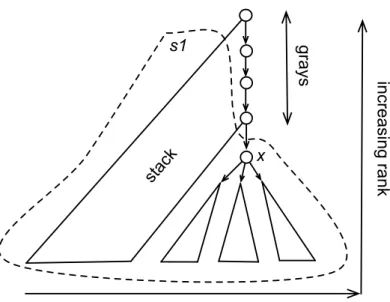
Fig. 2. Invariants on colors and stack in function dfs1
successors of any white vertex x picked randomly in the set roots of vertices after turning x to gray. The function dfs2 performs depth-first search in graph G2. It just returns the set of visited vertices.
let rec dfs1 roots blacks grays stack =
if is_empty roots then (blacks, stack) else let x = choose roots in
let roots’ = remove x roots in let (b1, s1) =
if mem x (union blacks grays) then (blacks, stack) else
let (b2, s2) = dfs1 (G1.successors x) blacks (add x grays) stack in
(add x b2, Cons x s2) in
dfs1 roots’ b1 grays s1
let rec dfs2 roots blacks grays =
if is_empty roots then blacks else let x = choose roots in
let roots’ = remove x roots in let b1 =
if mem x (union blacks grays) then blacks else
add x (dfs2 (G2.successors x) blacks (add x grays)) in
dfs2 roots’ b1 grays
Notice that the vertex x is pushed into the stack at the end of dfs1, namely after the visited vertices from the successors of x (see figure 2). We now dec-orate these two functions with the corresponding pre-/post-condtions and the assertions.
let rec dfs1 roots blacks grays stack =
requires{subset roots G1.vertices}
requires{wff_stack_G1 blacks grays stack}
returns{(b, s) → wff_stack_G1 b grays s}
returns{(b, _) → subset roots (union b grays)}
returns{(_, s) → ∃s’. s = s’ ++ stack ∧
G1.access_from_set roots (elements s’)}
returns{(b, _) → subset blacks b}
if is_empty roots then (blacks, stack) else let x = choose roots in
let roots’ = remove x roots in let (b1, s1) =
if mem x (union blacks grays) then (blacks, stack) else
let (b2, s2) = dfs1 (G1.successors x) blacks (add x grays) stack in assert{not lmem x s2}; (* help provers *)
assert{∃s’. Cons x s2 = s’ ++ stack ∧ G1.access_from x (elements s’)};
assert{no_edge_out_of stack (Cons x s2)};
assert{no_path_out_of_in stack (Cons x s2)}; (add x b2, Cons x s2) in
dfs1 roots’ b1 grays s1
The pre-/post-conditions of that function give the properties of the working stack. This is crucial for the correctness of the overall algorithm. We first require that the set of vertices in the argument roots is contained in the set of all vertices of graph G1 (which are the same as the ones of graph G2 ). The last (monotonic) post-condition states that the set b of visited vertices contains the initial set blacks of already visited vertices given as argument of dfs1. Another (monotonic) post-condition states that the resulting stack s is an extension of the initial stack stack and moreover the extension contains vertices accessible from some vertices in roots. The second post-condition states that this set roots argument of dfs1 is either gray or black at the end of the function. These pre-/post-conditions are just standard properties of any depth-first search on graphs.
predicate wff_color (blacks grays: set vertex) =
inter blacks grays = empty ∧ no_black_to_white blacks grays
predicate wff_stack_G1 (blacks grays: set vertex) (s: list vertex) = G1.wff_color blacks grays ∧ simplelist s ∧ elements s == blacks ∧ subset (elements s) G1.vertices ∧ reachable_before_same_scc s
The important property of dfs1 is that the invariant wff_stack_G1 holds. It states that a property on colors is respected as seen in section 3. Black and gray sets are disjoint and there is no edge in G1 from a black vertex to a white vertex. Moreover the elements of the working stack are vertices in G1. These are again standard properties of depth-first search. But there is an important additional property about reachability within the working stack. Let say that a path starting at a vertex x can reach a vertex y before it within a stack s if each vertex z in that path has a rank in the stack s less or equal to the rank of the final destination y. (The rank function is defined as in section 3). Then the
order in which vertices are stored in the working stack implies that any “path before” has to stay within the same strongly connected component.
predicate reachable_before (x y: vertex) (s: list vertex) =
∃l. G1.path x l y ∧ (∀z. lmem z l → lmem z s ∧ rank z s ≤ rank y s)
predicate reachable_before_same_scc (s: list vertex) =
∀x y. lmem x s → lmem y s → reachable_before x y s → in_same_scc x y
That reachable_before_same_scc property is a fundamental property of span-ning trees with respect to their post-order traversal. The proof of that invariant on the working stack relies on four assertions in the body of dfs1. The first one is just a hint for automatic provers to show the absence of repetitions in the stack. The third assertion states that there could not be an edge from a vertex in stack to another one in s2 not in stack. This is due to the post-order traversal, i.e. no black to white edge in our terminology (see figure 2 where s2 is s1 without x ). So there cannot be a path from a vertex in the old part stack of the working stack to a vertex in its new part s’ with all its intermediate vertices inside s1. This is expressed by our fourth assertion.
Then we can show that reachable_before_same_scc holds in s1. Indeed any “path before” was either already existing in s2 and post-condition of dfs1 called on successors of x was validating the predicate. Either it is a new path in s1, which means involving x. This “path before” needs have x as its last vertex. The fourth assertion implies that that path is totally inside the new part s’ of s1. We know by the second assertion that the elements of s’ are accessible from x. Therefore all elements of the path are in the same strongly connected components.
let rec dfs2 roots blacks grays =
requires{subset roots G2.vertices}
requires{G2.wff_color blacks grays}
ensures{G2.wff_color result grays}
ensures{subset roots (union result grays)}
ensures{G2.access_from_set roots (diff result blacks)}
ensures{subset blacks result}
if is_empty roots then blacks else let x = choose roots in
let roots’ = remove x roots in let b1 =
if mem x (union blacks grays) then blacks else
add x (dfs2 (G2.successors x) blacks (add x grays)) in
dfs2 roots’ b1 grays
The function dfs2 just performs a depth-first search from the vertices in the roots argument and returns the set result of vertices visited by its recursive calls. A post-condition says that the newly visited vertices are accessible from roots. Moreover the following invariant G2.wff_color is verified in a similar way it was holding in function dfs1 for graph G1.
G2.wff_color blacks grays ∧ simplelist s ∧
subset (elements s) G2.vertices ∧ reachable_before_same_scc s
The last function iter2 iterates on the stack computed by dfs1. It pops the stack until its first non black vertex x. Then it makes the singleton set containing x and calls dfs2 with that singleton as roots of the depth-first search. We call cc1 the set of newly visited vertices. Then this set is a new strongly connected component which is stored in the argument sccs which accumulates the set of already discovered strongly connected components. This function iter2 has a few pre-/post-conditions. In fact, the function just requires that the set of white (i.e. non black) vertices are in the argument stack. And it has two invariants, one on the set sccs of strongly connected components (as in section 3). A second invariant wff_stack_G2 is about the structure of the stack. It is similar to the one for dfs1. The only differences are that the stack is not fully black and that the non-black-to-white predicate refers now to G2. Notice that at the end of iter2 the stack is empty and is thus Nil.
let rec iter2 stack blacks sccs =
requires{subset (diff G1.vertices blacks) (elements stack)}
requires{wff_stack_G2 blacks empty stack}
requires{∀cc. mem cc sccs ↔ is_scc cc ∧ subset cc blacks}
returns{(b, _) → wff_stack_G2 b empty Nil}
returns{(b, sccs_n) → ∀cc. mem cc sccs_n ↔ is_scc cc ∧ subset cc b}
match stack with
| Nil → (blacks, sccs) | Cons x s →
if mem x blacks then iter2 s blacks sccs
else
let b1 = dfs2 (add x empty) blacks empty in let cc1 = diff b1 blacks in
assert{subset cc1 (elements stack)};
assert{∀y. mem y cc1 → reachable_before y x stack};
assert{is_subscc cc1 ∧ mem x cc1};
assert{∀y. in_same_scc y x → mem y cc1};
assert{is_scc cc1};
iter2 s b1 (add cc1 sccs)
end
In the body of the iter2 function, we have five assertions with an overall structure similar to the ones of the split case in section 3. The first one says that the set cc1 of visited vertices by dfs2 is contained in the vertices contained in stack. Indeed by post-condition of dfs2, the set cc1 is accessible from the singleton containing x. As x is in stack, it is in vertices by predicate wff_stack_G2. Thus cc1 is a non black subset of vertices, therefore contained in stack by the first pre-condition. The second assertion relies on a lemma which says that any path between any vertices y and z in cc1 can only go through vertices in cc1. This is due to the closing property of reachability induced by depth-first search. Indeed if the path goes through one vertex in sccs, it cannot come back to a vertex in cc1 and similarly if the path cannot go through a white vertex at end of dfs2
since all the reachable vertices from vertices in cc1 have been blackened. In our terminology, this is due to the non-black-to-white predicate before the call to dfs1 and after that call. Now if we take any vertex y in cc1, we know that y is reachable from x by the post condition of dfs2. Therefore there is a path from x to y both in cc1. By the previous lemma, all its intermediate vertices are also in cc1, therefore in stack. This a path of graph G2, therefore a path from y to x in graph G1. But all elements of stack have a rank smaller than the rank of x. So there is a “path before” from y to x, which is the statement of the second assertion.
The third assertion in the body of iter2 is a direct consequence of the in-variant wff_stack_G2 which is true at the beginning of iter2. As there is a “path before” from any vertex y in cc1, we know by the invariant that y is in same strongly connected component as x. Therefore cc1 is a subset of a strongly connected component containing x.
The fourth assertion states the maximality of cc1 as a subset of a strongly connected component. We may use the same lemma as for the second assertion. Let y be in same strongly connected component as x. There are paths from x to y and conversely. So there is a path from x to itself. Since x is inside cc1, all the intermediate vertices on that path are in cc1. Therefore y is in cc1.
The post-conditions of iter2 are shown as in section 3.
We did not consider the main program. It is a call to dfs1 with as arguments the set G1.vertices of all vertices, empty sets of black and gray vertices and an empty stack Nil. The resulting path is then passed as argument of iter2 with empty sets of black vertices and empty set of strongly connected components. The result is the set of strongly connected components of all graph G1 (which are the same as the ones of G2 ). Notice that unlike Tarjan’s algorithm, we could not start with a distinguished set roots of vertices since reachability in G2 is very distinct from reachability in G1.
An appendix of our proof is the following exact definitions of predicates used in our assertions, although their names were very meaningful.
predicate access_from (x: vertex) (s: set vertex) =
∀y. mem y s → reachable x y
predicate access_from_set (roots b: set vertex) =
∀y. mem y b → ∃x. mem x roots ∧ reachable x y
predicate no_edge_out_of (s3 s1: list vertex) =
∀s2. s1 = s2 ++ s3 → ∀x y. lmem x s3 → lmem y s2 → not G1.edge x y
predicate path_in (l: list vertex) (s: list vertex) =
∀x. lmem x l → lmem x s
predicate no_path_out_of_in (s3 s1: list vertex) =
∀x y l s2. s1 = s2 ++ s3 → lmem x s3 → lmem y s2 → G1.path x l y → path_in l s1 → false
Besides the assertions and pre-/post-conditions for functions dfs1, dfs2 and iter2, we use lemmas: 1 lemma about the rank function, 1 lemma about lists, 10 lemmas about sets, 6 lemmas about strongly connected components, 7 new lemmas on paths (reversed graph, path before, path out), 2 lemmas on crossed sets, 3 lemmas very special to our program. In Coq we proved 4 lemmas (3 lemmas about reversed paths and lemma about transitivity of paths), 1 assertion and 1 post-condition (in fact the same assertion about stack extension as in dfs1 for Tarjan’s algorithm).
An imperative version of that algorithm is not difficult to envision although it is slightly technical. Clearly the function dfs1 can be turned into an imperative program by getting mutable maps to describe the colors of any vertex, and the resulting stack can also be constructed in an imperative way. For the second pass, the imperative version is a bit more subtle. We have to give as arguments of dfs2 an existing set sccs of strongly connected components (a set of sets that we may implement as a list of lists) and a connected component cc under construction which would be represented by a list of vertices that we modify when visiting a new vertex in dfs2. Then iter2 stores that list cc into sccs at end of the call of dfs2. Then iter2 goes on calling dfs2. We do not present here the assertions and invariants needed by this imperative version, but it is an interesting development to mimic the textbook algorithm.
Acknowledgments
We thanks the Why3 group at Inria-Saclay/LRI-Orsay for valuable advices.
7
Conclusion
We presented formal correctness proofs of two algorithms in graphs for calculat-ing strongly connected components. These proofs are checked by computer. Most of them are automatically proved. To achieve this, we had to simplify the details of the proofs, which made them publishable in a single article. We think that the details of our proofs are explainable to students who learn algorithms and for-mal methods. This is because of the simplicity of our logic (first-order logic and inductive types), but this is also due to the need for automatization, which de-mands simplification. We however have small bits of these proofs written in Coq and have to check them interactively. Most of the Coq proofs were short, except one in Tarjan’s algorithm. We also took benefits of the functional programming style when presenting these two algorithms. We tried direct proofs of impera-tive versions and had to face more complexity together with lack of readability. It would be interesting to compare our proofs to other formal proofs for these algorithms. Several are existing; they could use spanning trees and therefore be further than our proofs from the real programs and real data structures, but programs might be extracted from these proofs. We also avoided the complexity of separation logic by presenting our functional programs, notwithstanding they are not far from the imperative versions.
Altogether, our approach is quite successful. The proofs are not long, not much sophisticated. We know that there are several flaws with this approach: lack of abstraction, erratic behaviour of automatic provers, uneasy incremental development, no proofs certificates. But we do think that we gained in readabil-ity, which is a very important criterion in formal proofs of programs.
References
1. A. W. Appel. Verified Functional Algorithms. www.cs.princeton.edu/~appel/ vfa/, August 2016.
2. F. Bobot, J.-C. Filliâtre, C. Marché, G. Melquiond, and A. Paskevich. The Why3 platform, version 0.86.1. LRI, CNRS & Univ. Paris-Sud & INRIA Saclay, version 0.86.1 edition, May 2015. http://why3.lri.fr/download/manual-0.86.1.pdf. 3. A. Charguéraud. Program verification through characteristic formulae. In P.
Hu-dak and S. Weirich, editors, Proceeding of the 15th ACM SIGPLAN international conference on Functional programming (ICFP), pages 321–332. ACM, 2010. 4. A. Charguéraud. Higher-order representation predicates in separation logic. In
Pro-ceedings of the 5th ACM SIGPLAN Conference on Certified Programs and Proofs, CPP 2016, pages 3–14, New York, NY, USA, January 2016. ACM.
5. A. Charguéraud and F. Pottier. Machine-checked verification of the correctness and amortized complexity of an efficient union-find implementation, 8 2015. 6. Coq Development Team. The coq 8.5 standard library. Technical report, Inria,
2015. http://coq.inria.fr/distrib/current/stdlib.
7. T. H. Cormen, C. Stein, R. L. Rivest, and C. E. Leiserson. Introduction to Algo-rithms. McGraw-Hill Higher Education, 2nd edition, 2001.
8. J.-C. Filliâtre, L. Gondelman, and A. Paskevich. The spirit of ghost code. Formal Methods in System Design, 2016. To appear.
9. J.-C. Filliâtre and A. Paskevich. Why3 — where programs meet provers. In M. Felleisen and P. Gardner, editors, Proceedings of the 22nd European Symposium on Programming, volume 7792 of Lecture Notes in Computer Science, pages 125– 128. Springer, Mar. 2013.
10. G. Gonthier et al. Finite graphs in mathematical components, 2012. Available at http://ssr.msr-inria.inria.fr/~jenkins/current/Ssreflect. fingraph.html, The full library is available at http://www.msr-inria.fr/ projects/mathematical-components-2/.
11. G. Gonthier, A. Mahboubi, and E. Tassi. A Small Scale Reflection Extension for the Coq system. Rapport de recherche RR-6455, INRIA, 2008.
12. P. Lammich and R. Neumann. A framework for verifying depth-first search algo-rithms. In Proceedings of the 2015 Conference on Certified Programs and Proofs, CPP ’15, pages 137–146, New York, NY, USA, 2015. ACM.
13. J.-J. Lévy. Essays for the Luca Cardelli Fest, chapter Simple proofs of simple programs in Why3. Microsoft Research Cambridge, MSR-TR-2014-104, 2014. 14. F. Mehta and T. Nipkow. Proving pointer programs in higher-order logic. In
CADE, 2003.
15. C. M. Poskitt and D. Plump. Hoare logic for graph programs. In VSTTE, 2010. 16. F. Pottier. Depth-first search and strong connectivity in Coq. In Journées
Fran-cophones des Langages Applicatifs (JFLA 2015), Jan. 2015.
18. M. Sharir. A strong-connectivity algorithm and its applications in data flow anal-ysis. Computers and Mathematics with Applications, 7(7):67–72, 1981.
19. L. Théry. Formally-proven Kosaraju’s algorithm. Inria report, Hal-01095533, 2015. 20. I. Wengener. A simplified correctness proof for a well-known algorithm computing strongly connected components. Information Processing Letters, 83(1):17–19, 2002.