Design and Validation of an Air Window for a
Molten Salt Solar Thermal Receiver
MASSACHUSTS INSTITUTE OF TECHNOLOGYby
JUN
3
0
2010
Adam Taylor Paxson
ES
LIBRARIES
Submitted to the Department of Mechanical Engineering
in partial fulfillment of the requirements for the degree of
ARCHIVES
Bachelor of Science in Mechanical Engineering
at the
MASSACHUSETTS INSTITUTE OF TECHNOLOGY
June 2009
©
Massachusetts Institute of Technology 2009. All rights reserved.
A u th o r ...
...
...
Department of Mechanical Engineering
May 8, 2009
C ertified by ...
...
...
Alexander H. Slocum
Neil and Jane Pappalardo Professor of Mechanical Engineering
Thesis Supervisor
Accepted by...
Lienhard V
Collins Professor of Mechanical Engineering; Chairman,
Undergraduate Thesis Committee
Design and Validation of an Air Window for a Molten Salt
Solar Thermal Receiver
by
Adam Taylor Paxson
Submitted to the Department of Mechanical Engineering on May 8, 2009, in partial fulfillment of the
requirements for the degree of
Bachelor of Science in Mechanical Engineering
Abstract
This thesis contributes to the development of Concentrating Solar Power (CSP) re-ceivers and focuses on the design of an efficient aperture. An air window is proposed for use as the aperture of a CSP molten salt receiver to mitigate efficiency losses due to heat and mass transfer. The current state of the art in CSP technology is outlined with emphasis on molten salt storage. An overview of the theory of air window de-vices is given, and a model is presented which can be used to predict the efficiency of the air window, given by the ratio of prevented heat and mass transfer to aperture power consumption. A design for an experimental test cell is presented, including a method of molten salt simulation and vapor concentration measurement. The test cell demonstrated the ability to lower the mass fraction of vapor outside the aperture by 77.8% ±6.2%. A high rate of cooling was observed in the test cell as the velocity of the air window was increased.
Thesis Supervisor: Alexander H. Slocum
Acknowledgments
In an academic environment where everything and everybody seem to be working at a million miles an hour, I want to express my gratitude to the faculty at MIT who have given their time to assist with my project. My advisor, Alex Slocum, has continually demonstrated that good things come when you have the drive to break the mold and go make a better one. Tom McKrell has proven to be a veritable well of experimental knowledge and know-how; his advice has saved me countless hours of pain and strife. Special thanks to Danny Codd and Stefano Passerini, who have offered consid-erable help and shown a level of calm collectedness uncommonly seen in graduate students. Thanks to my friends who (almost) never gave me a hard time about work-ing too hard on this thesis. Thanks to Ken Stone at the MIT Hobby Shop, who has helped my out of many a fabrication bind.
I want to thank the Cyprus CSP Team for showing me that we scientists and engineers have the power to get something done in trying to fix this world.
Contents
1 Introduction
1.1 Motivation... . . . . . . .
1.2 Concentrating Solar Power . . .
1.3 Molten Salt Storage . . . .
1.4 Air Window Theory . . . .
2 Design of the Test Cell
2.1 Test Cell Overview . . . .
2.2 Concentration Measurement . .
2.3 Air Curtain . . . . 2.4 Chassis Design and Fabrication 3 Experimental Procedure
3.1 Calibration ...
3.2 Concentration Sampling
3.3 Data Acquision . . ...
4 Results and Discussion 4.1 Error Analysis . . . . 4.2 Vapor Pressure . . . . . 4.3 Power Consumption 4.4 Temperature Profiles 4.5 Mass Concentration . . . 43 43 43 44 47 47 48 49 49 51 ... .. .. .. .. .. . . . . . . . . . . . . . . . . . .. . . . . . . . . . . . .. . . . . ... .. . . . . . . . . . . . . ... . . .
4.6 Conclusion... . . . . . . . . 52
List of Figures
1-1 Three variations of solar collectors: dish, trough, and tower . . . . 14
1-2 First-order model of salt losses. . . . . . . . 17
1-3 Plot of estimated salt loss rate vs. wind velocity . . . . 18
1-4 Diagram of receiver concept as proposed by Professor Slocum and his research group... ... 19
1-5 Four zones of an air curtain and corresponding velocity profiles. Uc(x) denotes the velocity along the centerline of the flow, where Ui is the discharge velocity at the centerline... . . . . . . . . . 21
1-6 Power required vs. Flow Quality for commercial air curtains . . . . . 25
2-1 Block diagram of air curtain test cell . . . . 28
2-2 Outer air temperature vs. height along aperture, measured from the bottom edge of the air window . . . . 29
2-3 Molten salt simulation assembly... . . . . . . . . ... 30
2-4 Vapor pressure correlations for salt substitute candidates . . . . 31
2-5 Filtration method of concentration measurement . . . . ... 33
2-6 Concentration measurement subassembly . . . . 36
2-7 Modified outer sampler assembly mounting jig . . . . 37
2-8 Air window assembly. Installed position of pitot tube is indicated by dotted line . . . . 38
2-9 Pitot tube subassembly... . . . . . . . . ... 39
4-1 Measured and predicted (solid curve) mass fraction of n-eicosane vs.
wax temperature... . . . . . . . .. 48
4-2 Air window quality factor 'I vs. power P for varying air window pa-ram eters . . . . 49
4-3 Temperature profiles as a function of air window parameters . . . . . 50
4-4 Vapor concentration difference across air window for varying air win-dow param eters. . . . . 51
4-5 Trails of condensed wax flowing down the inner surface of the enclosure ceiling.. . . . . . . . . 52
A-i Detail section of air curtain test cell . . . . 55
A-2 3rd-angle projection of air window test cell . . . . 56
List of Tables
1.1 Low temperature nitrate salts used in current CSP installations . . . 16
2.1 Characteristics of candidate salt substitute materials . . . . 30
2.2 Results of filtration feasibility test . . . . 35 2.3 Aspect ratios H/e attainable with adjustable air window. Values in
Chapter 1
Introduction
This thesis presents a concept for the aperture of a solar thermal receiver and examines its ability to reduce efficiency losses. The theory of operation of the aperture is explained and applied to the problem of heat and mass transfer losses from a solar thermal receiver. These concepts are applied to the design of a solar thermal receiver aperture test cell. The experimental procedure is described, and the results of these trials are presented along with recommendations for future work.
1.1
Motivation
Global energy consumption is predicted to increase 50 % by 2030, and the anticipated use of fossil fuels to meet this demand is expected to generate to alarmingly high levels of C0 2, NO,, and other environmentally malevolent gases [1, 2]. The current trend in both demand and method of energy conversion is neither environmentally nor economically sustainable. The need for renewable energy technology is becoming increasingly evident, and fortunately large body of work has already been focused on the development of numerous renewable methods of energy conversion. However, there is still need for improvements in efficiency and cost reduction. The large-scale implementation of these technologies, especially for electricity generation, has been hindered by their higher price per kilowatt-hour when compared to conventional fossil fuel sources.
1.2
Concentrating Solar Power
In the pursuit of a cost-competitive renewable source of energy, concentrating solar power (CSP) offers a promising solution. This technology collects solar energy at tem-peratures high enough to supply conventional steam turbines, and can even generate temperature high enough for the thermal production of hydrogen [3]. In addition to being relatively low-cost when compared to photovoltaic and wind technology, CSP has a large resource base and can be installed modularly to further reduce the cost per kilowatt-hour.
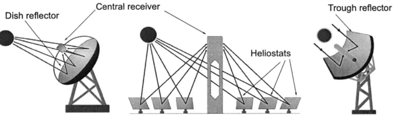
There are several methods of solar thermal concentration, but all rely on the same basic strategy: the sun's energy is focused by an array of mirrors onto a receiver, which then transfers the solar energy to a working fluid. The heated working fluid can then be passed through turbines to generate electricity. The configuration of the collector mirrors, referred to hereafter as heliostats, has a large effect on the efficiency of the plant. The three most commonly utilized configurations are shown below in
Figure 1-1. Depending on the area concentration factor, which is the ratio of collector aperture area to receiver area, the maximum temperature achieved by a typical solar concentrator ranges from 390 C for a parabolic trough collector to 750 C for a dish collector [4, 5].
Central receiver Trough reflector
Dish reflector
Heliostats
Figure 1-1: Three variations of solar collectors: dish, trough, and tower
Although solar troughs are simple to install, their bi-directional focusing and large exposed receiver area present major difficulties to any attempts to increase efficiency. Dish collectors, although offering the highest area concentration factor, are much
more difficult to implement than tower receivers; they require careful measures to achieve a parabolic shape and large actuators to maintain correct orientation with respect to the sun. Of the three most commonly used collector configurations, the solar tower offers the highest operating temperatures for the lowest complexity.
One of the most important factors in determining the efficiency of a CSP plant is the loss of thermal energy from the receiver. In a configuration such as the parabolic trough, a high-temperature receiver tube is exposed to the much cooler surrounding environment over a large area. Both convective and radiative heat transfer contribute to thermal losses in this system. Although measures have been taken to prevent some of these losses, such as the insulation of trough receiver tubes in an outer vacuum shell, unwanted heat transfer from the receiver remains one of the most difficult problems in CSP design. Fortunately, solar towers are able to offset these thermal losses due to their large ratio of collector area to receiver area.
More importantly, solar towers offer the option of energy storage, which is paramount to the commercial success of solar power generation. By storing the thermal energy collected during peak collection hours, the CSP plant becomes much more valuable. The cyclic output of solar plants, which places large stresses on the power trans-mission grid, can be stabilized by the addition of an energy storage element. Power delivery can be controlled to match the periods of increased demand that occur dur-ing non-collectdur-ing hours of the day. Because they focus a large field of heliostats on a single central location, solar towers can offer a more practical scale for storage than trough or dish collectors, which must transfer the thermal energy to a central location with large-capacity storage elements.
1.3
Molten Salt Storage
The most commonly used material for storing thermal energy is molten salt. Current installations, such as Solar 2 in Nevada, have demonstrated that molten salt storage can be commercially viable. Some of the commonly used salts are low-temperature nitrate salts, whose properties are shown in Table 1.1. Although they offer low melting
Table 1.1: Low temperature nitrate salts used in current CSP installations
Property Solar Salt Hitec Hitec XL LiNO3 Therminol VP-1
Composition
[%]
NaNO3 60 7 7 KNO3 40 53 45 NaNO2 40 Ca(N0 3)2 48 Tmeut [0 C] 220 142 120 120 130 Tmax [0 C] 600 535 500 550 400 p [kg/m 3] 1899 1640 1992 1589 P [cp] 3.26 3.16 6.37 0.20 c, [J/kg K] 1495 1560 1477 2319points and minimize the risk of salt freezing in the fluid transfer system, the salts begin to decompose at temperatures seen in solar towers. Because these higher temperatures allow higher cycle efficiencies, it would be beneficial to utilize a salt with higher working temperatures. Some of the salts used by the aluminum smelting industry can withstand much higher temperatures; the neutral chloride mixture Cartecsal has a melting point of 430'C and a maximum working temperature of 950'C.
The storage of high-temperature molten salt has proven to be difficult: high rates of corrosion and high vapor pressures are two of the problems that must be addressed. Depending on the composition of the salt, corrosion effects can be quite severe. Pre-vious work done with nuclear molten salt breeder reactors has resulted in the de-velopment of Hastelloy N, a nickel-based alloy that is able to withstand continuous operation at 704'C with corrosion rates of less than 1mil/yr [61. Unfortunately, this does not solve the problem of designing a high-temperature aperture for a molten salt receiver. A material is needed that has excellent optical clarity. Some attempts have been made to prevent receiver heat losses by covering the aperture with a quartz or sapphire window, only to find that the quartz dissolves upon exposure to the molten salt vapor [7]. Given solar insolation at rates of 50 MW for a typical commercial-sized plant, the required optical quality presents a severe cost limitation.
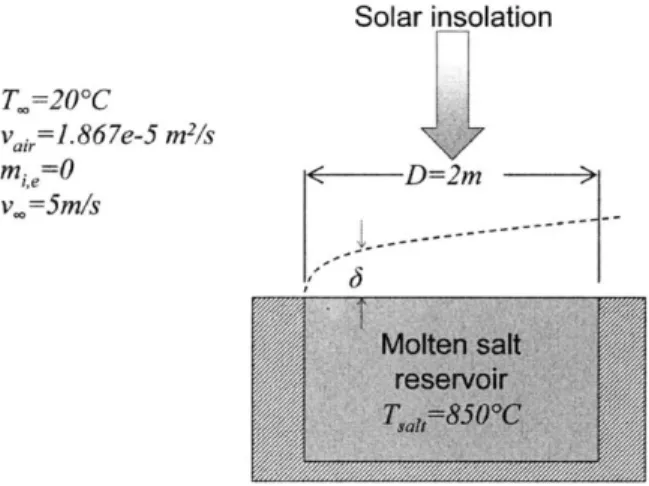
Solar insolation T.=200C Vai =1.867e-5 m2s m.,=: D=2m v.=5m/s Molten saft-reservoir
Figure 1-2: First-order model of salt losses
both thermal energy and expensive salt at a rate determined by salt temperature and composition, and also by the conditions of the receiver and aperture. It is imperative to the design of an aperture that these losses are mitigated. A first-order model of a free surface of salt exposed to convective mass transfer in air is given in Figure 1-2. Dimensions and operating conditions are chosen based on previous work in CSP optics [8] and archived meteorological conditions [9].
The mass fraction of salt just above the free surface at the air-salt interface, m,0
is found by Equation 1.1, where x, is found as Ps,sat/Patm. Ps,sat is found by the Antoine correlation in Equation 1.2, and the values of the constants A, B, and C are provided in the literature [10].
mrO =- XA18 (1.1)
'xzsNols + (1 - Xs,o)Alair
A
log(P) =-- +BlogT+C (1.2) T
The coefficients have been determined experimentally for systems of pure NaCl, KCl, and LiCl. The salt solutions used in the actual plant may differ from these single-species examples, but these values will serve to give an estimate of the vapor pressure behavior of a molten salt system. The loss rate is given in Equation 1.3, which can be assumed for problems of low-rate single-species mass transfer. Values
0.0025 0.005 - ---0.0005 - --- ... --- --- --- --- ---. ----... --- - ---.. .. ..-- - - - -. ---.... ---. 0) 0 2 4 6 8 10 12 14 16 18 20 Wind velocity [n/s]
Figure 1-3: Plot of estimated salt loss rate vs. wind velocity for the diffusion coefficient Dsait,air are taken from the literature [11].
NULPairDsait,air
gm,salt L
NUL = 0.664Re 1/2Sci/2 (1.3)
Dsalt,air
This condition is verified by finding the blowing rate Bm,i given in Equation 1.4. Continuing with the example system of NaCl at 850'C, Bmn,i = 1.27 - 103 << 0.2, so
the condition assumed by Equation 1.3 is valid.
Bmi = mi,s - mi'* < 0.2 (1.4)
1 - mi"s
Given the conditions and dimensions of Figure 1-2, the estimated rate of salt loss is plotted as a function of voo in Figure 1-3. This plot agrees with the value reported in the ASME handbook for NaCl of 0.2 kg/m2/hr. This rate of salt loss from an exposed surface is unacceptable: assuming an average year-round wind speed of 5 m/s, the estimated rate would result in over 20 tons of salt lost per year.
The ideal aperture for a solar thermal receiver should have high optical transmit-tance in the infrared range, low thermal conductivity, and low permeability to molten
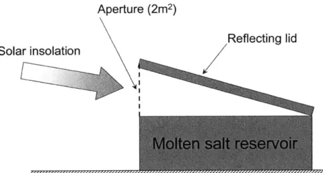
Aperture (2m2)
Reflecting lid Solar insolation
Figure 1-4: Diagram of receiver concept as proposed by Professor Slocum and his research group
salt vapor. This thesis will investigate the two latter specifications of the aperture, and seek to prevent heat and mass transfer from a molten salt receiver. A CSP re-ceiver concept has been proposed by Professor Slocum and his research group that incorporates an air curtain to protect against heat and mass transfer from the molten salt receiver. Slocum's hypothesis is that salt vapor can be constrained to the inside of the lid by the air curtain where it will condense and then be remelted by incoming solar insolation, to then drip back into the container. Figure 1-4 shows a sketch of Prof. Slocum's proposed receiver design (MIT patent pending), in which one of the critical elements is the air curtain covering the opening of the receiver. The capabili-ties of this air curtain need to be characterized so that should it be incorporated into the project, it can be appropriately sized so as to maximize collection efficiency.
1.4
Air Window Theory
Air curtains have been used in both commercial and industrial installations to prevent heat and mass transfer between two areas. Previous studies have demonstrated the
ability of air curtains to inhibit mass transfer of smoke and carbon monoxide [12], particulate diffusion [13], and heat transfer [14]. Proper dimensioning of the air curtain also allows the device to withstand a pressure differential, which can effectively
stop pressure-induced flow within a duct [15]. These capabilities may be applied to the design of a solar thermal aperture, where the principal functional requirements are prevention of heat and mass transfer from the inner receiver zone to the environment. The design of air curtains has proven to be difficult, and many attempts have been made at modeling the behavior of air curtains when they are subjected to pressure, heat, and concentration differences.
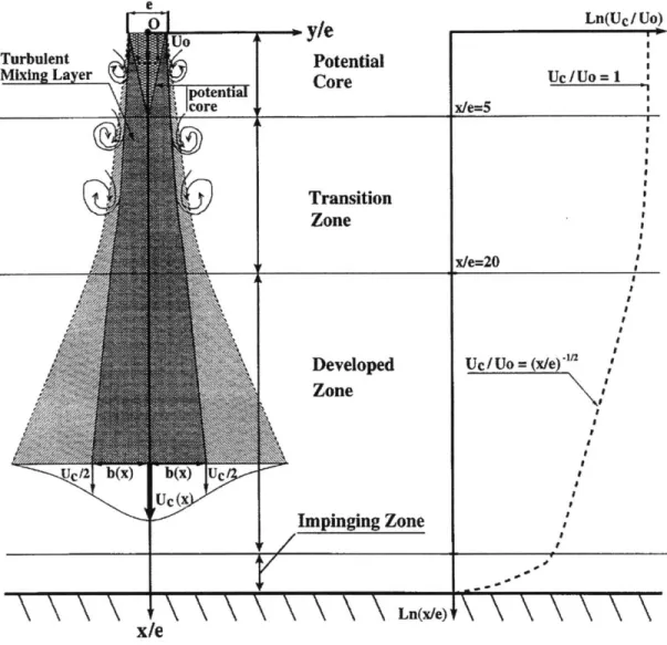
In order to properly size the width and length of the air curtain, it is essential to have an understanding of the velocity profile. The jet from an air curtain can be described analytically by dividing the flow into four different zones: the potential core zone, the transition zone, the developed zone, and the impinging zone [16]. The variation of the velocity profile throughout the four zones can be seen in Figure 1-5 . The dimensionless parameter x/e is used to describe the longitudinal distance of the flow from the inlet. The potential zone can be approximated as the entry region of the air jet; within this zone, the velocity along the centerline of the flow is not affected by the turbulent mixing layer and remains at the initial velocity U,. This correlation will allow for determination of volumetric flow through the air curtain from a measurement of velocity at any point along the centerline, and roughly at the x-location of the opening.
The transition zone begins at a distance approximately 5-8 thicknesses e from the entrance. The velocity profile in this zone is given in Equation 1.5, where or is an empirical constant equal to 13.5 [17]. It is seen from this correlation that the velocity along the centerline begins to decay with increasing x, and assumes a parabolic shape along a constant x-section. It is also important to note that the velocity decreases approximately linearly as jet thickness e. This dimension, and the height of the air curtain H, together form the aspect ratio of the air curtain, H/e. This ratio is a critical aspect of air curtain design. Studies by Guyonnaud and Solliec have verified experimentally the correlations of Equation 1.5 for aspect ratios 10 < H/e < 40.
U(x, y) _1
[~
y
e/2~
15U0 - 1 + erf l (1.5)
UC/2 Dtx) DMX UC Uc ( - y/e Potential Core Transition Zone Developed Zone Impinging Zone Ln(Uc/ Uo) UC /UO=1 x/e=5 x/e=20 a I Uc/Uo=(x/e) 5 I I *
\ \\\L
e)
x/eFigure 1-5: Four zones of an air curtain and corresponding velocity profiles. Uc(x) denotes the velocity along the centerline of the flow, where Uj is the discharge velocity at the centerline
The velocity profile in the developed zone, which begins at a distance of approxi-mately 20e along the air jet, can be described by Equation 1.6, and the velocity along the centerline x = 0 can be described by Equation 1.7, where constants C1 and C2
have been determined experimentally by Schlichting [17] to be 2.45 and 1, respec-tively. Depending on the geometry and discharge velocity of the air curtain, the flow may enter the impinging zone before it can assume the velocity profile described here, i.e., if the total length of the jet is less than 20e. This last zone has been shown to comprise approximately 15% of the total height of the air curtain [18].
U(,=y) _ =6-1 - tanh2 7.67-)1
(1.6)
UO 2 x _y
Uc(x) 02) -1/2
(1.7)
UO e
Although a large body of work has been devoted to the study of an air curtain in opposition to a pressure gradient, we are more interested in air curtains which are in opposition to temperature and concentration gradients. Bragg and Bednarik [13] give an analytical model of the concentration gradient across an air curtain, given in Equation 1.8, where m = 2SchT and depends on the Schmidt number Sch =v/Di,m,
and where ai 1, ai = ak1(m + k - 2).
oo
0(7) = C12m [ ()k a1)!(m ± 2k - 2)
+ C12m S(-1)k+1 ak (m+2k-2)1ooj (1.8)
.k=1 (k -1)!(m + 2k - 2)
The dimensionless concentration O(T) is represented by Equation 1.9, where ' is equal to -(x/y) and u has been determined experimentally to be 7.67.
( C (X, Y) - Cmin (1.9)
Cmax - Cmin
molten salt system, where SchT=0.795 and m=1.59, to the expression in Equation 1.10.
O(TI) = arctan(SchTr) (1.10)
Bragg and Bednarik investigated an air curtain system which included a collection area at the end of the jet instead of a perpendicular impingement plate, as seen in the studies by Guyonnaud et al. By using the simplified result of Equation 1.8, Bragg and Bednarik were able to determine the total mass of disperse particles blocked by the air jet, given in Equation 1.11, where p is the particle density, V is the average volume of the particles, 'i is the average jet velocity at the end of the jet, A is the cross-sectional area of the end of the jet, and 6 is the average value of 0(,q) in the jet
(~0.5 for the fully-developed case).
W = pVuAO(cmax - Cmin)t (1.11)
The approximate cross sectional area of the end of the jet can be found by setting the right-hand side of Equation 1.6 equal to 1% at x/e = 20 and finding the value of y at the edge of the boundary layer. The velocity at the end of the jet can be found with Equation 1.7 at x/e = 20. Combining these results into Equation 1.11 and dividing by t, we can determine the mass flow rate of vapor that is kept from escaping the chamber, given in Equation 1.12. Note that the mass flow rate can be written as a function of four air curtain parameters: inlet velocity Uc,O, air jet length L, jet thickness 6, and jet width w. Additionally, cmin can be eliminated, as the ambient concentration of salt is negligible. cmax can also be written as a function of temperature (given the Antoine equation coefficients describing the salt vapor pressure as a function of temperature) so that the mass flow rate of salt vapor depends only on the salt properties, the four air curtain parameters, and salt operating temperature.
mvapor
= pV
Uc(C1
-C2
w6-206 2 -0.01 L
2 tanh-1 - 7 e- O(Cmax - Cmin) (1.12)
7.67 v/3 767e
Cmax(T) = Pvap(T) (1.13)
RT [Pvap(T)Msalt + (1 -";T Mair
A model for the heat transfer normal to the air window is also needed for the prediction of the performance of the air curtain aperture. Ge and Tassou present a correlation model that has been experimentally validated [19], and is given by Equation 1.14 where rha is the mass flow rate of the air curtain, h. is the enthalpy of the ambient air, T, is the ambient temperature, AT is the temperature difference between the air curtain inlet and the inside chamber, and Ljet is the length of the air jet.
Ma [-0.18h2 + 303.18h, - 0.78(To + AT)2
]
Liet 0
+ "e [216.309(To + AT) - 0.448ho(To + AT) + 509.975 (1.14)
Ljet
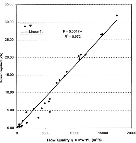
Although the aforementioned models of air curtains offer detailed descriptions of the flow profiles and heat and mass transfer impedance, they cannot be used to accurately represent the power requirements of the air curtain blower. A brief study was conducted of the current state of the art in commercial air curtains to determine the relationship between the power and flow characteristics of air curtains. In order to characterize the flow, a parameter is needed which includes the fundamental elements of the flow. A turbulent jet can be described by four parameters: width w, length
L, jet thickness 6, and velocity v. Since the power requirement of an air jet will be
35.00 30.00 - --- - --- --- --- Linear fit P = 0.001 7W R2 = 0.972 25.00 - --- ---20.00 --- - ---15.00 --- ---10.00 - --- --- --- --- -5.00 --- --- ---0.00 0 5000 10000 15000 20000 Flow Quality T = v*w*t*L (m%/)
Figure 1-6: Power required vs. Flow
Quality
for commercial air curtainswLov to characterize the quality of the flow for different sizes of air curtains. A search
was conducted of several blower manufacturers to gather the power requirements and flow parameters, and the result of power P vs. flow quality T is shown in Figure 1-6.
A linear fit of the data shows that P(T) = 0.0017.
We can now define the efficiency of the air curtain as the ratio of saved power (relative to the case without an air curtain) to the power required by the blowers. The saved power is a function of both entrained salt vapor and the heat transfer across the air curtain. When simplified, we see that efficiency does not depend on the width w, which is expected, given that the heat and mass transfer properties have
Srh
apor(T, V, W,6, L) - cp,vaporT -
Q(T,v,w,6, L)
0.00174'(v, w, 6, L)
The functional requirements of our system necessitate the use of a system that is different from those seen in the work done by Bragg and Bednarik or Guyonnaud and Solliec. In the former case, the purpose of the air curtain system was simply to prevent transfer of aerosol particles across the air curtain, and no concern was given for loss of particulate matter. In the latter case, the purpose of the air curtain system was to oppose a pressure differential in a duct and prevent flow. The proposed air curtain system must be able to prevent both heat and mass transfer normal to a vertical plane at the opening of the aperture. The preceding model for air curtain efficiency might not apply to the conditions experienced by the proposed air curtain on the CSP molten salt receiver, and so must be validated experimentally.
Chapter 2
Design of the Test Cell
To gain a better understanding of the capabilities of an air curtain system for use in a solar thermal aperture, a test cell was developed to simulate the operating en-vironment of a CSP installation. The principal design challenge was to create an accurate representation of the operating conditions using the simplest methods avail-able. Measurements of interest included the temperature profile of the receiver, the vapor concentration on both sides of the air curtain, the flow characteristics of the air curtain, and the power consumption of the air curtain blowers. From these mea-surements, it was possible to determine the efficiency of the air curtain. Due to the time constraints of this study, careful consideration was given to the construction and measurement methods used by the test cell. Although a more elaborate apparatus would undoubtedly yield more accurate results, the final test cell was nevertheless able to produce valuable information with a reasonably small degree of complexity.
2.1
Test Cell Overview
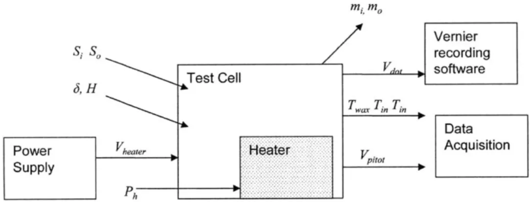
A block diagram of the test cell is shown in Figure 2-1. The variables input to the system are heater power Ph, blower voltage V, air window thickness 6, air window length L, outer sampler toggle So, inner sampler toggle Si, and exposure time t. The measured output variables are wax temperature T., inner chamber temperature
mi. M0
Figure 2-1: Block diagram of air curtain test cell
blower amperage A, inner filter mass mi, and outer filter mass m.
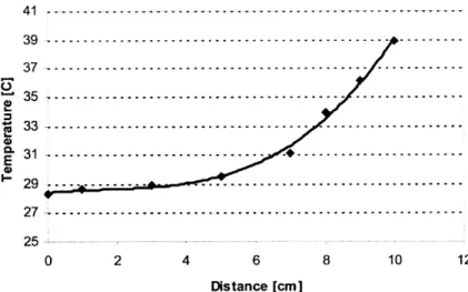
Temperature measurement for the three locations was straightforward. K-type thermocouples were positioned as follows: the thermocouple that measured wax tem-perature was placed so that the exposed end was completely immersed in the wax, but not touching the stainless steel reservoir. The thermocouple that measured the inside air temperature was placed two inches above the center of the wax free surface. The thermocouple that measured the outside air temperature was placed one inch below the top surface of the air curtain blower, and aligned with the centerline of the outer sampling assembly. This location was chosen to gain the most meaningful data from the aperture; the temperature along the height varied considerably due to the convection from the inner chamber. Figure 2-2 shows a typical variation in temper-ature measured along the aperture height, where the distance is measured from the bottom of the aperture opening.
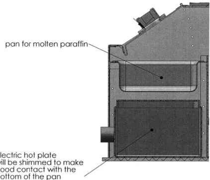
The principal functional requirement of the test cell was dictated by the CSP installation being developed by the MIT Cyprus CSP research group. The proposed test cell shown in Figure 1-4 includes a reservoir for molten salt storage. In order to prevent freezing, the reservoir is maintained at temperatures above the melting temperature of the binary chloride salt: NaCl 50mol% KCl, Tm=660'C. This feature is reproduced by the test cell, shown in Figure 2-3, as an electrically heated reservoir containing a substance that can simulate the vapor pressure behavior of the salt, including freezing, at the lower temperatures attainable by standard lab equipment
41 -39 -37 -35 --- --- -33 --- ---33 --- - --- ---31 ---~ 29---27--- --- _---25 0 2 4 6 8 10 12 Distance [cm]
Figure 2-2: Outer air temperature vs. height along aperture, measured from the bottom edge of the air window
and materials.
To replicate the behavior of a NaCl 50mol% KCl system operating at tempera-tures of 700-10000C, it was necessary to choose a substitute material that exhibits similar vapor pressures at much lower temperatures. Replicating the temperatures of the proposed CSP plant would require the design of a high-temperature test cell using corrosion-resistant alloys, and would have proven to be prohibitively complicated and expensive. Therefore, a number of candidate substitute materials were compared, in-cluding water, two typical low-temperature salts, and paraffin wax. It should be noted that only single-species low-temperature salts were able to be considered. Although the melting point of the two low-temperature salts would be lowered by mixing more than one species, there are limited data for the properties of binary and ternary salt
mixtures.
The selection criteria included melting (freezing) temperature, vapor pressure be-havior [10, 201, and cost; these criteria are outlined in Table 2.1. The vapor pressure correlation for the NaCl 50mol% KCl was obtained by fitting a power curve to pressure vs. temperature data that were calculated with FACTSAGE.
The vapor pressures as a function of temperature for the candidate materials are plotted in Figure 2-4. The plot indicates that water would require lowest tempera-ture while attaining the target vapor pressures of NaCl 50mol% KCl at 700-1000'C.
pan for molten paraffin
electric hot plate
will be shimmed to make good contact with the bottom of the pan
Figure 2-3: Molten salt simulation assembly
Table 2.1: Characteristics of candidate salt substitute materials
Material Tmet [-C] Pap [Torr] Cost [USD/g]
NaCi 50wt% KCl 660 Pvap(T) = 1.134- 10- 34T'1.76 0.35
Water 0 exp [- - + 22.24 + 0.013T - 0.34 - 10-4T2 + 0.69 In(T)] negligible
Iodide salts (e.g. SnI4) 145 log(Poap(T)) = -2975 + 7.66 3.56
Nitrate salts (e.g. AgNO3) 212 N/A 0.78
0 05 - -004~~~ *.*._water 0 .0. -4 --- --- -..--.- -. -..-..-. --.- -. .-..--.- -. .-..--.--. .-..--.--..-. -..-. -. w a te r. .--.--. .-..--.- .--.- .. .. . -s-- P_iodide salt 0.03 --- --- - - - --- -. -. .. - P_NaC 0.0020406080 0010 >00 a 0- - - -- -0 200 400 600 800 1000 1200 Temperature (*C)
Figure 2-4: Vapor pressure correlations for salt substitute candidates
It would seem that using water as the salt substitute material would greatly simplify the design of the test cell. However, any attempt at measuring the concentration of water would be greatly affected by the ambient humidity. A humidifier/dehumidifier and monitoring system would be required in the test cell. Additionally, the ability of the substitute material to freeze at room temperature is a valuable property that affects the design of the aperture. It has been proposed that the ceiling of the re-ceiver enclosure be cooled so that the vapor may condense and drip back down to the reservoir. Water will not freeze at room temperature, in contrast to the other candidate materials, and would not facilitate the modeling of condensation/freezing phenomena. Due to these limitations, it was decided that water would not be used as a substitute material. The two salt candidates were eliminated due to their high temperature requirements. The vapor pressure correlations of Table 2.1 indicate that the test cell would have to be heated to 400'C if an iodide salt were used. This tem-perature would have limited the materials that could be used to construct the test cell. Therefore, it is evident that paraffin wax is the best option for a salt substitute material.
Because an accurate representation of the molten wax vapor pressure was critical to the validity of this study, it was necessary to know precisely its vapor pressure correlation. Paraffin wax was available in many different molecular sizes, ranging from a carbon number of 20 to more than 100 [21]. As the molecular weight of the
alkane decreases, the melting point decreases, along with the temperatures necessary to simulate NaCl 50mol% KCl. Unfortunately, paraffin wax was found to be mildly toxic, and the vapors released would have necessitated the use of a fume hood or other similar ventilation. Beeswax, which is a nontoxic mixture of alkanes, was considered as an alternative [22]. However, due to the difficulty of determining the composition of such a mixture of various sized waxes, it was decided that the use of a single species of alkane would compensate for the added complexity of ventilation. Therefore, the salt substitute material was chosen to be the alkane with the smallest molecular weight:
n-eicosane (Alfa Aesar 99% C2oH42).
To simulate the vapor pressure of NaCl 50mol% KCl at the lowest temperature of interest (700'C), the n-eicosane had to be heated to 117'C. Higher equivalent temperatures were possible, but were limited by the n-eicosane as it approached its flash point of 160 C. For safety reasons, the maximum temperature of the wax had to be kept at or below 155'C, which corresponded to an equivalent salt temperature of 785'C. The n-eicosane was placed in a stainless steel container, and was heated with a Humboldt Model H-4950 electric hot plate with a power output of 750W. Temperature was monitored by a K-type thermocouple queried by an Agilent 34980A datalogger. The enclosure was insulated in such a way that heat transfer along the aluminum walls both prevented freezing of wax on the walls and allowed vapor to condense and drip back down into the wax reservoir.
2.2
Concentration Measurement
The concentration of wax vapor had to be measured on both sides of the air curtain to determine the rate of salt loss. Again, the principal factors for the candidate measure-ment methods were cost and complexity. Many different methods were considered, including gas chromatography [23, 24], laser scattering techniques [25, 26, 27, 28], and meteorological techniques [29, 30]. Both gas chromatography and laser scattering techniques involved a large degree of complexity. Gas chromatography measurements were shown to be time-consuming and required expensive evaporation cylinders, and
Sliding gate
mooFan
Inside
Filter
enclosure
Outsideenclosure
Figure 2-5: Filtration method of concentration measurement
were not pursued further for use in the test cell. Although laser diagnostics would have offered real-time monitoring of the vapor concentration, it would have required an elaborate optical system that included expensive optical filters, positioning de-vices, a detector, and a source. Also, the measurements would have been severely affected by the turbulent air curtain and temperature gradients in the test cell.
Due to these limitations, a filtration method of wax vapor concentration mea-surement was pursued. Although this method does not offer real-time results, it is relatively simple and inexpensive. This method, inspired by the cascade filtration method of concentration measurement used by Schneider et al. [31], used a filter to collect salt vapor. By measuring the volumetric flow through the filter and the determining resulting mass change of the filter, it was possible to ascertain the vapor concentration. The details of operation are shown in Figure 2-5.
A simple mass transfer model was used to determine the vapor concentration as a function of collector dimensions and collected volume. It was assumed that the concentration inside the chamber has reached steady-state, and that the filter was
able to collect F% of the vapor particles, where the n-Alkane particles were described by Schneider et. al. to have an equivalent aerodynamic diameter of 1 Pm The collector model was given by Equation 2.1, where F is the collection efficiency listed by the filter manufacturer for particles of 1 pm and larger. It was important that the filter was sized to capture the vast majority of vapor particles while still allowing a high enough flow rate to be supplied by a small fan. It was assumed that the mass change of the filter was due predominantly to the accumulation of wax vapor, and that the vapor remained at a uniform concentration within the enclosure during the duration of the sampling period.
AMf ilter Pvap = e(2.1)
FVt
This equation was modified to indicate mass fraction as a function of mass change, shown by Equation 2.2.
mvap (Amfilter)
V4
[pwax - Pair(T)] Pair (T)2 [Pwax - pair (T)]
A bench-level test confirmed the feasibility of this measurement method: a pyrex beaker was filled with loz (wt) of common paraffin candle wax and covered with a paper filter. The beaker was heated on an electric hot plate to temperatures ranging
from 160.0 - 176.6'C. The temperature was measured by immersing a K-type
thermo-couple in the wax and reading the voltage through a multimeter. This measurement had a resolution of 10C. At a temperature of 120'C, the wax was completely melted,
indicating that it was composed of heavier-chain alkanes than the C20H44 that was
used in the actual test cell. As the temperature of the wax was increased beyond 1450C, vapor visibly began to evaporate. When covered with the paper filter, the walls of the beaker began to cloud, and eventually formed drops which flowed down the walls. The exposure temperatures and durations for 11 filters are shown in Table 2.2. Mass changes were measured on a Sartorious model CP2245 4-digit scale. Tem-peratures during each exposure drifted by a significant amount due to the deficient
Table 2.2: Results of filtration feasibility test Filter Exposure [min] Twax [0 C] Am [g]
1 1 170-190 0.0010 2 2 160-170 0.0007 3 5 160-190 0.0080 4 5 160-180 0.0059 5 5 170-180 0.0032 6 5 160-180 0.0015 7 5 160-170 0.0032 8 5 160-170 0.0041 9 5 160-170 0.0027 10 5 160-160 0.0020 11 10 205-205 0.0098
thermostat of the electric hot plate, and are listed as a temperature range for each exposure. Because the exact composition of the wax in this test was not known, the target exposure temperature could not be predicted. Only during the last exposure was a sufficiently large change in mass seen. It was evident from this test that in order to reduce the necessary exposure time and obtain reliable measurements, the wax must be heated to its highest safe temperature.
The test cell used a fan to draw vapor-laden air through a filter, and past a spirometer that measured the volumetric flow rate. The sampling fan was a Rexus model DF124020BH, 40mm in diameter, and it produced a pressure head of 82.3 pascals at 8000 rpm. The filter was a Pall Fiberfilm No. 7212 with a flow rate of 180 L/min/cm2 and a 99.9% retention rate of particles over 0.3 pm. The filter was mounted in a sliding gate that facilitated the swapping-out of different filters. Weighing of the filters was performed with a Mettler Toledo model XS105 5-digit scale. The spirometer was a Vernier Model SPR-BTA with a flow rate range of ± 10 L/s and a nominal output of 60pV
/
[L/s]. A custom adapter was fabricated and mounted at the outlet port of the fan so that the spirometer could be easily swapped between the two sampling locations. The details of this assembly are shown in Figure 2-6.Figure 2-6: Concentration measurement subassembly
The inner sampling assembly was mounted on the ceiling of the receiver enclosure, directly above the wax reservoir. There was sufficient mixing of the vapor and air in the chamber to ensure that the measurements taken at this location agreed well with predicted values of vapor concentration. However, the original mounting locations for the outer sampling assembly were not adequate to capture a representative concentra-tion of the escaping vapor. The natural convecconcentra-tion occurring inside the wax enclosure resulted in a highly non-uniform flow exiting the enclosure. The vapor-laden flow was restricted to the upper portion of the enclosure window, while the original mounting location of the outer sampling assembly was not exposed to this portion of the exiting flow. A modified mounting jig, shown in Figure 2-7, placed the sampling assembly at a location high enough to be exposed to the vapor-laden flow.
2.3
Air Curtain
The design of the air curtain had to allow for adjustment of the three defining jet parameters: initial velocity v, air curtain thickness 6, and air curtain length L.
Ad-Figure 2-7: Modified outer sampler assembly mounting jig
ditionally, the air curtain had to provide measurements of the flow velocity at some point on the inlet so that the flow profile could be determined with the use of the equations of Section 1.4. The proposed design for the air curtain, where both the nozzle vane and the roof of the curtain can be adjusted, is shown in Figure 2-8.
The enclosure ceiling is composed of hinged segments that can be set to one of five different heights. The nozzle thickness is maintained by one of three spacers. The possible H/e ratios range from 49.29 with the thinnest nozzle and longest jet, to a value of 2.88 with the thickest nozzle and shortest jet. Table 2.3 gives the possible aspect ratios.
A variety of velocity measurement methods were considered for the test cell, in-cluding hot wire anemometers, vane anemometers, and fan anemometers. It was decided that the velocity of the air nozzle would be monitored by a pitot tube due to its simplicity and small size; it could be made small enough to fit in the thinnest possible air window (0.063") achieved by the moveable nozzle vane. By measuring the pressure at the center of the air window inlet nozzle, the velocity Uc, was
de--variable height air stream pitot dynamic port
variable width air nozzle
inlet fans: 119 cfm each
-1I inlet
Figure 2-8: Air window assembly. Installed position of pitot tube is indicated by dotted line
Table 2.3: Aspect ratios H/e attainable with adjustable air window.
H and row e are in inches
Values in column H e 0.07 0.16 0.26 0.75 10.71 4.69 2.88 1.43 20.43 8.94 5.50 2.10 30.00 13.13 8.08 2.78 39.71 17.38 10.69 3.45 49.29 21.56 13.27
termined by applying Bernoulli's equation along a streamline. Equation 2.3 shows the simplification for our particular case, where the beginning of the streamline is far from the inlet and the velocity is zero.
(2.3)
2AP(Vitot)
Uc,o = 2P(T)
Pair (T )
The pitot tube instrument consisted of an Omega model PX139 temperature-compensated differential pressure transducer with an output of 0.25 - 4.25V over a pressure range of ±0.3 psi. The differential pressure could be found as AP(Vitot) [Pa] = 1034.214- AVitot. The dynamic pressure port was placed at the end of the air curtain
Figure 2-9: Pitot tube subassembly
nozzle and oriented counter parallel to the air flow. The static pressure port was fastened to the outside of the test cell and oriented so as to prevent erroneous mea-surements due to eddy currents. The excitation voltage was supplied by a constant 5V rail on a DC power supply. The pitot tube subassembly is shown removed from its mounts in Figure 2-9, with its installed position indicated in Figure 2-8.
The air jet was driven by two Vantec model TD9238H 12V 92mm case fans, capable of producing a flow rate of 119 CFM at 4800rpm. The fans were powered by a BK Precision model 1670A DC regulated power supply.
2.4
Chassis Design and Fabrication
The design of the chassis for the test cell followed a methodology that was directed by both the functional requirements outlined previously, and by design rules that facilitated its fabrication. The functional requirements of the test cell chassis were as follows:
" Position a stainless steel reservoir over an electric hot plate
" Position an air curtain adjacent to the reservoir
* Prevent heat transfer through walls and out of enclosure
e Protect fans and other heat-sensitive parts from high temperatures
Following these requirements, the design methodology was then directed by the following rules:
" Minimize complexity
" Minimize size
" Minimize cost
" Maximize modularity
The test cell chassis was designed for rapid manufacture and modular installation of the assemblies described previously. A construction approach that used bent sheet metal was pursued because of its low cost and simplicity. A parametric solid model was created in Solidworks whose driving parameters were the dimensions of the critical parts that would later be installed (i.e., hot plate dimensions, fan dimensions, steel reservoir dimensions). This model allowed the parts to be sized with a minimum of wasted material while ensuring that other parts and assemblies would fit without interference.
Aluminum was chosen as a construction material because of its high degree of machinability and high thermal conductivity. This approach allowed the chassis to meet the functional requirement of offering selective heat transfer: where heat transfer was desired between two or more parts, they were joined in a manner that minimized the thermal contact resistance. In regions of the chassis where heat transfer was undesirable, the parts were joined with an intervening layer of thermally insulating material. To be sure that the plastic case fans were not exposed to damaging temper-atures, that region of the model was reduced to a 1-D heat transfer model shown in Figure 2-10. In the worst case scenario, the adjacent wall is heated to the maximum commanded temperature of the hot plate (215'C), and the fan speed is 0 m/s. It was assumed that the plastic had a melting temperature of 120'C, which is a conservative
Insulation
H H T
T,=210*CT=210 C
//
T.T=2210 0
Rai R Rwai Ri,I Rbracker R2,
Rtt= I R
Figure 2-10: 1-D heat transfer model to verify thermal protection of the Vantec fan value for structural acrylic polymers. For this case, in which only natural convection
would act to cool the fan, Rtot = 14.3 K/W, QH = 6.3W, and QL = 34W. Since
the convective cooling rate is higher than the worst-case heating rate, the thermal insulation between the fan and the hot wall will protect the plastic from melting.
The bent sheet metal parts were designed with the intention of being cut with an abrasive waterjet. This cutting process allowed for very accurate, rapid processing of material, and also allowed for the creation of internal features on two-dimensional profiles. Also, the waterjetting process lent itself to such construction methods as sheet metal forming, where tight tolerances and complex cuts needed to be made over a large area of material. Blind rivets were chosen as the joining method because they required no processing beyond the initial waterjet cuts (i.e., boring or tapping holes). Additionally, they allowed for joints with minimal thermal contact resistance when the aluminum rivet body is pressed tightly against the joined parts. Although blind rivets typically do not require tight tolerances, the through-holes of the blind rivets were dimensioned with consideration to the slightly drafted sides produced by
abrasive waterjets. The OMAX waterjet operated by the MIT Hobby Shop was used to cut the profiles from 0.0625" thick sheets of 6061 aluminum.
The insulation between aluminum parts, and also between the fan-chassis joint, was implemented by 0.031" thick sheets of rubber-bound aramid fibers with a thermal conductivity of 0.16 W/mK and a maximum operating temperature of 2000 C. The outer surface of the chassis was insulated by 0.5" thick melamine foam with a foil jacket, having an effective thermal conductivity of 0.037 W/mK and a maximum operating temperature of 180'C. All joints between moving surfaces, which occurred at the adjustable air window vane and chamber ceiling, were sealed with a flexible silicone rubber gasket with a thermal conductivity of 0.22 W/mK and a maximum operating temperature of 230'C.
Chapter 3
Experimental Procedure
3.1
Calibration
Before the vapor concentration tests could be performed, the test cell had to be calibrated to ensure that an adequate amount of vapor was being collected. 72g of
n-eicosane was loaded into the steel reservoir, and the temperature was commanded
to 200 C. Once the temperature of the wax reached a steady value, filters were loaded into the inner air sampler and exposed to the vapor for varying durations. The mass change of the filters was then obtained from a 4-digit scale. As the sampling time was tripled from 6 minutes to 18 minutes, the mass change underwent a similar scaling of 0.7mg to 0.22mg. Similar results were obtained when the outer air sampler was queried. Further trials led to the adoption of a slightly shorter sampling time of 15 minutes, which still allowed for a sufficiently large mass change of the filter to obtain valid concentration measurements.
3.2
Concentration Sampling
The test procedure for determining concentration vs. air curtain parameters was carried out as follows: the wax reservoir was loaded with 100g n-eicosane and was heated to its steady-state operating temperature. For the purposes of this experiment, steady-state temperature is defined as a deviation of no more than 10C for 5 minutes.
The inside and outside filters were exposed for 15 minutes while the air window was not running; this step served as the control case. After obtaining the control samples, the fan power supply was set to three different voltages: 3.5V, 5.OV, and 7.OV. These values were determined by operating the fans throughout their entire voltage range. It was noted that at supply voltages greater than approximately 7.OV, the convection introduced by the air window was large enough to cool the wax considerably. This in turn led to decreased vapor pressures and insufficient mass change of the filters. Due to the nature of the fans used in the air window, a supply voltage lower than 3.5V was not sufficient to turn the fans. After changing the supply voltage, new filters were exposed for 15 minutes, but only after the system had reached a steady state. Once samples had been taken at different power levels and a particular aspect ratio of H/e, the air window was reconfigured to a different aspect ratio and the above procedure was repeated. Again, each time the configuration was changed, the test cell was allowed to run down to steady state before taking the control reading at a
supply voltage of OV.
For all tests, the hot plate operating temperature was set to 215'C. This had been shown in previous trials to correspond to a wax temperature of approximately 150'C, where this temperature tended to fluctuate by up to ±2'C. Filters were handled with tweezers so as to avoid contamination, and were stored in petri dishes when not being exposed.
3.3
Data Acquision
The three thermocouple voltages, along with the voltage signal from the pressure transducer, were read from a BenchLink 34980A Datalogger interface. The software included with the datalogger generated a real-time plot of the four different channels, and allowed for monitoring of the transient behavior of the test cell. The scan rate of the datalogger was 5 seconds per scan. Volumetric flow from the Vernier spirometer was recorded with LoggerPro software, which could determine the total volume of the flow as the integral of the flow rate. The duration of the exposures was also obtained
from spirometer data, which had a sampling rate of 100 samples per minute and gave clear indications of when the filter gate was opened and closed. Mass measurements on the 5 digit scale were taken as the average of three consecutive measurements. Fan power was read directly from the power supply.
Chapter 4
Results and Discussion
4.1
Error Analysis
Before any of the results can be discussed, it is important to consider the different sources of error introduced into the measurements. The published accuracy of the pressure transducer, 5-digit scale, spirometer, and power supply allow for a straight-forward analysis of the propagation of error for the values in the following figures. However, there were other sources of error that could not be modeled or quantified. First, the measurement of concentration exhibits extreme sensitivity to the mass of the filters. Although utmost care was taken to minimize contamination of the filters, it is possible that dust and other pollutants affected the mass measurements. Addi-tionally, the insertion and removal of the filters from the sampling assembly may have resulted in the removal of filter material. There was also the slow evaporation of wax vapor from the filters due to the vapor pressure of n-eicosane at room temperatures. The flow rates of the sampling fans were at the extreme low end of the abilities of the Vernier spirometer. To account for this possible source of error, the flow rate of the sampling subassemblies was taken as the average flow rate for all sampling runs performed. The resulting value for the sampling flow rate was 0.0373 t 0.0016 L/s. Similarly, the pressure transducer was exposed to a range of pressures that constituted a small portion of its measurement range. Therefore, the transducer voltage was averaged over the entire sampling period at a particular fan power setting.
The resulting 95% confidence values were bars of those values that include velocity temperature measurements taken during confidence value that was too small to be
too small to be incorporated into the error measurements. Similarly, the number of a typical sampling run resulted in a 95% incorporated into the following graphs.
4.2
Vapor Pressure
Figure 4-1 shows both the measured and the theoretical values for n-eicosane con-centration within the enclosure as a function of wax temperature. The difference in values is most likely due to the venting of wax vapor out of the aperture; this phe-nomenon will result in a concentration gradient within the enclosure, and was not included in the mass transfer model. Additionally, the wax will have a temperature gradient that increases with depth. The free surface of the molten wax will be at a lower temperature than the wax immediately next to the thermocouple. Therefore, the vapor pressure right above the surface will be lower than if the entire volume of wax had been at the indicated temperature. This effect was more noticeable at higher temperatures, and led to predicted mass fraction values that were too high.
0.016 0.014 ..-- 8.08...--..-.---0 13.27 0.012 -- 30.00 .. 0.010 -.- 29, ... ... 0.008-- - - - -0.002 --- - - -.---0 -.---0-.---0 -- --- - - --- - - - --- --- -- - - - -0.000 80 90 100 110 120 130 140 150 160 Temperature [C]
Figure 4-1: Measured and predicted (solid curve) mass fraction of n-eicosane vs. wax temperature
![Table 1.1: Low temperature nitrate salts used in current CSP installations Property Solar Salt Hitec Hitec XL LiNO 3 Therminol VP-1 Composition [%] NaNO 3 60 7 7 KNO 3 40 53 45 NaNO 2 40 Ca(N0 3 ) 2 48 Tmeut [ 0 C] 220 14](https://thumb-eu.123doks.com/thumbv2/123doknet/14682096.559483/16.918.154.764.145.397/table-temperature-nitrate-current-installations-property-therminol-composition.webp)
![Figure 1-3: Plot of estimated salt loss rate vs. wind velocity for the diffusion coefficient Dsait,air are taken from the literature [11].](https://thumb-eu.123doks.com/thumbv2/123doknet/14682096.559483/18.918.134.783.92.392/figure-plot-estimated-velocity-diffusion-coefficient-dsait-literature.webp)