A derivation of K. Wilson's equations and applications to current operators in relativistic quantum field theory.

,.,

A DERIVATION OF K. WILSON'S EQUATIONS AND APPLICATIONS TO

CURRENT OPERATORS IN RELATIVISTIC QUANTUM FIELD THEORY

by

Richard A. Brandt

S.B., Massachusetts Institute of Technology,

1963

S

UBMITTED IN PARTIAL FULFILLMENT OF THE

R

EQUIREMENTS FOR THE DEGREE OF

DO

CTOR OF PHILOSOPHY

at the

MASSACHUSETTS INSTITUTE OF TECHNOLOGY

June,

1966

~ .

Signature of Author

• .

(

.

Signature redacted

I

Department of Physics,

13

May

1966

~ .

Certified by

Signature redacted

Thesis Supervisor

Signature redacted

Accepted by ..•.•..••.

,,,,.,;~

.

' - " - ~

-

~ ~ ~

••••••··•···

,

Chairman, Departmental Committee

on Graduate Students

Page 54

MITLibraries

DISCLAIMER NOTICE

Due to the condition of the original material, there are unavoidable

flaws in this reproduction. We have made every effort possible to

provide you with the best copy available.

Thank you.

The following pages were not included in the

original document submitted to the MIT Libraries.

This is the most complete copy available.

2.

A DERIVATION OF K. WILSON'S EQUATIONS AND APPLICATIONS TO

CURRENT OPERATORS IN RELATIVISTIC QUANTUM FIELD THEORY

Richard A. Brandt

Submitted to the Department of Physics on May 13, 1966, in

partial fulfillment of the requirements for the degree of Doctor of Philosophy

ABSTRACT

It is shown that, in any renormalizable quantized field theory, the renormalized field operators satisfy local partial differential field equations. The proof is based on rigorously proved properties of renormalized perturbation theory and is valid

to all orders. The field equations have their usual form except

that products of field operators at the same space-time point are

replaced by current operators proposed by K. Wilson. In neutral pseudoscalar meson theory, Wilson's proposal implies that the

current operator h(x) associated with the product $$ is given by

the limit

lim h(&,x) = lim 1 (x + &)$(x)-E₁(&)*(x)-E2y(&

+F &+o0 E3(0)

for suitable functions E.((E) with singularities at ( = 0. It is

shown that E. exist such that, in each order of perturbation

theory, for 'any product X of field operators,(0|Th(Ex)XI >

converges to(|OTh(x)XIo> in the Schwartz topology on distribu-tions on the spaceJ of C' funcdistribu-tions of fast decrease, and that different such E. correspond to finite renormalizations of the

relevant parameters. These results are applied to present a

finite formulation of quantum electrodynamics. The gauge

invar-iance of this theory is established and is shown to be equivalent to the gauge invariance of the field equations.

Thesis Supervisor: Paul G. Federbush

3.

ACKNOWLEDGMENT

All of the investigations carried out in this thesis were suggested to me by my supervisor, Professor Paul Federbush, to whom

I express my sincerest thanks. Professor Federbush supplied the

essential encouragement, stimulation, and education without which the

thesis could not have been written. He also contributed many of the

ideas and most of the philosophy expressed in the work.

I also wish to thank Dr. Klaus Hepp for a very helpful

private communication.

Finally, I thank Miss Nancy Rogerson for translations and

TABLE OF CONTENTS Chapter I. Chapter II. Chapter III Chapter IV. Chapter V. Introduction

1. Products of Quantum Field Operators at Short

Distances .. ... .. . . . .. .. . .

5

2. Outline . . . . . . . . . . , . . . . . . . . . 18

Wilson's Equations 3. Hypothesis and Equation . . . . . ... . . . . 23

4. Derivation of Regularized Integral Equations . .38 5. Finite Renormalizations . . . . . . . . . . . .54

Derivation of Wilson's Equations

6.

7. Meaning of the Current Equation . . . . . . . .82

8. Derivation of the Current Equation . . . . . . 88

The Current Operator in Quantum Electrodynamics 9. Current Operators and Proper Parts.. . . . . . 100

10. Derivation of Integral Equations . . . . . . .107

11. Examples . . . . . . . . . . . . . . . ... .119

Gauge Invariance 12. Gauge Invariance of the Proper Parts . . . . 126

13. Gauge Invariance of the Field Equations . . . 139

Appendix A. Notations and Conventions . . . . . . . . . . . . . 150

Appendix B. Some Theorems from Functional Analysis . . . . . . 151

Appendix C. The Theory of Distributions . . . . . . . . . . . 153

Appendix D. Bogoliubov-Parasiuk-Hepp Renormalization . . . . .156

References . . . . . . . . . . . . . . . . . . . . . . . . . . 162

Figure Captions . . . . . . .. . . . . .. . . .. . .. . . 165

Figures . . . . . . . . . . . . . . . . . . . . . . . . . . . . 169

5.

Chapter I.

Introduction

1. Products of Quantum Field Operators at Short Distances

The concept of a quantized field operator $(x) was introduced

in 1929 by Dirac, Heisenberg, Jordan and Pauli when they invented

quantum field theory. It has been realized since the classic

inves-tigation of Bohr and

Rosenfeld(l)

in 1933, however, that the symbol

*(x) is physically meaningless since the value of a quantized field

at a given point cannot, in principle, be measured. Bohr and

Rosenfeld showed that physical significance can be attributed only

to averages of field operators over small, but finite, space-time

regions. Thus the fundamental dynamical objects of quantum field

theory are the averages

V'(f)

= k ()(x)

(1.1)

for sufficiently smooth and rapidly decreasing testing functions f(x).

Bohr and Rosenfeld showed that, for quantum electrodynamics,

measure-ments of quantities related to (1.1) will always give a definite

answer and that measuring devices could be constructed capable of

verifying all the predictions of a theory based on such quantities.

It is a remarkable fact that all serious attempts

to

attri-bute a rigorous mathematical meaning to 4(x) have led to essentially

the same conclusion

-

*(x) can only be interpreted as the symbolic

kernel of an operator valued functional f

(f) on a suitable space

of testing functions f(x). This confluence of physical and

mathema-tical intuition, however, while kindling hope for the existence of

quantum field theory, implied that extreme care must be exercised in

handling the fields *(x).

In particular, the product *(x)O(x) of two

quantum field operators at the same space-time point is not immediately defined, no more so than is the product of two distributions. This is a reflection of the physical fact that the interference of the field fluctuations would prohibit a measurement of the individual

field averages and of the mathematical fact that such products cannot

be given a rigorous meaning by averaging with respect to testing functions. This phenomenon can also be understood in terms of Haag's distinction between proper operators, those which operate on the Hilbert space of states, and improper operators (or bilinear forms), those which do not Ma p states into states but which do have finite matrix elements. Thus *(x) is an improper operator whereas *(f) is a proper operator. However, *(x) (x) cannot be interpreted as an

opera-tor at all, not even an improper one.

It was, of course, realized from the start that such products were meaningless. One had only to look at the canonical equal-time

anticommutation relation

(1.2)

or calculate the Green's function (4

iG(,-,)

=-

for some soluble model or in second order perturbation theory to

realize that *(x)V(x) was divergent. It simply had no finite matrix

elements. _{Such products were, however, so extremely essential in}

quantum field theory that they were used anyway. Thvs field equa-tions such as

(ChtreI- jpx, (1.4)

where

(1.5)

7.

were universally considered. Calculations based on such equations

always led to the appearance of numerous divergent integrals, includ-ing those which were supposed to represent the self-energies of the

various particles associated with the fields. Now it was realized by

Dirac and Heisenberg(5) as early as 1934 that (1.5) was not the

appro-priate operator to use in (1.4) but that one should rather consider an expression of the form

j () i

rol1ET )'?'(;K')

The product i(x)*(x') has finite matrix elements with singularities

at x = x' which were supposed to be compensated for by q(x, x'). At

that time, however, both the experimental impetus and the mathematical

toolsfor working with such expressions were lacking. Both of these

deficiencies were removed in the late 1940's with the observations by

Lamb and Rutherford of hydrogen fine structure and by Foley and Ku'ch of the electron intrinsic moment, and with the creation by L. Schwartz

of the theory of distributions. The theoretical physics of that time,

however, was based entirely on the products (1.5). The progress came

in the discovery, by Schwinger, Feynman, Dyson, and others (6), of

covariant methods for isolating the resulting divergences and consider-ing them to represent infinite but unobservable renormalizations of

appropriate masses, charges, and wave-functions. The resulting theory

of QED was, in essence, a well-defined collection of techniques which enabled one to perform the necessary calculations. The need

for renormalization, furthermore, meant that *(x)yl'i(x) was not the

real current in QED and that the field equations for the renormal-ized field operator did not really satisfy equations based on such objects.

8.

A formal solution to this problem was provided by Kkll~n (7

in 1952. He presented a formulation of QED involving only renormal-ized Heisenberg operators in terms of which he expressed the renorm-alization constants. His current operator and consequently his field equations explicitly contained these infinite constants,

how-ever, so that his formalism, although it did provide a convenient method for organizing and performing renormalizations, did not answer the question of whether the renormalized operators satisfied

differ-ential equations involving only finite quantities.

Renormalized relativistic perturbation theory has remained

essentially in this unsatisfactory state until today. A significant

attempt to apply and extend the ideas of Dirac and Heisenberg to provide a more solid mathematical foundation for QED was made by

J. Valatin(8) in 1954. He exhibited the electric current operator

j"(x) in the form (1.6) for the case of a fixed external

electromag-netic field but, for the full dynamical problem, he did not present

an explicit form for j11(x) which was correct beyond the third order

of perturbation theory. Furthermore, even in lowest order he did not

regorously prove the existence of the limit in (1.6). We shall see that this must involve explicit consideration of the distribution theoretic aspects of the formalism.

The ideas of distribution theory were gradually assimilated by physicists in the early 1950's and formed the basis of the "axiomatic"

(9)

formulations of quantum field theory. These formulations were an

9.

not involve specific Lagrangian or field equations. Although they

have proved some general theorems (10), the axiomitists have failed to

achieve a deep understanding of the nature of quantized fields - due

mainly to the lack of any non-trivial examples of such. They have, however, provided a framework in which meaningful questions can be

asked.

During the same period in which the axiomatic program was being

formulated, distribution theory was also being employed in attempts to better understand renormalized perturbation theory. In 1953,

(11)

W. Glttinger showed that, within the Feynman-Dyson diagramatic

framework, the consistent use of distribution analysis could formally

account for some of the divergences and ambiguities in QED. He showed

that the arbitrary division constants, which arise naturally when some of Feynman's algebraic relations are considered from the point of view of distribution theory, replace some of the "divergent" constants which appear in a less careful analysis.

Distribution analysis was applied to perturbation theory at a

more fundamental level by Bogoliubov and Shirkov (12), henceforth

referred to as BS, who unified previous work of Schwinger ,

Feynman , and especially Pauli-Villars on invariant

regulariza-tion. BS did not use field equations but derived the perturbation

expansion for the S-matrix from the principles of invariance,

uni-tarity, causality, and classical correspondence. They showed that

10. then the above principles determine Sn to be given by

S,(,..,

x.)

= in

T(X~xi)

-

X

i

where T is the time-ordering symbol, ( is the Lagrangian (in the

interaction representation) and An is an arbitrary "quasilocal oper-ator":

A (X,-- .)XXI)L)

(x-.)(19

for some polynomial P . To specify the A n's one must specify the chronological pairings

(')x'1(

i

(x-y)

(1.10)

at x = y (in the sense of distribution theory). This arbitrariness can be accounted for either by suitably redefining the T-products or by using the usual values (1.10) and allowing non-zero A 's in

n

(1.8). In either case the arbitrariness is just sufficient to obtain

a finite S-matrix for suitable A 's, so that no divergences occur in

n

this formalism. The construction of field products and field

equa-tions is, however, completely avoided. The price paid is that it requires a very complicated and ad hoc procedure to construct the

An, that the special Pauli-Villars regularizations must be employed,

and that no light is shed on the question of whether the renormalized

fields satisfy differential equations.

Now, although the existence of current operators for field equations is clearly related to the behavior of products of quantum

fields whose arguments approach one another, it is desirable to

under-stand the nature of such products for numerous other reasons. This

behavior should, for example, determine the behavior of scattering amplitudes and Green's functions at large energies or momentum

11. transfers. Also, such products could be used to construct

Hamiltoniar or field operators associated with bound states. It was,

ini fact, in an investigation of these latter operators that further

progress was achieved by Zimmerman(13) in 1958. Zimmerman worked

within the framework of the LSZ formulation of field theory, which, however, as Hepp(14) has recently shown, is implied, in part, by the

Wightman axioms. Zimmermann considered a causal neutral scalar field

A(x) in a theory with one-particle states

im

>

IM

>

eigenstates of P2 with eigenvalues m2 and M2 respectively and which

satisfy

Ko1Aom

* 0

KoIA@)IM>

<o(A(x)A)IM>

(1.11)

He defined the field operator B(x) by

BOO)

=Jim

[Ko1TA()A(-f))M.)O>-' [TA 4,,+)AQY,-)

KO\TAM)A1i01

where

|M,O>

P = 0. He did not prove that the limit (1.12) existed but showed that, if it did exist, it defined a causal scalar field satisfying

the asymptotic conditions. He further showed that the S-matrix for the theory was

S~

4

).

--

L

t

m

M

JJA>)--(~lA()--BsJ

(1.13)

so that B(x) has all the properties of a field operator associated

with the bound state

IM>.

As we shall see in the sequel, the limit (1.12 ) exists in all order of perturbation theory for a renormalizable interaction such

12.

that the limit exists more generally. The unfortunate absence of non-trivial field theoretic models satisfying, say, the Wightman

axioms, however, rendered it impossible to verify such hopes under

realistic circumstances. Thus people(15) were led to consider

sim-pler theories some of whose properties might be possessed by future

realistic theories. Theseexactly-soluble field theoretic models were

brought to bear on the problem of the behavior of field operators

at short distances around 1960 and a number of interesting results

were obtained. Before discussing these, let us review the case of

a free scalar field O(x). This model satisfies the Wightman axioms

but, of course, has unit S-matrix. Here the problem of field

multi-plication has the Wick product as its solution. Thus :$nq.

has finite matrix elements and becomes a proper operator when

aver-aged over a space-time region. Furthermore, the behavior of any

product of fields at short distances is given by Wick's theorem. For example, one has

O(,) y)

-Y) (- y) + '. () ().(1.14)

where (see BS)

apart from terms which + 0 as z + 0. Thus

1(>O4#(y)

i(x-y)

_(1.16)

apart from terms whose matrix elements -+ 0 as x-+ y, so that one can

write

p

).

m

(x) y)

+

i

D

(X

-

X)

(1.17)

13.

compensate those of O(x)o(x - z) as z -+ 0. Now one can form sensible

field equations using (1.17) as the current operator, such as

(D + ( : . (1.18)

(16)

Unfortunately, as Wightman and Epstein have shown, equation

(1.18) has no solutions X(x) which are local fields.

Further progress came in 1959 when Haag and Luzzatto(17)

showed that the renormalized field operators for the point source

Lee model(15) and for the point source neutral scalar meson model satisfied finite field equations. These models are, of course,

non-relativistic but the Lee model possesses a non-trivial S-matrix and

both models possess infinite renormalizations. The equation for the meson field a(k) took the particularly simple form

id(k)

ciaAk)

where

(

1

8))

(

1

0

Next, in 1961, Federbush 8 showed that in his model(15), as

well as in a derivative coupling Boson-Fermion model, the

field operators satisfy local differential equations. Both of these models are relativistic but are two dimensional. The Federbush model,

furthermore, leads to a non-trivial S-matrix. The derivative coupling

(gJl

*)

p7

J'iy)

~~

~

J (K)v y

Jx>)>

(ic9)(Y-~

(1.21)

14.

where

j 1 = i),, T*T(x) Oz- . ' r',y t=f (1.22)

Pree f ieIl value. and to the field equation

Spal~ke.Spac~ikeI 1

(1.23)

Johnson 19) next showed that finite field equations exist for

(15)

the Thirring model ). Here the fermion current was the limit of an appropriately symmetrized non-local product:

-

Ji~j

~

~

~)~/

Lf)

~~6)cV~).4)~A~

g-9

where .1 P = 0 to insure Lorentz invariance. If an external field

$ is present, the terms in (1.24) acquire factors of the form

expU

to insure local gauge invariance. The need for such factors was

Scwige(20). Seril (21)

first indicated by Schwinger Sunmerfield considered a gen-eralization of this model and obtained similar results. All these

models are relativistic but are two-dimensional and lead to trivial S-matrices.

All of the above models differ in essential ways from

relativ-istic non-trivial field theories. Recently, however, K. Wilson(22)

15.

field theory. This suggestion forms the basis of the present work.

Wilson has proposed an hypothesis for the behavior of an arbitrary number of interacting field operators, when evaluated near the same

point. The full hypothesis is stated in 3 and becomes, for the product *$ in neutral pseudoscalar meson theory,

Txe-I)cx)

I

-Et()PWX) +

E/

'%T~)

+

E,(

:Y(Y))

(1.26)

as E -+ 0. Here the E (E) are functions with singularities at ( = 0

and :*$: denotes a generalized Wick product - defined only by the

expansion (1.26) If (1.26) were correct, we could define the

current operator

h()

=)

E )

E,(E

-E(0

)L(>)]

(1.27)

to be used in renormalized field equations such as

rYT

(A)

= 0"

h

) .

(1.28)

In this paper we shall derive this hypothesis from rigorously

proved properties of renormalized perturbation theory and show that equations such as (1.28) are valid to all orders. Our results are precisely stated in the next section but we shll here discuss their

significance. In view of the absence of non-trivial field theoretic

models, a proof of equations like (1.26) - (1.28) to all orders of

perturbation theory is the best that we could hope for at present. The success of QED and derived analyticity properties indicates that something about perturbation theory is correct, and it does incor-porate Lorentz invariance and unitarity. However, the perturbation

16.

expansions break down at small distances - just the domain where the

hypothesis is to be checked. It is unlikely, in fact, that the

ex-pansions converge anywhere. On the brighter side, however, we note

that equations (1.27) and (1.28) and later equations which we shall derive (see equations (9.19) - (9.24), (10.54), (13.4_{0))are very} similar to the exact expressions (1.17), - (1.25) obtained for the

soluble models. Wilson's hypothesis is, in fact, a generalization of the free field Wick products and reduces to Zimmermann's result (1.12) in the case that A is a pseudoscalar field with A coupling. Further-more, we shall show that it is quite capable of handling the gauge

invariance problem in QED. All this leads us to hope that the proposal ia of more general validity than our derivation will indicate.

Let us make a brief philosophical comment concerning, say, the electric current operator (9.22). We see that it explicitly depends

on the electromagnetic field A (x) so that our finite field equations do not exhibit a well defined separation between the Maxwell and

Dirac fields. Thus- concepts such as "bare" mass and charge, defined in the limit of no interaction between the Maxwell and Dirac fields,

have no place in our theory. The interactions can never be neglected. It is when one writes the current simply as *(x)yp*(x), thus

intro-ducing a _{separation between the Dirac and Maxwell fields, that the}

bare parameters make their appearance along with the divergences which serve to indicate the mistake that has been made.

We conclude this section by stating more precisely what we mean by "rigorously proved properties of renormalization theory".

17.

The original renormalization prescription of Dyson(23) and Salam(24) has only been rigorously proved(25) to yield convergent integrals in all orders after the contour of each energy integration has been ro-tated from the real up to the imaginary axis. This can be justified, at best, only when all of the external momenta have an imaginary time-component so that the metric becomes negative definite. Bogoliubov and Shirkov (26), however, have proposed an alternate renormalization prescription which avoids this difficulty by introducing the so-called

"a-representation" for the propagators. The rigorous exposition of this prescription, however, as put forth by Bogoliubov and ParasiJk(27)

is unfortunately rather vague. Their proofs, furthermore, are incom-plete or incorrect in part. K. Hepp , however, has recently

pre-sented a much more precise exposition of the Bogoliubov prescription and has completed and corrected the Bogoliubov-Parasilk proofs. The resulting theory, which we shall call the BPH theory, is summarized

in Appendix D. It is the BPH theory of renormalization which we

18.

2. Outline

The next four chapters can be divided into two sets. In

Chapters II and III we derive Wilson's current equations and in Chapters IV and V we apply them. The actual derivations in II and

III will be for neutral pseudoscalar meson theory, although the

methods can be used to derive similar equations for any renormalizable

field theory. _{Likewise, the applications in IV and V will be to} quantum electrodynamics, although the methods can be used to

inves-tigate or formulate any renormalizable field theory. Chapter II

consists mainly of algebraic arguments. There we perform the necessary counting to establish the formal equivalence of perturbation theories based on field equations with Wilson current equations and the con-ventional (BPH) theories based on Feynman diagrams and subtractions. The actual equations derived from the BPH theory are regularized and Wilson's equations follow only if the interchange of certain

opera-tions is allowed. All calculaopera-tions are performed within the usual

momentum space representations of the equations. In Chapter III we complete the derivation of Wilson's equations by showing that the above interchanges are allowed and that the appropriate limits exist which establish the current equations in position space. Here we employ a number of results from functional analysis and distribution theory. The analysis makes heavy use of the a-representation and its relation

to the momentum representation. _{In Chapter IV we apply the above}

results to present a formulation of QED based on field equations. First we write the general forms for the relevant current operators and define numerous proper part functions. Then we derive integral

19.

equations satisfied by the proper parts and use them to find the explicit forms of the currents. In Chapter V we show that the above

proper parts, as given by the iterative expansions of the integral equations, satisfy the requirements of gauge invariance. We then show that this is equivalent to the gauge invariance of the field

equations - _{including the gauge invariance of the electric current}

operator.

We now proceed to describe the fine structure of Chapters II

-V. _{In 3 we state Wilson's hypothesis and review his use of it to}

write field equations and to derive a renormalized integral equation

for the fermion proper self-energy part E(p) in meson theory. We similarly derive an integral equation for the proper vertex part A(p,q) and then for a general proper part t. All these equations involve three functions R1, 1R, R3 to be chosen so that the integrals

converge. In 4 _{we show that a set of integral equations identical}

to those derived in 3, but involving only regularized functions EM(p), etc., are valid to all orders in perturbation theory

renormal-ized according to the BPH prescription, normalrenormal-ized so that

E(O) = DE(o) = A(0,0) = 0. _{We obtain explicit expressions for the}

R . We show in 6 _{that the regularization can be removed, thus}

es-tablishing the existence of the R , the consistency of the iterative solutions of the integral equations, and the equality of the defined functions with the conventional functions associated with sums of Feynman diagrams.

In 5 we first note the equivalence between a BPH theory with

parameters l = rn, 2 3 = Z normalized so that

) =3

para-20.

meters and normalization and with a specified set of R 's. We then

determine which transformations tw , Ri + {w.', R 'j leave a Wilson

theory invariant. Next we show that changing the normalization points

p, p,q in a BPH theory is equivalent to a finite renormalization of the w. 's and use this to show that a Wilson theory with fixed R 's differs from any BPH theory by finite renormalizations of the w 's. We finally show that the transformations tw , R.j -+ lw.', R.'j

leaving a Wilson theory invariant are exactly those which leave its

current equation invariant.

In

6

RIM(p) = EM(p)GM(p) in terms of the a-representation and relate this

to the integral over k of the function RI(k,p) obtained from RIM(p) by cutting an internal meson line. We then obtain the renormalized

integral equation for RIM(p) with the k-integrand expressed in the

a-representation . We show the limit M -+ can be taken inside the

k-integral, thus completing the derivation of the unregularized

in-tegral equation. In 7 we precisely interpret Wilson's current equation

h~

t-,o

to mean that

r-,-

(h0

x)X

(2.2)

for any product X of field operators, the limit ( + 0 being taken in

the Schwartz topology (see Appendix C) on distributions on the space

of C -functions of fast decrease. For X = i(y) we give an

equi-valent statement to (2.2) in terms of functions V (C,p) defined in

21.

well as numerous results from the BPH theory to give a rigorous derivation of (2.2) for the case X =

*(y)-In 9 we begin our treatment of QED by listing the proper-part normalizations (for H, E, A, and X) implied by our choice of parameters

and by the requirements of gauge invariance. We then write down the

field and current equations. In il0 we define numerous functions

and derive renormalized integral equations for 11, A, X, ii,

r,

E and use them to determine the initially unknown functions occur-ring in the currents. In 11 we illustrate previous concepts by explicitly considering the second order H, the third order A, the fourth order H, and a seventh order A.

In 12 we show that the functions A and E defined by the above

equations, as well as newly defined functions 0r, Qr'

9r

defined by similar equations, satisfy numerous generalized Ward

identities. _{We then use some of these identities to show that 11 and}

X

that the above established gauge invariance of the theory is

equiva-lent to the gauge invariance of the field equations - including the

gauge invariance of the electric current operator jp(x). We then write the electric current equation in a manifestly gauge invariant

Chapter II. Wilson's Equations

3. Hypothesis and Equations

K. Wilson has proposed an hypothesis for the behavior of a product of an arbitrary number of interacting field operators, when

evaluated near the same point. In neutral pseudoscalar meson theory,

the proposal amounts to postulating the existence of an infinite

set of Lorentz-covariant local field operators which commute or

anti-commute with the meson field operator O(x) and the nucleon field

operator *(x) for space-like separations. Wilson calls these new

local fields, which are in one-to-one correspondence with the Wick

products of free fields evaluated at a single point, generalized

Wick products. They are defined only by the fact that they occur

in the expansion of the corresponding ordinary products of field opera-tors evaluated near the same point. A generalized Wick product is

assumed to have the following properties: (a) it has the same

transformation properties under the Lorentz and internal symmetry

groups as does the corresponding ordinary product, (b) its dimension

in mass units is the sum of the dimensions of the factors (here

dim I = 0, dim $(x) = 1, dim $(x) = dim

j(x)

dim X(x) + 1, and (c) it is a (proper) operator-valued distribution

on test functions of space and time.

Specifically, Wilson proposes that any product X(x). X1 ().(X

Xn(Xn) of local field operators has, for the xn all near x (say the

components of x - x are all of order _{,) an expansion of the form}

jal i

j(3.1)

plus terms which -0 (weakly) as the xi -+ x, where: X' 's are more

local operators, each term on the right transforms like the left,

dim X' - dim(X...X _{n),and the E 's (which are matrices in the internal}

variables) are distributions with dimensionsd _{= dim(X- -- Xn) - dim X}

and singularities ) f-dj _{to within a small fractional power oF 1.}

Time-ordered products are supposed to have similar expansions. See

Wilson for more details.

As motivation for the expansion (3.1), Wilson shows that in simple c ases it holds for ordinary Wick products of free fields. Furthermore, the operators appearing on the right are the most general ones which relate renormalized _{field equations (see below)}

to unrenormalized field equations by renormalization. Wilson guessed the behavior of the "singular function" Ej on the basis of perturbation

theory (see below).

We consider now neutral pseudoscalar meson theory. Wilson' s hypothesis states that there exist distributions E and a local

operator :*(x) (y): such that

y-T'((

_{~x~.(xy?~fQ)i-F(-x:y(KP)}

_(3.2)

where :*(x)$(x): , _{the generalized Wick product of i and}

_*,

2

2

-1

'.

hE'

= (X - y), then roughly E 1 #%0

,

equations are solved. _{Stated differently, Wilson proposes that}

2.5.

We

~

~ ~ ~ ~ ~ ~ ~

exists (weakly) and defines :*(x)$(x): . Actually, since (3.3)

involves distributions in &,, the limit is not immediately defined.

We will give a precise definition in 7. We will call equations

of the form (3.3) Wilson equations~for renormalized field operators. Thus, if correct, Wilson's hypothesis tells how to constrict finite

parts of products of local fields, which can be used as current

operators in sensible field equations. For example, Wilson replaces the "unrenormalized" equation

=

9.'5-x)t(x)

_(3.4)

involving the "bare" parameters m and g₀, with the "renormalized"

equation

0,;K- _{'TW If(X)(3.5)}

involving the finite "dressed" parameters m and g. (3.5) is the most general linear equation relating the three spinor fields

(*,* ,0:) of dim < . If the E 's were finite functions, then one sees from (3.3) that the bare and dressed parameters are simply related (by "renormalization"). _{In reality, however, the bare} parameters appear to be meaningless. Wilson calls (3.5) a

renorma-26.

lized field equation and calls a field operator renormalized if it

obeys a renormalized field equation.

Wilson next derives a renormalized integral equation, using his hypothesis to take the usually neglected problems associated with

products of field operators into account in a realistic way. Equal time commutation or anticommutation relations are not assumed. He

defines some vacuum expectation values of time-ordered products of renormalized field operators and their Fourier transforms: (0

i

G(x),;)

=

G(P

(3.6)

D 6,0(3.

₇₎

V(x) i)

K'U)

;P(x-j)

V(r)(38

<M (')'1)

(3.9)

All such vacuum expectation values, to be called "Green's functions",

are assumed to be tempered distributions. It follows from (3.5),

(3.6), (3.8) _{and the assumed spacelike anticommutation of *(x) and *(y)}

that

S

G(Y1(3.10)

for x # y. G must satisfy Feynman boundary conditions with respect

to x₀ (i.e., G(x,y) is a superposition of only positive (negative)

S7.

the most general allowed solution of (3.10) is

G(xd

1)

X-X) ,\/(

-= -,c~dX'G~x-X')Y~-V~',) '(3.11)

where Z is an arbitrary constant (it could be fixed, e.g., by specify-ing some equal-time commutation relation) and

GF(X-Y)

P)

P (3.12)

with

GF

Li)

(3.13)

This assumes the integral in (3.11) makes sense, as it does in perturbation theory.

Wilson next makes the expansion

T 9x)$(}

a

(X-

P) V(X)

+

)

~

) -8(x1:60$x:

( 3.14)

Putting

3(-

)

=

+

133

-

)

(3.15)

(B3 is or order g2 in perturbation theory),oue gets

kx)

(3.16)

28.

as a weak limit. Thus, for x 0 y,

(^)i=

Liw

F(

_,)V(,,

_(3.17)

L-

~

~

Fo~

-,A

t3

G')

6

J.)~"~p

3

Uh)V.(r)J

(3.18)

where _{B (p) are the Fourier transforms of B (x - z). Now Wilson}

assumes the limit in (3.18) can be taken inside the integral. This

is a strong assumption since (3.18) is a distribution in (x - z) whose value at a point need not be defined and since, even if (3.18)

were an ordinary integral, the bracketed term would have to behave

nicely in order to justify the interchange of limit and integral.

Assuming nevertheless that the interchange can be performed, and that

(3.14) also holds at x = y, one gets

\/(P)

F(P)

-O

W

64G

_{(P) -8,(k) P'G W}

_{- 3,W (P<\()j (3.19)}

Actually, Wilson's hypothesis does not specify V(x,y) for x = y.

A 6-function can be added to (3.18)(but not a derivative of a

6-function, by dimensionality), and this would add a term of the

form -B _{4(A) to the integrand in (3.19) and would charge Z by a}

constant in (3.11). The existence of such a 6-function term is clearly related to the question of equal-time commutation relations,

which are not assumed here. _{It turns out that B}

29.

sufficiently ambiguous so that (3.19) will converge without -B ₄(k).

This ambiguity will be discussed in 5. Thus one can define V(x,y)

as the Fourier transform of (3.19), and it will then exist as a

tem-pered distribution.

The Fourier transform of (3.11)is

(3.20)

One defines the "nucleon proper self energy part" E(p) and the "proper vertex part" r(pk) by

G(P)

GFW

+

GF

(3.21)

and

(3.22)

It follows from (3.20) and (3.21) that

(3.23)

Inserting (3.22) and (3.23) into (3.19) gives

Z7(i)

G (p) z -z' Gr: (P)

- i

G,

(P 1,- Vp) .

F

(p I )

=

- G (P+,) PQ,A)G (f)

(4)

-- V\(p)

G

30.

where

(3.25)

(3.26)

(3.27)

We will _{call equations of the form (3.24) renormalized integral} equations. _{The subtractions in (3.16) necessary to define the} current operator :(x)O(x): _{as the finite part of T$(x)o(x) go}

over into subtractions necessary to make the integral in (3.24) finite. R 1and _{R2p correspond to the usual mass and wave-function}

renormali-zation, whereas the subtraction _{-g-1R3E(p) explicitly appears for}

the first time in Wilson's work. Equations similar to (3.21) and (3.24) can be analogously derived for all of the Green's functions

and proper parts in meson theory. These can be solved iteratively and yield perturbation expansions for all quantities of interest. Equation (3.24), for example, tells how to compute Z to any order, provided Gj, D, and Z are known in lower orders. The functions

R₁, R₂, and R3 _{must be chosen so that the integral (3.24) converges,} but otherwise they are arbitrary. This arbitrariness is not

essential and will be discussed in 5. _{Thus, provided all the}

required subtraction functions exist and all the integral equations are consistent with each other, one gets a complete and finite

per-turbation theory. _{That this situation prevails will be shown to follow}

31.

the above iteration procedure of calculation is equivalent to the renormalized perturbation expansion associated with Feynman diagrams.

We now use Wilson's hypothesis to derive an integral equation for

r(pq).

S(x, r ) =: () (

tx)(K ) W()

f9

(p

~Y

f

fJ

E(P,

)

k).

(3.29)

Using (3.5), (3.9), and (3.24) we obtain

(3.30)

for x 0 y, z.

The only solution to (3.30) which is consistent with the Feynman boundary conditions and the dimensionality requirements is

32,

The Fourier transformed equation is

F(P,9)

x 5 G, (pti) 5

(3.32)

It follows from equations (3.21), (3.22), and (3.32) that

-3

D If

(p))

7-(t)G(P(n)

S(+-)G(P+-V)G

G()D

(c)

(3.33)

Now we use (3.16) together with the definitions (3.9), (3.24), and

(3.29) to get

'XJ ri,

L) '

= i ()

V,-V)F(x,

2,.)

u- F

-xi2r) (3'3

)

Introducing the Fourier representation of the quantities in the bracket, and assuming the limit can once again be taken inside the integral, we obtain

(P>

(P,1)

-

Rk

F-

_L3

_{V (P,}

(3.35)

We define a new function Q(p, q, k) by

33,

(3.36)

We also define A(p, k) by

.

(3.37)

Substituting (3.22),

EflGD

+

(3.33), and (3.36) into (3.35) gives (symbolically)

= I _{5JDGArGD -- 183}9_{V-rPGD +}

_GPrGPGD

+II3GPGD

+

G

p G D

DB

(3.38)

+ Y G

D.

Taking (3.24) into account, and using (3.37), we are left with

Ap>)

=

G

(P-)):z

₎

_(3.39)

as our renormalized integral equation for A(p, q).

It is not much more difficult to derive the most general re-normalized integral equation which follows from the rere-normalized field

[(r9, ) =i [(k) G(PA

),

A)G(P -

i)

D

-

G(P-1)

DVct)

8

(0* k)

- iD()G(,-A)

(P) P- f - ) G(o- f) D (f) .

=

_{11 Si,, +}

_A(P>,

_*

34.

define the Green's functions

(3.40)

(3.41)

and

(3.42)

For the remainder of this section we shall write these, and their Fourier transforms, simply as V, E, and F. We omit all position and momentum arguments aince they can easily be supplied by inspection.

The field equation (3.5) implies that

(3.43)

for x 0 y₁,...,w . _{The only solution to (3.43) which is consistent}

with the Feynman _{boundary conditions and the dimensionality} require-ments is (in _{momentum space)}

F

=,GF

_(3.44)

35.

We now define the proper part function 0 by

F (PW2

_(3.45)

where W is the obvious product of G's and D's and the omitted terms involve (assumed) already defined proper part functions

correspond-ing to smaller k and/or X. Using equation (3.21), this becomes

F

=-Z(

G

-

&

G)\V

+

G

)

Comparing (3.44) and (3.46), we see that

The current equation (3.16) implies that

11

[

m E

-8FP. - 13 ~f

(3.46)

(3.47)

(3.48)

Introducing the Fourier representations of the quantities in the

bracket, and assuming the limit can once again be taken inside the integral, we obtain (in momentum space)

(3.49)

if

=JEE-

,F +

3-P

F -&13~1/].

Next we definec the function E by

E

=

₁

Doc

W

/

DGrGCv>W

--where the omitted terms again involve functions corresponding to

3(0.

smaller k and/or

Substituting (3.45), (3.47), and (3.50) into

(3.44) gives

-

w

v

TG

W+

f

G--.

-[)

'

G

E/

+

3

GC\A

-iB;P GPWM + ,39-'1j'(2-dW +Z TW) f---

(3.51)

I'

J[0GrPG4W

+'

14

DGS\

-RG@

Mi

G

vi~w

--

R

(-1W

+IGA/) +-

(3.52)

where we have used

the definitions (3.25), (3.26) and (3.27) of

R ,

R2,

and R

It follows from equation (3.24) that

(3.53)

Taking this into account in (3.52), along with similar relations

between the omitted terms, we are left with

~T

(3.54)

as the general form of the renormalized integral equations (other

than (3.24) and (3.39)) implied by (3.5)and (3.16).

We have not precisely defined the function

E

occurring in

(3.54). It is clear, however, that a combersome algebraic definition,

analogous to equantion (3.36), could be given. It is much easier

to give a definition in terms of Feynman diagrams, after it is

32'.

will be given in 12 in connection with generalized Ward identities,

but there is no need for us to consider it here.

Other types of integral equations, which follow from different current operators and/or different field equations, can similarly be

derived. _{We will consider examples of these in later chapters.}

First we shall take up the derivation of the above results from BPH renormalization theory.

38.

4. Derivation of Regularized Integral Equations from Perturbation Theory

In this section we shall derive from BPH renormalization theory renormalized integral equations-analogous to those derived

from Wilson's hypothesis in the previous section. However, they will have the form

A. .)ROMj (4.1)

where for example DM is a regularized meson propagator, instead of

(3.54). The proof that the right side of (4.1) is the same as the

right side of (3.54) will be given in Chapter III, along with the

more difficult interpretation and proof of the current equation

(3.16). It will follow that the perturbation solution of these

integral equations obtained by iteration gives the same expression

for the renormalized Green's function and proper parts as are

obtained from BPH renormalized perturbation theory. Thus, the

exis-tence of the subtraction functions RH, R2 and R3 and the consistency

of all the integral equations will be established, and the Green's

functions and proper parts will be associated with sums of Feynmanli : diagrams in the usual way.

In W, Wilson considers only equation (3.24). He shows that in

order g2 the functionsR and R2 can be chosen such that (3.24) is

finite.and that in order g , if the conventional lower order G's

r'5 _{and 0's are substituted in the right side of (3.24), then Rl,}

R2, and R3 can be chosen so that the integral converges. We pro-ceed to extend these results to all orders.

39.

The definitions of the functions to be used in this section, by

correspondence with sums of Feynman diagrams, are given in Appendix A.

Note in particular that we take Z = 1. _{We will use the notation F4-*G}

to mean that the function (or, more precisely, net) F is obtained from the Feynman diagram G using the Feynman rules (summarized in Appendix A) and regularized propagators. The corresponding

renorma-lized quantity is denoted by RF.

We first derive a regularized version of (3.24), namely f(A)-G(p+k -M) PPk-, M)R DN. i M) - R,

(k<t4)

- R, (k M) ?,"

-

3

(iM)

R T(P M)]

,(4.2)

In this section we prefix renormalized quantities with an R. Thus RE(p;M) is the renormalized regularized self energy part, whereas

E(p;M) is regularized but unrenormalized. We consider an arbitrary

IPI n'th order (n even) nucleon self energy Feynman diagram

G = G(V_{1,..., Vn,), connecting the vertices}

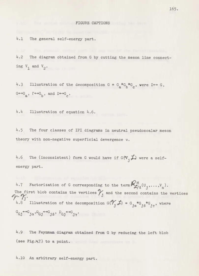
\Y= V1,..., Vn by the lines (, which can be drawn as in Fig. 4.1, where we have

made explicit the O'th order vertices V and V G defines a

corres-ponding regularized self energy part

(4.3)

where gOG1 _{(p, k;M) is the regularized function corresponding to the}

40.

D''(o)

=

D17(Q)

=

1

_{k '}

.

_-

_4.-

_e-(4.4)

Here M symbolically, represents the BP regularization (D4). The

e-dependence of both sides of (4.3) is suppressed since, throughout

this chapter, c > 0 will be fixed.

As is well known, G can be uniquely decomposed into three

parts, G = G *C *G , with

a b

c'

_(")(b

GG7&(Q+j

)"-G

(G

G.

,(?M)

_{= (*Jk'tGa}

_',(

_M)f

_(pk

(k-IM)

(4.5)

This decomposition is pictured in Fig. 4.3. For future reference we note here that any function t(p, ...;M) corresponding to a IPI Feynman diagram with at least one external nucleon line can be

uniquely written in a similar way in terms of a function _E,

corres-ponding to a diagram with an additional external meson line, as follows:

~

12,

Z~ps

~G(+1AM)

~

k

This is pictured in Fig. 4.4. This leads us to define an S-operation on such F's by

Sf(P,---

im)

RG(p4. t, )M) R Z(p, k,.) -

_{M) RD(k,)M).(-7}

Of course, lim S0(p,...;M) will not exist in general.

According to definitions D4 and D5, the renormalized regularized function RE _{G(p;M) corresponding to G is gotten by subtracting from}

(4.5) the sum of the regularized functions corresponding to all

possible contractions of G associated with subgraphs whose superficial

divergences (Def. D3) are > 0. _{Here we have defined a correspondence}

between "contracted" diagrams and terms other than E(n) (p;M)

occur-ring in the sum (see Def. D5).

mv

v

itT

k(P

_~~

_(V~V)

_(4.8)

We call these latter terms "subtractions".

The well-known classes of IPI diagrams with non-negative super-ficial divergences are given in Fig. 4.5. The renormalized function

R G(p) _{corresponding to G is finally obtained by taking limit} (T hm . D4)

to remove the regularization.

RIG(Pr~A = (P M)- SGS (p M) C CGICC,

(4.10)

)-1

We decompose the sum into two parts,

L S-54- (4.13)

the sum being over all contractions in which vertices V and

V2 are not contracted into a generalized vertex, and the sum

being over all contractions in which vertices V and V2 are contracted

into a generalized vertex. Then we can clearly write (4.9) as

Es(i M)

=

-1

_,~S

_"

_(),

_I

_M)

_D'O

_M)

(4.14)

ZTGt(?'IM)

Now we observe that 9 9,(, 1 ')- ) S

(p,

I)

is precisely the regularized renormalized function corresponding _{to G .}

This is because the subtractions one performs in order to renormalize

G never involve contractions of vertex V since vertex V is only

43.

for G corresponds to a unique subtraction for G in which V and V2

are not contracted, namely the one obtained by connecting the meson

lines leaving V₁ and V2 of G. Conversely, any subtraction for G in

which V and V2 are not contracted can be turned into a subtraction

for G_{1 by cutting the meson line connecting V and V This} estab-lishes a bijection between all the subtractions for G and those

subtractions for G which do not correspond to contractions of V and

V2 into a generalized vertex. Our result then follows from the fact,

clear from Def. D6, that if -gS(p,k;M) is a subtraction for G₁, then

-ig S(psk;M)D (k;M) is the corresponding subtraction for G.

'k

Thus we can write

SZ

pV

("('kiM

o 1

(4.15)

where JG is the product

Ga I, G,(4.16)

of regularized renormalized functions corresponding to (4.5). This

is because the way in which a given Feynman diagram is renormalized is independent of any larger diagram in which it is contained.

Thus we will have shown that (4.10) has the form (4.2), with

RGI k -1\/A =

R

r

provided we show that

TG-

(P

)G

(4.19)

for some RG (k;M)'s. This will now be shown to follow from ~Tkm.D2., due to BPH.

By Def. D5, we have

+

X

(4.20)

Let X be the meson line of G connecting V₁ and V₂. Then by equation

(DlO) we have

(j{VI-where is overall IPI

which become IPR without

G,

...

t, and _t

X)

is given by Def. D6 with vertex parts and & --- U -V---

I

)

3(V

)

DP,

T, ( P, ') M )

(V, ... ,)

/

I,

VI---

VO)+14

iA4(V

(vjL.

I...,

,

j

)

.

Consider the first term in (4.21). By Def. D6, the one-particle-irriducibility of a subgraph of G relevant to the construction of an

XX/ is determined only by the lines

/

VI

correspond to V and V2 contracted into a generalized vertex.

However, since

7

subtrac-tion for ,\/) contains A.. Thus we see that in momentum

space

S~iGpM).(4.24)

Next consider the middle terms in (4.21). The vertices

V

which compose a possible V

V

must be such that G(fy,,;() is IPI whereas G('4, '/

)

So clearly V c- and V₂ . Now by Fig. 4.5, the only

genera-lized vertices with non'ynegative superficial divergence and contain-ing an external nucleon line are of the form Z or A. If, however, G( Yj,-- 2) were of the form E, then G would be of the form shown

in Fig. 4.6 and hence could not be IPI (since t<Y(j) Cr').

This would contradict the definition of EG, and so G(

,

be of the form A. _{Thus each term .M VjV}

corresponds to a factoring of G into the form of Fig. 4.7, where G(V, , )4-+ AGJ and G('Y-yj, )++AGj. Here A need not be a

i

Gj

Gj-Gj

proper vertex part.