Mapping water ice clouds on Mars with MRO/MARCI

HAL Id: hal-03104116

https://hal.archives-ouvertes.fr/hal-03104116

Submitted on 8 Jan 2021

HAL is a multi-disciplinary open access

archive for the deposit and dissemination of sci-entific research documents, whether they are pub-lished or not. The documents may come from

L’archive ouverte pluridisciplinaire HAL, est destinée au dépôt et à la diffusion de documents scientifiques de niveau recherche, publiés ou non, émanant des établissements d’enseignement et de

To cite this version:

Michael Wolff, R. Todd Clancy, Melinda Kahre, Robert Haberle, Francois Forget, et al.. Map-ping water ice clouds on Mars with MRO/MARCI. Icarus, Elsevier, 2019, 332, pp.24-49. �10.1016/j.icarus.2019.05.041�. �hal-03104116�

ACCEPTED MANUSCRIPT

Mapping Water Ice Clouds on Mars with MRO/MARCI

Michael J. Wolffa_{, R. Todd Clancy}a_{, Melinda A. Kahre}b_{, Robert M.}

Haberleb_{, Fran¸cois Forget}c_{, Bruce A. Cantor}d_{, Michael C. Malin}d

a

Space Science Institute, 4750 Walnut Street, Suite 205, Boulder, CO 80301, UCB 564

b

NASA Ames Research Center, Moffat Field, CA 94035, USA

c

Laboratoire de M´et´eorologie Dynamique/IPSL, Sorbonne Universit´e, ´Ecole Normale sup´erieure, PSL Research University, ´Ecole polytechnique, CNRS, Paris, France

d

Malin Space Science Systems, P.O. Box 910149, San Diego, CA 92191, USA

Abstract

Observations by the Mars Color Imager (MARCI) onboard the Mars Re-connaissance Orbiter (MRO) in the ultraviolet (UV, Band 7; 320 nm) are used to characterize the spatial and temporal behavior of atmospheric water ice over a period of 6 Mars Years. Exploiting the contrast of the bright ice clouds to the low albedo surface, a radiative transfer-based retrieval algo-rithm is developed to derive the column-integrated optical depth of the ice (τice). Several relatively unique input products are created as part of the

retrieval development process, including a zonal dust climatology based on emission phase function (EPFs) sequences from the Compact Reconnaissance Imaging Spectrometer for Mars (CRISM), a spatially variable UV-reflectance model for Band 7 (as well as for Band 6, 260 nm), and a water ice scattering phase function based on a droxtal ice habit. Taking into account a radio-metric precision of 7%, an error analysis estimates the uncertainty in τice

to be ∼0.03 (exluding particle size effects, which are discussed separately).

ACCEPTED MANUSCRIPT

Zonal trends are analyzed over the full temporal extent of the observations, looking at both diurnal and interannual variability. The main (zonal) fea-tures are the aphelion cloud belt (ACB) and the polar hoods. For the ACB, there can be an appreciable diurnal change in τice between the periods of

14h30-15h00 and 15h00-15h30 Local True Solar Time (LTST). The ampli-tude of this effect shows relatively large interannual variability, associated mainly with changes in the earlier time block. When averaged over the in-terval 14h00-16h00 LTST, the interannual differences in the ACB structrure are appreciably smaller. When the MARCI τice are compared to those from

the Thermal Emission Spectrometer (TES), there is a good correlation of features, with the most significant difference being the seasonal (LS)

evo-lution of the ACB. For TES, the ACB zonal profile is relative symmetric about LS=90◦. In the MARCI data, this profile is noticeably asymmetric,

with the centroid shifted to later in the northern summer season (LS=120◦).

The MARCI behavior is consistent with that observed by several other in-struments. The correspondence of MARCI τice zonal and meridional

behav-ior with that predicted by two Global Circulation Models (GCM) is good. Each model captures the general behavior seen by MARCI in the ACB, the polar hoods, and the major orographic/topographic cloud features (includ-ing Valles Mariners). However, the mismatches between GCM results and MARCI reinforce the challenging nature of water ice clouds for dynamical models. The released τice are being archived at Malin Space Science Systems

at https://www.msss.com/mro_marci_iceclouds/.

Keywords: MARS, ATMOSPHERE, ULTRAVIOLET OBSERVATIONS, RADIATIVE TRANSFER

ACCEPTED MANUSCRIPT

The presence of ice clouds in the Martian atmosphere was originally in-ferred from their color contrast with the “yellow hazes” observed in early telescopic photographs (e.g. Slipher, 1962). The specific identification of water ice resulted from analysis of Mariner 9 Infrared Interferometer Spec-trometer observations of clouds over the Tharsis ridge (Curran et al., 1973). The imaging observations compiled by the Mariner 9 and the Viking orbiters characterized the general morphology and large-scale (qualitative) behavior of Martian water ice clouds (e.g. Leovy et al., 1973; Anderson and Leovy, 1978; Conrath et al., 1973; French et al., 1981; Kahn, 1984). While these efforts offered insight into the physical forms taken by clouds and their asso-ciation with meterological (and dynamical) phenomena, clouds were viewed primarily as passive tracers or probes of more fundamental atmospheric be-havior. This picture began to change in the mid-1990’s with the realization that water ice clouds could be active participants in fundamental transport, radiative, and photochemical processes (Clancy et al., 1996; Clancy and Nair, 1996). This paradigm shift, combined with the resumption of Mars space-craft missions, stimulated additional theoretical efforts to better understand the impact of clouds on the Martian atmosphere and climate (e.g. Richard-son et al., 2002; Montmessin et al., 2004; Lef`evre et al., 2008; WilRichard-son et al., 2008; Madeleine et al., 2012a; Navarro et al., 2014).

The aforementioned renaissance of Martian spacecraft observations began with the orbital insertion of Mars Global Surveyor in 1997 (MGS; Albee et al., 1998). MGS was subsequent joined by Mars Odyssey (Garvin et al., 2001), Mars Express (Schmidt, 2003), and Mars Reconnaissance Orbiter (MRO;

ACCEPTED MANUSCRIPT

Zurek and Smrekar, 2007). For a review of the specific investigations into water ice clouds, we refer the interested reader to the reviews by Smith (2008) and by Clancy et al. (2017). For our purposes, we wish simply to highlight three general areas of water ice cloud properties that have been enabled by the post-Viking data sets. Specifically, one finds the ability to synop-tically measure the water ice column, including seasonal and interannual variability (Pearl et al., 2001; Clancy et al., 2003; Wolff and Clancy, 2003; Smith, 2004; Mateshvili et al., 2007; Madeleine et al., 2012b), to retrieve ba-sic microphyba-sical properties such as particle size (Clancy et al., 2003; Wolff and Clancy, 2003; Zasova et al., 2005; Madeleine et al., 2012b; Olsen et al., 2019), and to characterize the vertical distribution of water ice (Benson et al., 2010, 2011; Smith et al., 2013). Much of the work in these topics has been driven by the data produced by spectrometers and radiometers: i.e., Thermal Emission Spectrometer (TES; Christensen et al., 2001), Thermal Emission Imaging System (THEMIS; Christensen et al., 2004). Spectroscopy for the Investigation of the Characteristics of the Atmosphere of Mars (SPICAM; Bertaux et al., 2006), Observatoire pour la Min´eralogie, l’Eau, les Glaces et l’Activit´e (OMEGA; Bibring et al., 2004), Planetary Fourier Spectrome-ter (PFS; Formisano et al., 2005), Mars Climate Sounder (MCS; McCleese et al., 2007)), and Compact Reconnaissance Imaging Spectrometer for Mars (CRISM; Murchie et al., 2007). The concentration of effort on these datasets is due, at least in part, to the diagnostic power of the unique geometrical and wavelength coverage offered by the aforementioned instruments. However, the same attributes that allow for the utility of the data can also contribute to inherent limitations in the resulting datasets with respect to spatial and

ACCEPTED MANUSCRIPT

temporal sampling restrictions. However, complementary datasets exist in the form of images that cover large portions of the planet with systematic temporal cadences. More specifically, we refer to the data obtained by wide-field camera systems.

No past or current spacecraft mission to Mars has flown without some type of imaging system (though in a very recent case this is an imaging spec-trometer system). Nevertheless, the Mars Observer Camera (MOC; Malin et al., 1992) onboard MGS is the first example of an imager that routinely cov-ers (essentially) the entire illuminated portion of the planet over a very short timescale (i.e., a day). This capability led to some qualitative global-scale and quantitative regional-scale characterizations of water ice cloud columns that were not previously possible (e.g., Wang and Ingersoll, 2002; Benson et al., 2003, 2006; Wang and Fisher, 2009). The small number of studies that have exploited this extensive dataset (daily global coverage from 1999 through 2006) is partially a function of its large size, but also the lack of a relatively accurate photometric calibration until relatively late in the MGS mission (James et al., 2007). In addition, even with the use of the Wide An-gle blue channel to maximize the discrimination between dust and ice, the variability of surface photometric properties represents a significant com-plication for quantitative analysis. Ultimately, the arrival of MRO and its Mars Color Imager (MARCI; Malin et al., 2008) created the opportunity to combine global-scale imaging with specific sensitivity to water ice aerosols.

From the perspective of water ice cloud studies, the MARCI dataset pos-sesses two distinct advantages over that compiled by MOC. Namely, the MARCI instrument is designed to have higher photometric fidelity and to

ACCEPTED MANUSCRIPT

include a wavelength region which maximizes the atmospheric radiometric signature produced by water ice clouds with respect to the the surface contri-bution. As a result, MARCI data are more amenable to the robust retrieval of (column integrated) water ice optical depths. Although the sun-synchronous aspect of the MRO orbit limits the local time coverage available, particu-larly in the mid- and the low- latitude regions, it is the goal of this paper to describe an algorithm that produces a “daily global map” (DGM) of water ice optical depth (τice) and demonstrates its utility for Martian atmospheric

studies, including applications such as Global Climate Models (GCMs). We begin with a brief overview of the MARCI observations that form the basis of the water ice optical retrievals. Because the MARCI instrument has been described elsewhere, we limit ourselves to the details necessary to provide context for subsequent sections. An exception to this is the up-dated calibration and model input parameters (e.g., camera model, radiative properties). Since the derivation of such values was generally done for both UV channels at the same time, it is natural to include both sets of results here. This also supports their use in the ozone retrievals of Clancy et al. (2016). In addition, given the utility of near-contemporaneous dust opti-cal measurements in our work, we include a brief description of the dust dataset employed. Section 3 provides the details of the MARCI retrieval scheme, including a delineation of the major input parameters and associ-ated constraints. An example of the resulting DGMs for τice is presented in

Section 4, along with a discussion of the various sources of uncertainty and error. Section 5 includes an examination of the MARCI water ice cloud re-trievals in terms of temporal and spatial behavior, particularly with respect

ACCEPTED MANUSCRIPT

to previous observations and to the predictions by Mars Global Circulation Models (MGCMs). Finally, we briefly discuss the status of the distribution of available MARCI τice products.

2. Observations

Our retrieval of water ice cloud optical depths focuses on the images produced by the longer wavelength channel of the two MARCI UV bands, a.k.a., Band 7 (λ ∼ 320 nm). However, given the ubiquitous nature of atmospheric dust and the sensitivity of the shorter wavelength channel (Band 6, λ ∼ 260 nm) to molecular absorption by ozone, the UV data are not sufficient to unambiguously derive the atmospheric columns of both dust and ice aerosols. The MARCI visible images only become useful for this purpose under very dusty conditions, and even then only marginally so. Consequently, we also use the dust optical depths derived from the Compact Reconnaissance Imaging Spectrometer (CRISM; Murchie et al., 2007).

2.1. MARCI Data

The MARCI instrument is a wide-angle, 7-band “push-frame” imaging sytem whose components, capabilities, and performance are described in sig-nificant depth in three overview papers (Malin et al., 2001; Malin et al., 2008; Bell et al., 2009). Additional aspects specific to the UV images may be found in Wolff et al. (2010, hereafter W10) and Clancy et al. (2016). In the interest of brevity, we recount only the details needed for the presentation of the water ice optical depths. However, in support of the previously reported ozone results (Clancy et al., 2016), we do include such summary information for both UV channels.

ACCEPTED MANUSCRIPT

The spatial sampling provided by the UV images is set by the 8x8 sum-ming that is done by the instrument, whose primary goal is to increase the signal-to-noise ratio in Band 6 (e.g., Bell et al., 2009). This provides a down-linked pixel field-of-view of approximately 8 km at nadir, compared to the nominal ∼1 km per pixel value for the visible bands. As discussed by Clancy et al. (2016), the daily “global coverage” is created from the 13-14 south-to-north mapping swaths obtained (each Mars day) from the sun-synchronous orbit of MRO. The center line of these swaths is separated by about 27◦

in longitude and has a local time near 15h00 local true solar time (LTST) (and 03h00 LTST on the nightside). Due to calibration and performance limitations, we generally discard the data for emergence angles greater than 70◦_{. Figure 1 illustrates the resulting spatial coverage for a typical day in}

the northern and southern mid-summer seasons. For context, the quantity plotted is the normalized radiance, known as the radiance factor or I/F (see § 3.1). The brightening of the image strip near the edge of the images is primarily associated with the increasing effect of the aerosols as the air mass (emergence angles) increase both sides of the nadir point; however diurnal variations can be present as on well.

The solar irradiance-weighted centroid values for the system response functions of Band 6 and 7 are 263 nm and 321 nm, respectively, with the full-width at half-max (FWHM) values of 30 nm and 24 nm. A combination of ground and in-flight calibration efforts has derived radiometric coefficients of 1.15 ×10−2_{and 2.50 ×10}−2_{(DataNumber/millisecond) per (W/m}2_/µm/sr)

ACCEPTED MANUSCRIPT

Figure 1: UV spatial coverage for a given mapping day in (A) northern midsummer -LS=116◦, and (B) southern mid-summer - LS=298◦. The cylindrical projection of the

Band 7 data emphasizes both the uniform, but non-overlapping sampling at middle and low latitudes. Although more difficult to see in this representation, there is significant overlap between swathes at high latitudes, allowing for a greater sampling of local time in the polar regions. Pixels with emergence and incidence angles greater than 70◦ _{and 75}◦_,

ACCEPTED MANUSCRIPT

∼5-8%, respectively. The Band 6 value represents a 6% adjustment by Clancy et al. (2016) from that of W10. The relative precision (across the field of view) for both channels is of the order 2-3% (i.e., W10).

2.1.2. Camera Model Update

The pre-flight details of the MARCI geometrical calibration and camera model have been presented in a technical report by Malin Space Science Sys-tems (Malin Space Science SysSys-tems (MSSS), 2005). Semenov (2007) offers a subsequent update using on-orbit observations, and also provides a practi-cal description of the model implementation within the framework of Plane-tary Data System Navigation Node software (http://naif.jpl.nasa.gov/naif/). More specifically, Semenov describes the basic algorithms necessary to calcu-late the distorted and undistorted pixel geometries using the relevant quan-tities from the MARCI Instrument Kernel file (IK, mro marci v10.ti). How-ever, the updated camera parameters are based on data from the visible camera. As can be seen in the top panel of Figure 2, the UV camera values are in need of some additional refinement.

To better characterize the camera errors as a function of viewing geom-etry, we used a set of observations from northern summer where there is an appreciable number of features available for registration. Selecting a sample of data from September 2014, we generated a series of stereographic (north) polar projections using a grid of x- and y-offsets from the previously reported position of the optical axis were generated, where the goal was to minimize the errors associated with simple shifts. Contemporaneous Band 3 obser-vations were used as the reference or truth-set. A second step involved the parameterization of the distortion in the discrete structure of the polar cap

ACCEPTED MANUSCRIPT

Figure 2: Cylindrical map projection of Band 7 data from 14-September-2008 (LS=126.8◦),

cropped to emphasize the high northern latitudes where the overlap between subsequent mapping passes clearly highlights remaining issues with the UV camera model. A) Pro-jection calculated using camera parameters listed in Semenov (2007). B) ProPro-jection using updated values (see Table 1).

ACCEPTED MANUSCRIPT

in the the outer portions of each mapping swath, which is quite clearly visible in the cylindrical projection in the top panel of Figure 2. The distortion was examined as a function of viewing geometry (e.g., similar to the “mapping angle” discussed in Malin Space Science Systems (MSSS) (2005)), and using Band 3 as a reference. The coefficients of the instrument kernel distortion polynomial (Semenov, 2007)) were adjusted to provide a consistent mapping of surface features with the data sample. The improvements may be seen in the bottom panel of Figure 2, particularly when compared to the top panel. We list the updated camera parameters (as well as the old ones) in Table 1.

2.2. CRISM Dust Optical Depth Database

The methodology for the retrieval of the dust column-integrated optical depths is developed by Wolff et al. (2009). While the primary application in that work is the characterization of dust optical properties during the 2007 planet-encircling dust event, a generalization to more diffuse loading cases may also be found there. When this algorithm is applied to the emission phase function (EPF) sequences from early November 2006 through Decem-ber 2011, one obtains a database containing approximately 24000 optical depth values. This number excludes approximately 2000 EPFs that include observations over ice covered surfaces or for which the model-data fit is un-acceptable (typically caused by problems with input data such as extreme photometric angles or truncated observations). While this may appear to be a large number of data points, the spatial-temporal coverage is not ad-equate to provide a simple spatial interpolation scheme without extremely coarse temporal resolution, i.e., a large fraction of a season. In fact, one must employ a combination of zonal-mean averaging with 10◦ _{latitude bins}

ACCEPTED MANUSCRIPT

Table 1: updates to the instrument kernel parameters for the marci uv bands

parameter name band 6 valuesa _{band 7 value}b _notesc

old new old new

INS-74400 BAND CCD OFFSET 7 -1 -20 -28

INS-74400 BAND CCD SAMPLE OFFSET 0 6 0 6 A

c0 1.02 0.95 1.01661 0.95 B

c1 2.63e-06 1.5e-6 2.63e-06 1.5e-6 B

c2 2.35e-12 -8.2e-12 2.35e-12 -8.2e-12 B

c3 1.25e-16 8.0e-17 1.25e-16 8.0e-17 B

c4 0. 2.0e-23 0. 2.0e-23 B,C

a

band 6 has the NAIF BAND ID of -74421.

b

band 7 has the NAIF BAND ID of -74422.

c

A. This parameter does not exist in the current documentation for the calculation of distorted view[0] because it is assumed to be zero for all bands. however, because the uv bands require non-zero values, the new formula is DISTORTED VIEW[0] = BAND SAMPLE - CENTER SAMPLE INDEXES[BAND NUMBER] - BAND CCD SAMPLE OFFSET[BAND NUMBER].

B. distortion polynomial f = c0+ c1rd2+ c2rd4+ c3rd6+ c4rd8, rdis the distorted distance in the focal plane.

ACCEPTED MANUSCRIPT

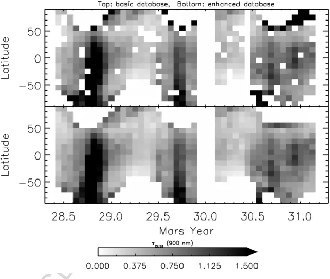
S) to generate the zonal dust climatology shown

in Figure 3. Here, the upper panel illustrates the basic retrievals binned as described while the lower panel includes the effects of additional filtering (e.g., outliers in a single bin, clipping the polar hood) and of interpolation to fill in the empty bins that are bracketed by “good” data. This database of optical depths is referenced to a wavelength of 900 nm and normalized to a surface elevation of 0 m, i.e., the aeroid. We calculate this normalization using the Mars Orbiter Laser Altimeter topography (Smith et al., 1999) and the assumption of an exponential atmosphere with a scale-height of 10 km. The uncertainty associated with the dust optical depth for an individual bin is estimated to be max(10%τdust, 0.1), which includes both the accuracy of

the retrieval process and the scatter associated with multiple retrievals points in the bin.

The values in Figure 3 are the result of an iterative process, where the dust optical depths (τdust) are derived ultimately by including the water

ice optical depth derived from contemporaneous MARCI observations; by default, every CRISM EPF should occur within a MARCI image swath). In other words, the dust column for each CRISM EPF observation is initially computed under the assumption of no water ice. This set of dust columns was used to create the initial version of the dust climatology employed to retrieve water ice optical depths from MARCI images for the period of November 2006 through December 2011. The resulting MARCI τice values associated with

each EPF spatial footprint are then used as an input in the next iteration of the CRISM EPF retrieval. This sequence was repeated three times, at which time there is essentially no change observed in either τdust or τicein the third

ACCEPTED MANUSCRIPT

Figure 3: CRISM zonal-mean dust map. The top panel is the result of binning approx-imately 24000 dust optical depth retrievals using a zonal scheme with widths of 10◦ _in

latitude and 22.5◦_{in LS. The bottom panel includes the effects of additional filtering for}

bad retrievals and of interpolation to fill in empty bins. The optical depths are defined at a wavelength of 900 nm and normalized to an altitude of 0 meters. The gap centered around the start of Mars Year 30 represents the extended spacecraft “safing” event in the latter part of 2009.

ACCEPTED MANUSCRIPT

3. Retrieval Algorithms and Methodology

The actual transformation of the MARCI Band 7 observations from ra-diance to τice is a direct and efficient computational task. By fixing the

other input parameters and exploiting the monotonic nature of adding a very bright scatterer above a dark surface, the deriviation of τice does not

need to involve the traditional non-linear approach. Instead, the process is a one-to-one mapping of radiance to τice. Furthermore, the use of a

multi-dimensional lookup table (LUT) and standard interpolation techniques allow one to dispense with computationally inefficient “live” calls to a multiple-scattering radiative transfer code. In this section, we provide an overview of the retrieval algorithm from the initial data processing step through the τice

retrieval. This is followed by a description of the LUT and the various input parameters that represent the “physics” of the atmospheric state vector and the boundary conditions.

3.1. Retrieval Procedure

The methodology by which the MARCI observations are converted from raw 8-bit data number (DN) values to a water ice optical depth consists of several discrete steps. Although the cadence of MRO orbit and the terrestrial day provides for the natural grouping of the 12-13 swaths of images per day as a “mapping day,” we treat a single MARCI image (or swath) as the basic unit for the processing algorithms.

1. Generation of radiometrically calibrated images. The procedure for taking MARCI raw 8-bit DN data (i.e., Level 0 Experiment Data

ACCEPTED MANUSCRIPT

Records) to calibrated radiance is well described by Bell et al. (2009). Although we implement these processing steps using an IDL-based set calibration routines, the United States Geological Service’s ISIS 3 soft-ware replicates this capability with its MARCICAL tool. Here, we include the additional step of removing the dependence of the observed radiance on solar distance by normalizing the data to incident solar ra-diance. The resulting quantity is the so-called I/F or radiance factor, as defined by Hapke (2012, p. 264). Specifically, I is the observed radi-ance, and F is the radiance that would be observed for a perfect Lam-bert surface illuminated normally by the top-of-the-atmosphere solar flux (J): F = J/π. The Mars-Sun distance is calculated for the rele-vant spacecraft clock time from the MRO and Mars SCLK (spacecraft clock) and PCK (planetary constants) kernels. These data files and core SPICE software libraries are distributed by NASA’s Navigation and Ancillary Information Facility (NAIF).

2. Geographic, Photometric, and Reflectance Information. For each pixel in a given image, we calculate the photometric angles (incidence, emer-gence, and phase) and location information (latitude, longitude). The elevation of the surface is taken explicitly into account for these calcula-tions using the Mars Orbiter Laser Altimeter (MOLA) derived products (i.e., Smith et al., 1999, ; see also http://pds-geosciences.wustl. edu/missions/mgs/mola.html). Finally, a surface reflectance model value (the w parameter decribed later) is assigned to each pixel using the Band 7 map product discussed below in Section 3.4.

ACCEPTED MANUSCRIPT

3. Dust column (τdust) and surface pressure (Psurf). These two quantities

are derived from the CRISM zonal optical depth database discussed in Section 2.2 and from a surface pressure field calculated by the Ames GCM (Smith, 2004). Specifically, we set the τdust and Psurf for the set

of nadir pixels in each MARCI image, with the cross-track pixel values populated using the MOLA surface elevations and the assumptions of uniform vertical mixing (with respect to gas density) in an exponential atmosphere with scale height of 10 km for both gas and dust. The nadir τdust are interpolated in latitude and LS from the CRISM climatology.

4. At this point, we have specified six of the seven variables in the LUT described in 3.2 and listed in Table 2. It is now a simple process to derive τice for each pixel through interpolation. A pixel mask is

also created to reflect any parameter value (for a given pixel) that is outside of the ranges in the LUT. A common example of this would be for emergence or incidence angles being too large. In addition to diagnostic information, the mask is used to discriminate between τice=0

due to the absence of clouds caused by an input parameter out of range. Figure 4 shows an example of a calibrated I/F image from a northern summer solstice observation and the resulting τice image.

5. Surface Ice Flag. The retrieval cannot practically distinguish between surface and atmospheric ice. In our implementation, we assume that any radiance needed above the τice=0 case (after all other dimensions

are fixed) must be provided by atmospheric water ice above a non-icy surface. As a result, an attempt to flag potential surface ice pixels occurs necessarily in a post-processing step. As can be seen in Figure 4,

ACCEPTED MANUSCRIPT

Figure 4: An example I/F image and the resulting τice product that includes part of the

Tharsis ridge near northern solstice in MY 33. The longitude of the nadir point at the equator crossing is 236◦ _{E. The ranges of latitudes starts near -45}◦ _{on the left side of the}

imaging, passes over the pole and ends near 60◦ _{N. The images are oriented such that}

North is to the right and West is up. This figure also demonstrates the retrieval limitation associated with surface ice, suggesting the utility of a post-processing step to identify pixels that are likely to include surface ice. See text.

ACCEPTED MANUSCRIPT

thick clouds are “derived” for pixels within the north polar residual cap and outliers. However, one might also notice that in addition to the proximity to the north pole, these pixels are quite bright in I/F compared to those of the more diffuse cloud features. We combine these these aspects, location and brightness, into a set of criteria for flagging potential surface ice.

In terms of location, we use the polar cap regression analysis of Can-tor et al. (2010) for the north polar region, as well as a similar unpub-lished analysis for the south cap. We flag a pixel as potentially including surface ice if it is poleward of the notional cap edges as defined below:

latN = 59◦ + 0.214 LS− C, 0◦ ≤ LS ≤ 90◦ latN = 59◦ + 0.214 (180◦− LS) − C, 90◦ ≤ LS ≤ 180◦ latN = 59◦, otherwise. latS = −12◦ − 0.247 LS, 180◦≤ LS ≤ 270◦ latS = −12◦ − 0.247 (540◦− LS), 270◦ ≤ LS ≤ 360◦ latS = −57◦, otherwise,

where latS and latN are the latitudes of the southern and northern cap

edges, respectively. The offset C compensates for the fact that the original regression formulae were designed to track the seasonal cap. However, not all of the outliers in the north polar region are inside the boundaries defined. For example, the southern most outliers in the Figure 4 are ∼2-3◦ _{southward of the notional boundary of 78}◦_.

ACCEPTED MANUSCRIPT

Given that this is an extrema case, it suggests a definition of C = 3 for 72◦ _{< L}

S < 108◦. Otherwise, C = 0.

In addition to the latitude, the effective reflectance of a pixel is a use-ful parameter. That is to say, we also set a threshold Lambert Albedo (AL) that must be exceeded for a pixel to be flagged as potential surface

ice. The albedo of outliers, as determined directly from the observed radiance (AL = (I/F )/(cos i)), is generally >∼0.12-0.15; whereas that

of the more diffuse structure (i.e., cloud) just south (left) and north (right) of the southern outliers in Figure 4— is ∼ 0.05 − 0.06 (associ-ated τice ∼ 0.1). For automated processing and image binning, a more

conservative threshold of 0.04-0.06 would be recommended. However, for maximum flexibility, we create a set of flags which indicate a po-tential surface ice detection for a family of threshold values, e.g., 0.04, and 0.06, and 0.08, For the results presented in this paper, we adopt a conservative threshold of 0.04 to minimize the contamination of the results with surface ice. However, we emphasize that our methodology only creates a mask or a flag; any water ice clouds in the polar region (above a non-icy surface) are still retrieved and tabulated.

3.2. Look-up Tables and Interpolation

The use of a LUT is motivated by the significant increase in performance compared to that for “live” or direct calls to a multiple-scattering radiative transfer (RT) routine. A single MARCI UV image (one orbital swath) typi-cally contains more than 300,000 pixels of valid data (i.e., photometric angles within acceptable range, etc.). Even with a notional processing time of 0.5 second per pixel, it would take more than a day to perform the RT for a single

ACCEPTED MANUSCRIPT

image (recall that there are typically 13 images per mapping day). In con-trast, the approach of LUT-and-interpolation requires less than one minute for the same number of pixels using a Fortran-based implementation (com-piled with gfortran and executed on a single core of circa-2012 MacPro). Of course, the computational efficiency does come with a potential cost, namely some loss of numerical accuracy due to the linear interpolation.

The error associated with interpolation may be reduced by increasing ei-ther the sophistication of the interpolation scheme (e.g., cubic spline versus linear interpolation) or the sampling frequency of the underlying function. While the function that we wish to interpolate is six-dimensional and gen-erally non-linear, we are not limited in how the function is sampled. After some numerical experimentation with higher order interpolation routines and non-linear sampling of each dimension of the LUT, we ultimately chose a lin-ear interpolation scheme with an increased sampling frequency (including a non-linear grid for several axes). With modern computers and sophisticated RAM caching techniques used in UNIX-based operating systems, the addi-tional computation cost of a larger LUT is less than that for a higher order interpolation algorithm. In other words, we increase the number of sample points for each the input variables and choose a mesh to allow for (quasi-) linear behavior of the radiance between the grid points.

A general goal in the above optimization of the LUT and the algorithm choice was to keep the maximum deviation between interpolated and exact results below 1%. In addition, the choice of specific tessellation for a given input parameter is the direct result of the sensitivity of the model radiance to that particular parameter and the limitation of a linear algorithm to represent

ACCEPTED MANUSCRIPT

Table 2: Water Ice Retrieval LUT Content

Parameter Number of Points Range of Values Mesh

Emergence angle (e) 15 0◦_-70◦ _linear

Incidence angle (i) 9 0◦_-80◦ _{linear in cosine of angle}

Azimuth angle (φ) 31 0◦_-180◦ _linear

Hapke w 8 0.05-0.12 linear

Surface pressure (Psurf) 7 0.3-13.3 (mbar) linear

Dust optical depth (τd) 10 0.01-3.01 non-lineara

Ice optical depth (τi) 23 0.0-4.0 linear

a

τd nodes: 0.01, 0.10, 0.25, 0.50, 0.80, 1.20, 1.65, 2.11, 2.56, 3.01

that functional dependence. For example, one can demonstrate that a coarser sampling is possible for surface pressure or surface reflectance as compared to photometric angles. In general, a linear mesh tends to work well, but we are able to gain some savings in LUT size by using a non-linear sampling for the dust optical depth; bringing the size from 1.4 GB to 200 MB without any noticeable increase in interpolation error. The smaller size decreases the read-in time of the LUT by more than 70%. Similar efforts for the water ice optical depth do not yield a corresponding improvement, so we stay with a conservative sampling scheme. The final parameter sampling details for the LUT are listed in Table 2.

The interpolation and sampling error associated with a given parameter mesh is quantified using a basic monte carlo experiment. Under the assump-tion of a uniform distribuassump-tion for the photometric angles and the Hapke w

ACCEPTED MANUSCRIPT

parameter, we (randomly) sample 7 values for each of these parameters using the ranges specified in Table 2, and combine these 7 uniformly spaced values for both τdust and τice (ranges also from the table). After choosing a typical

surface pressure of 6.1 mb, the normalized radiance (or radiance factor, I/F; see below) is calculated for this set of 117649 parameter combinations using both LUT and direct radiative transfer calculations. Each set of calculations is performed using the same atmospheric and aerosol properties. We then assessed the distribution of fractional error in radiance against our goal of ∼ 1%. The result of this exercise is the selection of the ultimate LUT, which balances data volume and interpolation error. The LUT described by Table 2 is used to generate the results shown in Figure 5. 98% of the models having an interpolation error of less than 1%, while of the models have errors less than 2%.

3.3. Radiative Transfer Algorithm

We perform the radiative transfer calculations needed to construct the LUT using the public-domain package DISORT (DIscrete ORdinate Radia-tive Transfer; Stamnes et al., 1988; Thomas and Stamnes, 2002). The “front-end” model atmosphere is that described by W10, which includes the CO2

-specific Rayleigh scattering cross sections of Sneep and Ubachs (2005) and Ityaksov et al. (2008). For the calculations presented here, we utilize sixteen streams (N = 8 ordinate pairs), and 128 terms in the Legendre polynomial expansion for the dust and water ice phase functions. This number of terms is that needed to get a good representation of each of the phase functions, as is required for the Nakajima and Tanaka intensity correction (i.e., Laszlo et al., 2010; Stamnes et al., 1988; Lin et al., 2015).

ACCEPTED MANUSCRIPT

−0.02 −0.01 0.00 0.01 0.02 interpolation fractional error 0

5000 10000 15000

number of models

Figure 5: Histogram of the fractional error in radiance for the interpolation algorithm and LUT adopted for this study. The mean error of the 117,649 models is 0.13% and the standard deviation is 0.3%. Perhaps more significantly, 98% of the models have an error less than 1% and 99.99% have an error less than 2%. See text for more details.

ACCEPTED MANUSCRIPT

Initially, we adopted the surface reflectance prescription of W10, a tradi-tional “Hapke function” (e.g., Hapke, 1993, Chapter 12) whose parameters did not vary spatially. The limited nature of the data analyzed by W10 -nearby the two Mars Exploration Rover sites and generally very dusty atmo-spheric conditions – may have minimized the need for a more complex treat-ment. However, during the early stages of the cloud mapping retrieval devel-opment, it was determined that the surface phase function needs to be more forward-scattering to avoid artifacts particularly apparent at larger phase an-gles (i.e., high latitudes). This type of effect concerns the five Hapke function parameters associated with the angular distribution of the reflectance: b, c, ¯θ, B0, and h. Using the symbol definitions of Johnson et al. (2006a,b), these are

the asymmetry parameter, the backward scattering fraction, the macroscopic roughness, the opposition effect width, and the opposition effect amplitude, respectively. In addition, a second set of artifacts were noticed for images with little or no water ice opacity. The fact that this latter set of features seemed to correspond to traditional bright and dark regions suggested that the need for some spatial-variability in the model, such as in the Hapke w parameter (the single scattering albedo of the surface). We approach both issues through numerical experimentation.

Improvements in the surface phase function (i.e., set of 5 Hapke param-eters) were performed through the repeated application of the cloud optical depth retrieval algorithm (as well as that for ozone, e.g., to adjust the Band 6 phase function, Clancy et al. (2016)) to regions where the surface artifacts were observed, but under conditions of minimal aerosol content. Specifically,

ACCEPTED MANUSCRIPT

we use observations at high southern latitudes during southern summer where topographic variation correlates strongly with phase angle, but also low dust and water ice columns; discrete dust events were excluded using the MARCI visible bands. In this manner, one is able to isolate the effects of the sur-face reflectance model. Briefly, we employ multiple overlapping images for each experiment and the requirement is that the surface phase function must produce spatially consistent w values. Iteration on the Hapke parameters is done manually (i.e., “chi-by-eye”), though automation is used to generate a range of candidate parameter sets to provide the analog of the Jacobian ma-trix for each iteration. The final parameter set is the result of approximately 10 experiments per band. The resulting more forward-scattering surface phase function is found to eliminate artifacts without introducing issues else-where in the dataset (e.g., at low and middle latitudes). The ultimate set of spatially-constant Hapke parameters is b=0.30, c=0.70, ¯θ=20◦_{, B}

0=1.0, and

h=0.06 (W10 differ in their c=0.45 and B0=0.8). Since our analyses using

both UV bands does not clearly require a wavelength dependence, we adopt a single set of these five values; as will be seen below, spatial variability will be limited to the w parameter. The new surface phase function does result in an effective change of the mean Hapke w values of 0.07 and 0.095 in W10 for Band 6 and 7, respectively, to those of 0.057 and 0.078. The corresponding normal Lambert (AL) reflectance values for the near-nadir regions become

0.014 and 0.017, respectively (versus the previous values of 0.011 and 0.014, respectively).

The second type of artifact suggested the need for spatially dependent Hapke w parameters The process involved in this improvement is more

com-ACCEPTED MANUSCRIPT

plicated, which we describe in Appendix A. For now, we summarize the resulting product with Figures 6 and 7. The first figure displays the spa-tial dependence of the surface reflectance for Band 7. Although the map clearly contains noise at the scale of a few degrees, there are correlations of UV “bright” regional features with traditional low albedo features such as Syrtis Major, Acidalia Planitia, and Margaritifer Terra. This is a manifesta-tion of the so-called “ultraviolet reversal” previously identified using Viking and Hubble Space Telescope observations (e.g., Thomas and Veverka, 1986; Bell and Ansty, 2007). While such efforts typically focus on smaller spatial scales, they did not include a radiative transfer-based analysis to disentangle the amplitude and spatial-extent of the effect, as illustrated in our map.

Figure 7 highlights the distribution of the w values and its relationship to the mean w value described above. The similar shape of the distribution for each of two channels is not coincidental. The intrinsically lower surface reflectance and the increased relative contribution of atmospheric scattering in Band 6 make intractable the derivation of map of similar quality to that in Figure 6. In the end, to get the Band 6 values used by Clancy et al. (2016)), we simply scale the Band 7 results by the ratio of the mean w values derived from earlier experimentation, mentioned previously.

As discussed above, we do not explicitly treat the surface reflectance of ice since the MARCI data cannot effectively discriminate between surface and atmospheric ice. As a result, a retrieval over an icy surface uses the bare surface reflectance calculated using Figure 6 and the other associated Hapke parameters. Although an effort is made to identify these cases after the fact (i.e., pixel mask), any radiance associated surface ice will be mistakenly

ACCEPTED MANUSCRIPT

Figure 6: Map of Band 7 Hapke w. The resulting spatial dependence of the Hapke w parameter derived using the procedure discussed in Appendix A. This map provides the spatial dependence of the surface reflectance input for the ice optical depth retrieval algorithm.

ACCEPTED MANUSCRIPT

Figure 7: Histogram of the Band 6 and 7 Hapke w Maps. The distribution of w values for Band 6 (solid line) and 7 (dashed line) resulting from the process described in Appendix A. The mean Hapke w values in the text are shown by the vertical solid (0.057) and dashed (0.078) lines for Bands 6 and 7.

interpreted as that due to atmospheric water ice opacity.

As a closing note on this topic, our goal is to provide a function that is adequate for use as a surface boundary condition in atmospheric retrievals. Accordingly, our results require a few caveats to keep in mind. Firstly, the five surface phase function parameters (b, c, ¯θ, B0, and h) are assumed to be

spatially constant, with the needed variability contained in the w parameter. Anecdotal evidence for this may be found in the fact that if one re-performs the optical depth retrievals near the MER locations at low and moderate dust loading by Wolff et al. (2009), but switching the Hapke phase function parameters (i.e., MER-A becomes MER-B and vice versa), one finds optical depths and w values that are generally consistent (ı.e., within the error bars) with those derived from the original values. Next, we assume that there is

ACCEPTED MANUSCRIPT

no seasonal component to the surface properties; namely, the w values are the same for all LS. So, temporal variability of surface features as a result

of aerolian processes will introduce an error into the retrieval. Finally, we derive values with eye towards minimizing artifacts in the retrieval products that appear to be associated with the surface model. As will be seen in the error analysis presented later (§ 4.1.1), even a 20% error in the surface reflectance has a minimal effect on the retrieved optical depth. This relative insensitivity is directly due to the contrast of bright clouds with the dark nature of the surface in the UV. As a result, the effort that would be needed to derive robust surface parameter uncertainties is deemed outside the scope of this paper, and we leave such efforts for future work.

3.5. Dust Aerosol Model

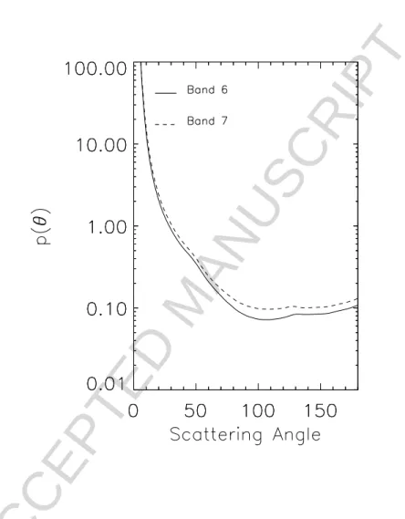
We specify UV dust radiative properties using the model presented by W10, which is derived from MARCI UV observations during the 2007 (MY 28) global dust event. We calculate dust properties appropriate for diffuse loading conditions using a gamma distribution with moments ref f=1.5 µm

and vef f = 0.3 (for definitions, cf. Hansen and Travis, 1974). Following

W10, the individual particle properties are calculated using the T-Matrix algorithm (e.g., Mishchenko et al., 2002) assuming a cylindrical particle with a diameter-to-length ratio (D/L) of 1. Figure 8 shows the resulting single scattering phase functions, including the empirical correction of W10. The effective single scattering albedo values for Band 6 (260 nm) and Band 7 (320 nm) are 0.64 and 0.68, respectively. The ratio of extinction cross sections rela-tive to 900 nm are: τBand6/τ900nm = 0.89 and τBand7/τ900nm = 0.90. Although

ACCEPTED MANUSCRIPT

the refractive indices taken from W10; the same as used here. They actually use the same size distribution moments as here, i.e., a column-integrated average of ref f=1.5 µm. Finally, we adopt a constant mixing ratio with

re-spect to the gas density for the dust vertical distribution and the same size distribution for all heights.

3.6. Water Ice Aerosol Model

Due to the complexity associated with attempting to use spatially-variable water ice particle properties, we restrict ourselves to a single set of physical characteristics and associated radiative properties. In order to “split the dif-ference” between properties found in the aphelion cloud belt, mid-latitudes, and (sun-lit) polar hood regions, we adopt a size distribution described by the moments ref f = 3.0 µm and vef f = 0.1, using a functional dependence

spec-ified by a gamma distribution. Because we are dealing with only a limited wavelength regime, the primary impact on the retrieval of different particle sizes would be seen primarily in the amplitude of the phase function in the side- and back-scattering directions. As will be discussed later (§ 4.1.2), it is difficult to quantify the result of different particle sizes for our retrieval. The vertical profile is set using a cloud bottom of 15 km and a constant volume mixing ratio (with respect to gas density) above this altitude. As can be found in a literature review (e.g., Clancy et al., 2017, Table 5.1), these values are not unreasonable, particularly given the desire for simplicity (and repro-ducibility by others) inherent in using a single size distribution to represent a vertical column of water ice particles. Since we use only a single MARCI band (Band 7; Band 6 is included to document details cited by Clancy et al. (2016)), a mismatch between the model and the actual size distribution (for

ACCEPTED MANUSCRIPT

Figure 8: Adopted dust phase functions for Band 6 and 7. The T-Matrix calculations for D/L=1 cylinders (with ref f = 1.5 µm and vef f=0.3) are modified as described by W10.

ACCEPTED MANUSCRIPT

a given pixel) would impact the derived optical depth through the water ice phase function, i.e., no change in the single scattering albedo of water ice.

With a refractive index of 1.34+2.0 × 10−9_{i at 260 nm and of 1.33+2.0 ×}

10−9_{i at 320 nm (e.g., Warren and Brandt, 2008), the single scattering albedo}

is unity for both bands, regardless of particle shape. In terms of wavelength dependence, we use Band 7 as the reference point for the ice optical depth, but the ratio of extinction cross sections for the two bands is also essentially unity (to a precision better than 1%).

The final radiative property needed is that of the scattering phase func-tion. Unfortunately, Mars water ice phase function models are appreciably less mature than those for Mars dust aerosols. Crystal habits found for terrestrial cirrus particles (e.g., hexagonal prisms) have not been particu-larly helpful for Martian applications (e.g., Clancy et al., 2003). Fortunately, terrestrial analogs for Martian atmospheric conditions (temperature, super-saturation) suggest a more useful shape, namely an incomplete crystal habit referred to as polycrystalline or, in one realization as a “droxtal” (e.g., Thu-man and Robinson, 1954; Ohtake, 1970; Baker and Lawson, 2006; Bailey and Hallett, 2009). As described in Appendix B, we adopt the droxtal shape and employ a combination of first principles scattering calculations and empirical adjustment. The resulting phase function is displayed in Figure 9, where it is compared to those for an average of the empirically derived phase phase functions by Clancy et al. (2003), for a distribution of equivalent spherical particles, and for two Henyey-Greenstein phase functions using the asymme-try parameter value of 0.7 adopted by Mateshvili et al. (2007) and that for an equivalent sphere calculation (0.84, ref f=3 µm).

ACCEPTED MANUSCRIPT

Figure 9: Adopted droxtal-based water ice aerosol phase functions for Band 7. It is compared to the phase functions for an average derived by Clancy et al. (2003, Figure 10) (one type 1, two Type 2), for a distribution of equivalent spheres, and for a Henyey-Greenstein function with asymmetry parameters of 0.7 (e.g., Mateshvili et al., 2007) and 0.84 (equivalent sphere calculation).

ACCEPTED MANUSCRIPT

4.1. Water ice optical depth images and associated uncertainties

The process described in section 3.1 produces a set of water ice optical depths in the form of an image, having the same shape and covering the same physical area as the original MARCI observation. In other words, the radiance values are replaced by the corresponding retrieval result; see the lower panel of Figure 4. The image masks (as discussed in 3.1) are also rendered in a similar format. One mask contains information about the potential inclusion of surface ice, while the other encodes information about the success (or failure) of the retrieval for that particular pixel. An advantage of retaining the image geometry/format is that the τiceproducts can be easily

projected onto any desired coordinate system using the geometry information associated with the original MARCI image. This is likewise true for any of the metadata values, e.g., photometric angles. An example of this capability is shown in Figure 10, where a mapping day from the aphelion cloud belt period (i.e., 01-January-2016) is projected onto a cylindrical grid.

4.1.1. General Retrieval Uncertainties

Excluding the possible issue of water ice particle size (ref f) as manifested

through the water ice particle phase function (we will return to it below), the uncertainties associated with the MARCI τice dataset are dominated by

several model input parameters and the radiometric calibration. Because the pointing registration and camera model have been validated against the MARCI observations at native (∼1 km) resolution using data taken center of the optical axis (i.e., Band 3), we treat the errors associated with the

ACCEPTED MANUSCRIPT

Figure 10: Map-projection of one mapping day of τice retrievals. The water ice cloud

re-trievals from 01-January-2016 (MY=33, LS=89.1◦) are shown in a cylindrical map

projec-tion. The high latitudes are omitted to minimize surface ice confusion in this presentaprojec-tion. See text.

ACCEPTED MANUSCRIPT

photometric angles as negligible. We list the remaining relevant sources in Table 3. The first three rows give conservative uncertainty estimates for the specific parameters (τdust, surface pressure and surface reflectance) derived

from the perturbation analysis described in the Appendix C. The first column represents an average error, while the second is a measure of the spatial variability within an image strip.

The fourth and fifth lines in Table 3 give different estimates of the to-tal error associated with the three model inputs. The former assumes an uncorrelated behavior between the terms, which tends to capture the mean behavior. The second estimate attempts to include the effects of variability through a simple monte carlo analysis described in Appendix C. This in-volves representing the individual error terms as Gaussian distributions and sampling them over a comprehensive range of ice optical depths. The larger value of the monte carlo-based estimate suggests that the variability of the errors within an image does contribute to a larger total error. This is in contrast to the case of the fixed error terms in the perturbation analysis.

We also need to consider the impact of errors associated with the data. We restrict our attention to the dominant source, the radiometric calibration, and repeat the above exercises to characterize the radiometric error term and to include it in the total error estimation (see Appendix C). The results may be found on lines 6-8 of Table 3. We adopt the larger of the two errors, giving ∆τice=0.03 as the uncertainty of the MARCI τice retrievals.

4.1.2. Retrieval Uncertainties from ref f, Phase Function

The uncertainty in the retrieved τicerelated the adopted ref f is associated

ACCEPTED MANUSCRIPT

Table 3: Water Ice Optical Depth (τice) Uncertainties

(exclud-ing ice ref f effects)f

Error Source ∆τ¯ice σ∆τa

τdust (±20%) ±0.003 0.009

Hapke w (±20%) ±0.010 0.007

Surface Pressure (±10%) +0.005,-0.009 0.004 TotalABOV E (uncorrelated)b +0.014,-0.012 . . .

TotalABOV E (monte carlo) c ±0.019 0.002

Radiance (±7%) ±0.017 0.005

TotalALL (uncorrelated)d +0.022,-0.021 . . .

TotalALL (monte carlo) e ±0.029 0.003

a _{The standard deviation is the square-root of the mean of}

the variances from both perturbations.

b

Error from the above three sources are added in quadrature assuming no correlation.

c

Error from the above three sources, but sampled using monte carlo. See text.

d

Error from all four sources are added in quadrature assum-ing no correlation.

e _{Error from all four sources, but sampled using monte carlo.}

See text.

f _{As described in 4.1.2, the retrieved τ is estimated to}

be ∼30-40% too high if the clouds have particles with ref f=1.5 µm, but only slightly lower (less than 10%) for

ACCEPTED MANUSCRIPT

reality. This dependence is a fundamental limitation or uncertainty inherent in scattering retrievals. As seen in Figure 9, the relative difference between various phase functions can be quite large, in particular when considering in-appropriate cases (e.g., spheres, Henyey-Greenstein). For example, repeating the perturbation experiments of the previous section but this time switching the phase function, one sees relative changes that generally correlate directly with the relative differences in Figure 9. This would be expected if single scattering were dominating the observed radiance. However, before becoming too alarmed by the huge differences at some scattering angles, it is important to recall that we are comparing our model to some very inapplicable phase functions.

Of course, it is challenging to know what is more appropriate. This is particularly true for Martian water ice aerosols, which have not been exam-ined and tested in the same way as dust aerosols (e.g., Wolff et al., 2017, and reference within). While we have endeavored to include as much phys-ical reality in our phase function derivation (Appendix B), one must keep in mind this sensitivity to the adopted phase function. At a minimum, our efforts have yielded some degree of confidence with the shape of the water ice phase function.

Nevertheless, if we assume our model is not horribly wrong, we can es-timate the impact of particle size on the MARCI optical depths. Assuming that the relative change in the opacity is dominated by single scattering ef-fects, we can use phase function ratios. We employ droxtal calculations to calculate for ref f <3 µm but need to use spheres for larger ref f. Averaging

ACCEPTED MANUSCRIPT

retrieval (assuming ref f= 3 µm) could over-estimate the optical depth by

∼30-40% if the actual ref f is 1.5 µm, while slightly under-estimating ( <

∼10% ) for larger (4-6 µm). Finally, unless one expects that the column-integrated particle sizes are changing from pixel-to-pixel, this type of uncertainty will tend to apply for comparisons between different regions and seasons where the microphysical processes are sufficiently different.

4.2. Constructing a database of retrievals

The MARCI τice retrieval process generates a significant amount of data,

especially when one considers the months and years of data that one might wish to analyze. For example, the 1-January-2016 observations that are shown in Figure 10 produce 60 MB of data (τice and associated metadata

fields), even when stored as (gzip) compressed, scaled two-byte integers. This data volume per day leads to about 220 GB, from the beginning of mapping operations (in November 2006) until the end of September 2018. Clearly, any practical tabulation, analysis, or public data product involving multiple years of observations will require a binned product, i.e., temporally, spatially, or both.

For the purposes of the analyses and the discussions in this paper, we construct an 8x8 pixel (spatially) binned product; ∼ 1◦ _{per pixel at nadir.}

In addition to the bin-average photometric angles, we include latitude, lon-gitude, adopted τdust, ephemeris time (as a proxy for Mars Year and LS),

local true solar time (LTST; all times in this paper are LTST), surface ice pixel flag (described above), and some basic statistical information – number of original pixels in the bin (we only include retrieval pixels not flagged as possibly containing surface ice), the standard deviation about the mean for

ACCEPTED MANUSCRIPT

τiceand τdust. The size of the resulting data set – again stored as compressed

two-byte integers – is about 100 times smaller: ∼2 GB vs. ∼200 GB. There is an additional factor-of-two savings beyond that expected from the binning due to the net decrease in metadata compared to that originally produced.

5. Discussion

At present, the MARCI observations span six Martian years with system-atic spatial sampling, though with a limited local time coverage due to the sun-synchronous nature of the MRO orbit. For reference, the nadir LTST value for low latitudes is listed in Table 4, where the full width of the MARCI strip (assuming 65◦ _{emergence angle) changes from 1.3 (Martian) hours at}

below 30◦ _{in latitude to 2.4 hrs at 60}◦ _{and 2.6 hrs at 75}◦_{. With the large}

amount of data, it is natural to start with a global-scale view and then move to a more regional perspective. We begin with a zonally averaged view of the MARCI τice over multiple Mars Years. We then move to comparison

and discussion of other observations, continuing the focus on zonal mean behavior but also including some temporally-binned zonal-meridional (i.e., latitude-longitude) products. For the latter, we limit comparison and discus-sion to TES data. Finally, comparisons will be made with the results from two GCMs. The theme of these discussions is to highlight the broad areas of agreement and disagreement with other observations and with model data. Such a set of exercises can potentially reveal useful information about sys-tematic issues between data sets, including MARCI (e.g., sampling, retrieval assumptions). In addition, the inclusion of models can highlight both the successes and the potential needs for improvement.

ACCEPTED MANUSCRIPT

Table 4: Local True Solar Time at Nadir for MARCI Observations (45◦ _{S - 45}◦ _N)

LS mean LTSTa,b∆LTST (max-min)c,d

0◦ _{14h35 h015}

90◦ _{15h15 0h15}

180◦ _{15h50 0h20}

270◦ _{15h15 0h20}

a _{Mean LTST for emergence angles <2◦ at}

lati-tudes between 45◦ _{S and 45}◦ _{N, over MY}

28-34.

b

The full width of the MARCI strip (assuming 65◦ _{emergence angle) is about 1.3 (Martian)}

hours, i.e.±0h40. The full width increases to 2.4 hrs at 60◦ _{latitude and to 2.6 hrs at 75}◦_. c

difference in LTST between maximum and minimum values observed for LS over MY

28-34. In comparison, the standard deviation of the LTST is always less than 40% of this dif-ference (typically between 25-33%).

d _{Units are Martian hours, 24h per sol, Mars}

ACCEPTED MANUSCRIPT

A zonal representation of the MARCI τice values, as shown in Figure 11,

clearly reveals the presence and repeatability of two global-scale cloud forma-tions: the aphelion cloud belt (ACB) and the polar hood (PH) clouds. These phenomena have been previously identified from multiple data sets and dis-cussed by several authors, as recently summarized by Clancy et al. (2017). However, the power of the MARCI data set is to be found in the consistency of the global (spatial) coverage across the extended period of time. When displayed in this way, the general behavior of the cloud optical depths seems remarkably consistent from year to year. Nevertheless, the eye does pick out some variations in the detailed spatial extent and temporal evolution.

A simple way to look at internannual variability is to subtract the multi-year average value, which is calculated for each LS-latitude bin using a sample

from all available Mars Years (for that bin). The results of such an approach can be seen in Figure 12, where a positive value represents higher optical depth at a given time than the average and a negative value less optical depth than the average. Of course, the amount of zonal averaging tends to smooth out more extreme variations that occur at specific longitudes. From this perspective, the mid-amplitude scale colors (i.e., |∆τice| ∼ 0.03) can

be indicative of non-trivial interannual variations. The largest variations, indicated by the saturated red and dark blue colors, are associated with the polar hoods (PH) and the initiation/decay of the ACB.

Two other trends exist in Figure 12 that merit a brief mention. The first is the variation of cloudiness in the late northern winter season and early northern spring. The variability seems to occur at both northern and

ACCEPTED MANUSCRIPT

Figure 11: Zonal τicedata set for MY 28 LS=153◦- MY 34 LS=178◦. Each pixel represents

an average of all longitudes for the given 1◦ _{latitude bin. To provide the most complete}

temporal coverage, we also average over local times between 14h-16h LTST. Most of the polar hoods are excluded due a combination of surface ice flags and solar incidence angle constraints.

ACCEPTED MANUSCRIPT

Figure 12: Zonal Difference data set for MY 28 LS=153◦- MY 34 LS=178◦, local times

included 14h00-16h00 LTST. The multi-year mean value for each LS-latitude bin

(calcu-lated using the values from all MY for that bin) is subtracted from value at a given time, so positive means more clouds than average and negative fewer.

ACCEPTED MANUSCRIPT

southern latitudes. For example, there is significantly less cloud opacity at low latitudes in late MY 28 but more in late MY 29. Another example is the trend from less optical depth in early MY 30 and 31 to more in MY 31 and 32. The second trend is the general increase of optical depth at mid-and low-latitudes from MY 29 through MY 33 (mid-and perhaps into MY 34) -note the general shift of negative (blue) to positive (red) differences. So even with six Mars Years of data, it is difficult to say whether this second trend is significant or if it is potentially repeatable or periodic. There are no signs of a drift in the instrumental calibration. It is noteworthy, though speculative, to remind the reader that this trend is bracketed by occurrences of global dust events in MY 28 and MY 34.

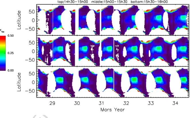
The LTST range in Figure 11 is chosen to provide relatively complete zonal-seasonal coverage; see Table 4 for image LTST range and seasonal change of nadir values. Although somewhat unanticipated because of the relative narrow window of local times, this averaging does in fact mask ap-preciable diurnal changes and associated interannual variations. For example, as can be seen in Figure 13, significant increases in the opacity of the ACB can occur within a one hour period from (14h30 to 15h30), but only in some Mars Years such as MY 30 and MY 31. This is in contrast to the changes between this period and the 15h30-16h00 interval, where the differences are generally more subtle and similar to those seen in Figure 11.

5.2. Comparisons with previous observations

Comparing observations from different instruments can be beneficial for a variety of reasons: extension of seasonal coverage (i.e., more Mars Years), interannual variability; extension of local time coverage (e.g., diurnal changes

ACCEPTED MANUSCRIPT

Figure 13: Local Time dependence of τice. MY 28 LS=153◦- MY 34 LS=178◦ for the

local time intervals 14h30-15h00, 15h00-15h30, and 15h30-16h00 LTST. The changes in the completeness of the coverage for various Mars Years is due to the changes in the orbit of MRO, including maneuvers to support other missions (Menon et al., 2017).

ACCEPTED MANUSCRIPT

of aerosol loading); verification of previously phenomena and validation of retrievals; and synergies in wavelength (e.g., particle size from visible and IR) and vertical resolution (combining column-integrated values with limb profiles). In this section, we are motivated by the first few items in the list, but we restrict our attention to column-integrated optical depths from data sets with systematic spatial sampling, at least in a mean zonal sense. In addition, we focus primarily on the mid- and the low-latitude behavior, e.g., the ACB.

5.2.1. Zonal - TES

We begin with Figure 14, an annual zonal mean comparison using TES re-trievals (from MY 24-25). The data set is described by Pearl et al. (2001) and Smith (2004). For comparison to MARCI, we use the publicly available TES water ice column-integrated absorption optical depth, which is referenced to 12.1 µm (1076 cm−1_{), kindly provided by M. Smith (personal}

communica-tion). Quantitative comparisons between these TES IR absorption optical depths and MARCI 320 nm extinction optical depths require the assump-tion of an ice particle size distribuassump-tion. Here we assume the same ice particle size distribution employed for the MARCI cloud retrieval LUT calculations, ref f=3 µm (vef f=0.1), In this case, the approximate ratio of the

MARCI-to-TES optical depth is 1.9. This number includes the cross section conversion of absorption to extinction and the scaling between 320 nm and 12.1 µm (i.e., Clancy et al., 2003; Wolff and Clancy, 2003). We incorporate this factor in Figure 14 by scaling range of the color bar similarly (i.e., 0.50/0.26 = 1.9), such that the same color in each panel would represent the same ice column abundance under the adopted water ice particle properties (ref f=3 µm).

ACCEPTED MANUSCRIPT

Figure 14: Multi-year mean zonal map comparison between MARCI and TES comparison. The MARCI data are extinction optical depths while those from TES are absorption optical depths. The MARCI data are averaged over the same range shown in Figure 12, both in season and local time. For TES, the average includes all valid daytime measurements (13h30-14h30 LTST). The TES “annual” data are taken from the interval that represents the highest quality data, namely MY 24 L =151◦_{- MY 25 L =151} ◦ _{(Smith, 2004, M.}

ACCEPTED MANUSCRIPT

A quick comparison between the two panels corroborates the general cor-respondance of the ACB and PH features in both data sets. However, there are some visual differences worth mentioning. In the case of the polar hoods, the lack of dependence on surface temperature for MARCI allows the re-trievals to extend to slightly higher latitudes than TES. On the other hand, the MARCI binning and surface ice flagging algorithm tend to remove all pixels inside the outer edge of the polar caps, including those pixels over bare surfaces. This gives TES more apparent high latitude coverage in the summer poles. So, these differences are simply a mismatch in the effective coverage between the two data sets.

A second difference is associated with structure of the ACB. From MARCI, it appears that the ACB is forming later in the season than observed from TES. However, taking into account the specific color scales (see above), the ACB in each data set actually persists for essentially the same duration, LS

∼ 60◦_-160◦_{. Rather, it is the shape or profile of the ACB (versus L}

S) that is

actually distinct between the two data sets. Specifically, MARCI and TES have similar ACB optical depths from 50◦_-60◦ _{until 75}◦_-80◦_{(as presented,}

ex-tinction @ 320 nm vs. absorption @ 12.1 µm). At this point, the MARCI τice

increase appreciably and remains relatively constant until the dissipation of the ACB. In effect, the TES ACB profile is approximately symmetric about LS= 90◦, while that for MARCI is skewed to later in the northern summer

season having a centroid near LS=120◦(see also Figure 28 from the GCM

comparisons in § 5.3).

These LS variations in the MARCI-to-TES optical depth ratio for the