HAL Id: hal-00699631
https://hal.archives-ouvertes.fr/hal-00699631
Submitted on 12 Jan 2017HAL is a multi-disciplinary open access
archive for the deposit and dissemination of sci-entific research documents, whether they are pub-lished or not. The documents may come from teaching and research institutions in France or abroad, or from public or private research centers.
L’archive ouverte pluridisciplinaire HAL, est destinée au dépôt et à la diffusion de documents scientifiques de niveau recherche, publiés ou non, émanant des établissements d’enseignement et de recherche français ou étrangers, des laboratoires publics ou privés.
Evolution Under Rainfall - Influence of Radar Precision
Richard Dusséaux, Edwige Vannier, Odile Taconet, G. Granet
To cite this version:
Richard Dusséaux, Edwige Vannier, Odile Taconet, G. Granet. Study of Backscatter Signature for Seedbed Surface Evolution Under Rainfall - Influence of Radar Precision. Progress In Electromagnetics Research, EMW Publishing, 2012, 125, pp.415-437. �10.2528/PIER11102807�. �hal-00699631�
STUDY OF BACKSCATTER SIGNATURE FOR SEEDBED SURFACE EVOLUTION UNDER RAINFALL — INFLU-ENCE OF RADAR PRECISION
R. Duss´eaux1, *, E. Vannier, O. Taconet, and G. Granet 1Universit´e de Versailles Saint-Quentin en Yvelines,
LATMOS/IPSL/CNRS, 11 Boulevard d’Alembert, Guyancourt 78280, France
2Universit´e Clermont-Ferrand II, Laboratoire des Sciences et
Mat´eriaux pour l’´electronique et d’Automatique (LASMEA), UMR 6602, BP 45, Aubi`ere 63177, France
Abstract—We propose a 3D-approach of the soil surface height variations, either for the roughness characterization by the mean of the bidimensional correlation function, or as input of a backscattering model. We consider plots of 50 cm by 50 cm and two states of roughness of seedbed surfaces: an initial state just after tillage and a second state corresponding to the soil roughness evolution under a rainfall event. We show from stereovision data that the studied surfaces can be modelled as isotropic Gaussian processes. We study the change of roughness parameters between the two states. To discuss the relevance of their differences, we find from Monte-Carlo simulations the bias and variance of estimator for each roughness parameters. We study the roughness and moisture combined influences upon the direct backscattering coefficients by means of an exact method based on Maxwell’s equations written in a nonorthogonal coordinate system and by averaging the scattering amplitudes over several realizations. We discuss results taking into account the numerical errors and the precision of radar. We show that the ability of the radar to discriminate the different states of seedbed surfaces is clearly linked to its precision. 1. INTRODUCTION
The interpretation of radar measurements in terms of soil roughness is a difficult task in view of the geometrical complexity of real soils
Received 28 October 2011, Accepted 5 December 2011, Scheduled 6 March 2012
and the influence of soil moisture. Electromagnetic simulations of radar signal are an essential step to understand the influence of such parameters on the backscattered signal. In this paper, we study the roughness and permittivity influence upon the backscattering coefficient by means of Monte-Carlo predictions. The backscattering coefficient is estimated by averaging the scattering amplitudes over several realizations. For each realization, the scattering amplitudes are obtained by the curvilinear coordinate method, commonly called the C-method [1–7]. This C-method is based on Maxwell’s equations under their tensorial form written in a nonorthogonal coordinate system where the boundary surfaces coincide with coordinate surfaces. As a result, the boundary value problem is simplified. Complexity is transferred to analytical expression of propagation equations. The C-method leads to eigenvalue systems. The scattered fields are expanded as linear combinations of eigensolutions satisfying the outgoing wave condition. The boundary value problem allows the scattering amplitudes to be determined. The C-method is an efficient theoretical tool for analyzing grating diffraction [1–3] and rough surfaces [4–7]. The method was investigated in near and far field zones by means of convergence tests on the scattering amplitudes and the power balance criterion. The theory was verified by comparisons with published numerical and experimental data [5–7]. We showed that the Monte-Carlo simulations based on the C-method have been successful in predicting backscattering enhancement and in analyzing very rough surfaces. The dominant computational cost for the C-method is the eigenvalue problem solution which is of the order of O(N3) where N
is the total number of unknowns. Owing to computational costs, the C-method does not allow analysing surfaces of very large sizes and surfaces with large correlation length. This is a weak point of the C-method. However, the strength of the C-method is that it leads to the eigensolutions of the scattering problem. It is an accurate method and it can be used as a reference for the analytical models. Nevertheless, as any numerical method, because the surface area and number of realizations have finite values and as the spatial resolution does not tend to zero, the average backscattering coefficient show numerical errors that must be quantified [8]. The C-method is described in Section 2.
In [9], a stereovision database of bare soil geometrical descriptions was presented. In the present paper, we consider plots of 50 cm by 50 cm associated with two roughness states of seedbed surfaces: an initial state just after tillage (state 1) and a second state corresponding to the soil roughness evolution after a rainfall event (state 2). In Section 3, we show that the studied soils with moderate roughness
and unmarked tillage patterns can be modelled as isotropic Gaussian processes. The autocorrelation function is defined by three roughness parameters: the root-mean-square height s, the length correlation l and the roughness exponent r [10, 11]. The Gaussian distribution is checked by the Kurtosis of the height data and the isotropy by the ratio of two directional correlation lengths computed in two perpendicular directions. The roughness parameters are estimated from the experimental autocorrelation obtained from stereovision data with a high millemetric spatial resolution. In Section 3, we also study the change of these parameters from state 1 to state 2 and we discuss the relevance of these changes.
In Section 4, for the different states of seedbed soils, we estimate the backscattering coefficients by the C-method. We study the roughness and moisture influences upon the backscattered signal. We discuss results taking into account the scattering model numerical errors and we study how the ability to differentiate these two seedbed surfaces of distinct roughness with different soil moisture evolution is related to the radar precision.
2. ANALYSIS WITH THE CURVILINEAR COORDINATE METHOD
2.1. Formulation of Problem
We consider a surface given by equation z = a(x, y), where a(x, y) is a local function defined over the surface area L × L. The structure is illuminated by a monochromatic plane wave with the wavelength λ. The time-dependence factor varies as exp(jωt), where ω is the angular frequency. Any vector function is represented by its associated complex vector function and the time factor is omitted. The surface separates the vacuum from a material with a complex relative permittivity. The incident wave vector ~k0 is defined from the zenith angle θ0 and the
azimuth angle ϕ0 [6, 7]. In horizontal polarization (a = h), the electric
field vector is parallel to the Oxy plane. In vertical polarization (a = v), this is the case for the magnetic field vector. For an incident wave in (a) polarization, in addition to incident, reflected and transmitted plane waves, we consider a scattered field ~Ed±(a)(x, y, z). The problem consists in working out the H-polarized component ~E(ha)d±
and the V -polarized component ~Ed±(va) of the scattered field. Subscripts (+) and (−) denote quantities relative to the upper medium and the lower medium, respectively.
2.2. Coordinate System — Covariant Components of Field The scattered field can be obtained by using the C-method [1–7] and the translation coordinate system defined by:
( x0 = x
y0 = y
z0 = z − a(x, y) (1)
In this coordinate system, the height function z = a(x, y) coincides with the coordinate surface z0 = 0. The change from Cartesian
components (vx; vy; vz) of a vector ~v to covariant components
(vx0; vy0; vz0) is given by [1]: vx0(x0; y0; z0) = vx(x ; y ; z) +∂a(x,y) ∂x vz(x ; y ; z) vy0(x0; y0; z0) = vy(x ; y ; z) +∂a(x,y) ∂y vz(x ; y ; z) vz0(x0; y0; z0) = vz(x ; y ; z) (2)
The covariant components vx0 and vy0 are parallel to the coordinate
surface z0 = z0. Consequently, the covariant components Ex0, Ey0, Hx0
and Hy0 are parallel to the rough surface and satisfy the boundary value
problem. Because the boundary surface coincides with a coordinate surface, the boundary value problem is simplified. Complexity is transferred to analytical expression of propagation equation.
2.3. Equation of Propagation in the Translation System In a source-free medium, from Maxwell’s equations and constitutive equations written in the translation system, we show that Ex0,±, Ey0,±,
Hx0,± and Hy0,± can be expressed in terms of Ez0,± and Hz0,± only [3]:
∂2E x0,± ∂z02 + k±2Ex0,± = ∂ 2E z0,± ∂x0∂z0 − k2±gx 0z0 Ez0,±− jk± µ gy0z0∂Z±Hz0,± ∂z0 + ∂Z±Hz0,± ∂y0 ¶ (3) ∂2E y0,± ∂z02 + k2±Ey0,± = ∂2Ez0,± ∂y0∂z0 − k 2 ±gy 0z0 Ez0,±+ jk± µ gx0z0∂Z±Hz0,± ∂z0 + ∂Z±Hz0,± ∂x0 ¶ (4) ∂2Hx0,± ∂z02 + k2±Hx0,± = ∂2Hz0,± ∂x0∂z0 − k 2 ±gx 0z0 Hz0,±+ jk± Z± µ gy0z0∂Ez0,± ∂z0 + ∂Ez0,± ∂y0 ¶ (5)
∂2H y0,± ∂z02 + k2±Hy0,± = ∂ 2H z0,± ∂y0∂z0 − k±2gy 0z0 Hz0,±− jk± Z± µ gx0z0∂Ez0,± ∂z0 + ∂Ez0,± ∂x0 ¶ (6)
Z± designate the impedances and k±, the wave numbers, respectively.
We also show that Ez0,± and Hz0,± obey to the same propagation
Equation (7): ∂2ψ ± ∂x02 + ∂2ψ ± ∂y02 + ∂2ψ ± ∂z02 + k 2 ±ψ± + ∂ ∂z0 " gx0z0∂ ψ± ∂x0 + ∂ gx0z0 ψ± ∂x0 + g y0z0∂ ψ± ∂y0 + ∂ gy0z0 ψ± ∂y0 # = 0 (7) where ψ± = Ez0,± in vertical polarization and ψ± = Z±Hz0,± in
horizontal polarization. Terms gx0z0
, gy0z0
and gz0z0
are elements of metric tensor which depend on the derivatives of function a(x0, y0) with
respect to x0 and y0 [3] gx0z0 = −∂a ∂x0 gy0z0 = −∂a ∂y0 gz0z0 = 1 + µ ∂a ∂x0 ¶2 + µ ∂a ∂y0 ¶2 (8) 2.4. Numerical Implementation
In previous works [6, 7], we proposed a procedure for solving the propagation Equation (7) in the spectral domain. We showed that the method requires the solutions of 2Ms-dimensional eigenvalue system
where Ms = (2M + 1)2 and M is the truncation order. The
Oz-components can be expanded as a linear combination of eigensolutions satisfying the outgoing wave condition.
ˆ ψd±(α, β, z0) = Ms X n=1 An,±ψˆn,±(α, β, z0) (9) ˆ
ψd±(α, β, z0) represents the Fourier transform of ψd±(x0, y0, z0).
According to the sampling theorem, we showed that the eigensolution ˆ
(eigenvector components) and eigenvalue rn,± by the following interpolations: ˆ ψn,±(α, β, z0) = exp(−jk+rn,±|z0|) × +M X p=−M +M X q=−M φn,±(αp, βq)sinc³ π∆α(α − αp) ´ sinc³ π ∆α(β − βq) ´ (10) where
αp = k+sin θ0cos ϕ0+ p∆α, βq= k+sin θ0sin ϕ0+ q∆α (11) The elementary wave function ˆψn,±(α, β, z0) represents an outgoing
wave travelling without attenuation if Re(rn,±) > 0 and Im(rn,±) = 0.
For an evanescent wave, Im(rn,±) < 0. We deduce from (3) to (6)
the H-polarized components of electric and magnetic fields ~Ed,±(ha) and
~
Hd,±(ha) by taking Ez0,± = 0 and the V -polarized components ~E(va)
d,± and
~
Hd,±(va)by taking Hz0,±= 0. For an incident wave in (a) polarization and
a scattered wave in (b) polarization, the amplitudes A(ba)n,± are found by solving the boundary value problem and a 2Ms-dimensional matrix
system.
Above the highest point of the surface, the scattered field can be represented by a superposition of a continuous spectrum of outgoing plane waves, the so-called Rayleigh integral [12]. In H-polarization, the Cartesian components of the electric field can be expressed as follows:
E+,x(ha)(x, y, z) = − 1 4π2 +∞ Z −∞ +∞ Z −∞ β p α2+β2Rˆ (ha) + (α, β) exp(−jαx−jβy−jγ+z) dα dβ ~ E+,y(ha)(x, y, z) = 1 4π2 +∞ Z −∞ +∞ Z −∞ α p α2+β2Rˆ (ha) + (α, β) exp (−jαx−jβy−jγ+z) dα dβ (12) where α2 + β2 + γ2
+ = k+2 and Im(γ+) ≤ 0. Substituting ~E+(ha) by Z+H~+(va) into (12), we obtain the V -polarized components of magnetic
vector. Functions ˆR(ba)+ represent the scattering amplitudes. We can write continuity relations between the transverse components of the Rayleigh expansion and the covariant components (3)–(6). For an
incident wave in (a) polarization, we deduce from continuity relations the scattering amplitudes ˆR(ha)+ (α, β) and ˆR+(va)(α, β) [5–7].
For an incident wave in (a) polarization and a scattered wave in (b) polarization, the average bistatic scattering coefficient σ+(ba)(θ, ϕ) in the upper medium is derived from the scattering amplitude ˆR(ba)+ (α, β) as follows:
σ+(ba) = cos2θ
λ2L2cos θ0 <
¯ ¯
¯ ˆR(ba)+ (k+sin θ cos ϕ; k+sin θ sin ϕ) ¯ ¯
¯2 > (13) where α = k+sin θ cos ϕ and β = k+sin θ cos ϕ. Angle θ designates
the zenith angle and ϕ, the azimuth angle, respectively. The angular brackets hi stand for an ensemble average. The average bistatic scattering coefficient is estimated by results over NR realizations.
In this paper, we only study the roughness and permittivity influence upon the backscattering coefficient corresponding to σ0(ba) =
σ+(ba)(−θ0, ϕ0).
In this section, we have succinctly presented numerical implemen-tation of the C-method. We refer the reader to references [4, 5] for more information on analysing one-dimensional rough surfaces and to references [6, 7] for analyzing two-dimensional surfaces.
2.5. Spectral Resolution and Spatial Resolution
The truncation order M and the spectral resolution ∆α are the two numerical parameters of the C-method. In the spectral domain, the
M th-order truncation removes the highest spatial frequencies of field
components. The propagation coefficients α and β vary within the interval [−αmax; +αmax] where αmax = αM ≈ M ∆α. The proportion
of evanescent waves becomes larger when αmax increases, leading to a better description of the coupling phenomena. For a given wavelength, the value αmax increases with surface amplitude.
In [6, 7], we proposed comparisons with published numerical data derived from the boundary integral method. For this purpose, an equivalent spatial resolution was defined for the C-method [7]. For the Fourier transform of the scattered field, the integration variables α and β vary within the interval [−αmax; +αmax] and for
the Fourier transforms of the metric tensor elements, within the interval [−2αmax; +2αmax], respectively. According to the sampling
theorem, the harmonic function exp (−jαmaxx) is well represented
on the equivalent period 2π/αmax by two samples. As a result, the
equivalent spatial resolution ∆xf on the field component is π/M ∆α
Table 1. Simulations parameters — spectral and spatial resolutions. ∆α ∆xf ∆xg ∆x
L = 7λ; M = 21; Nr= 150 k+/7 λ/6 λ/12 λ/18
L = 24λ; M = 120; Nr= 1000 k+/24 λ/10 λ/20 λ/50
is equal to ∆xf/2, respectively. ∆xgand ∆xf are the equivalent spatial
resolutions associated with the maximum value αmax of propagation
coefficients α and β. In practice, we use a spatial resolution ∆x < ∆xg in order to check the sampling theorem and to calculate the Fourier transforms of the scattered fields and the Fourier transforms of the metric tensor elements with a good precision. Table 1 gives the spectral and spatial resolutions used for electromagnetic simulations (Section 4).
3. SOIL SURFACES INVOLVED IN THE STUDY 3.1. Surface Recording
The seedbed soils under consideration have been made by tillage operations in an agricultural field. Within the field, two plots separated by several meters were studied. In addition, artificial rainfalls were used to get a stage of a controlled evolution. In order to get topography of each soil pattern rather than mere profiles, a stereovision method was used and a three-dimensional digital elevation model (DEM) with a fine resolution of 1 mm in both horizontal directions was calculated. Each selected area was carefully located in order to focus exactly on the same spot before and after watering in order to survey a possible change of the soil due to artificial rainfalls. Stereo-photogrammetry is sensitive to shadow effects. It results in a few spurious data points, estimated to amount to 2% of the data. They were corrected by interpolation during matching process of the couple of images used to compute the DEM. However, all DEM surfaces contain some measurement artefacts. For more information on DEM database, we refer the reader to [9].
The soil was a loamy typic hapludalf developed on the loess deposit of the Paris basin. Measurement was done in autumn so that initial soil moisture was below the field capacity. It corresponds to state 1 of each plot. Then, each plot was submitted to a 40 mm hr−1simulated rainfall
during 30 minutes, in order to get an evolution of surface roughness and moisture [9, 13]. Tap water was applied using a portable field simulator. The DEM at state 2 was recorded one day after state 1 measurement. Soil surfaces measuring 50 cm by 50 cm, with 1 mm x,
3.2. Surface Modelling
The 3D-measurement of the seedbed height variations obtained here by stereovision photogrammetry turns out to be appropriate to describe agricultural soils characterized very often by anisotropy due to row structure. The anisotropy is observed in the bidimensional correlation function with the angular dependence of the correlation length [14] and is investigated by computation of s and l in the directions parallel and perpendicular to the tillage direction [9, 15].
The seedbed surfaces retained in this paper are surfaces of moderate roughness and unmarked tillage patterns. Therefore, we show that they can represented by a single-scale isotropic process. We recall that the scattering coefficient depends on the autocorrelation function but also on the height distribution [16]. In this paper, we assume that the seedbed surface under consideration can be modelled as a random process with a normally distributed height function. These assumptions can be checked by means of two indexes:
• the kurtosis K of the height data, which is equal to 3 in the case
of a Gaussian distribution,
• the isotropy index Ii defined as
Ii=
min(lx, ly)
max(lx, ly) (14)
where lx designates the correlation length parallel to the row
direction (Ox axis) and ly, the correlation length perpendicular
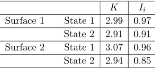
to it (Oy axis). Table 2 shows the values of these indexes for the four plots at our disposal.
One can notice that the kurtosis values for the two seedbeds are close to 3 at ±3% for state 1 and state 2. This sustains the hypothesis of a Gaussian distribution for a seedbed surface. The probability density function (pdf) graph on Figures 1(a) and 1(b) confirms the good agreement between the Gaussian function and the normalised histogram of the heights for the state 1. Similar results are obtained for the state 2.
Table 2. Statistical indexes of studied surfaces.
K Ii
Surface 1 State 1 2.99 0.97 State 2 2.91 0.91 Surface 2 State 1 3.07 0.96 State 2 2.94 0.85
-60 -40 -20 0 20 40 60 0 0.005 0.01 0.015 0.02 0.025 0.03 heights (mm)
probability density function
heights (mm)
-60 -40 -20 0 20 40 60
probability density function 0
0.005 0.01 0.015 0.02 0.025 0.03 (a) (b)
Figure 1. Distribution of heights at state 1 for Gaussian plots. (a) seedbed 1; (b) seedbed 2.
(a) (b)
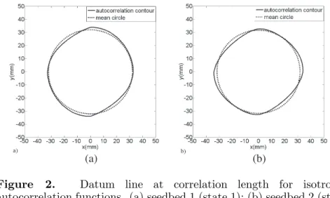
Figure 2. Datum line at correlation length for isotropic autocorrelation functions. (a) seedbed 1 (state 1); (b) seedbed 2 (state 1). The circle is the datum line at average correlation length.
The isotropy index is greater than 95% for the two surfaces at state 1 and autocorrelation contour is very close to circle of average correlation length (see Figure 2). The still high value at state 2 allows keeping the isotropy hypothesis for surface 1. It becomes more questionable for surface 2. However, if our isotropy index is computed with Blaes and Defourny correlation length values for their isotropic surfaces of 60 cm by 60 cm [14], we find at least 83%, which is consistent with our indices.
function is: R (x, y) = s exp − Ã p x2+ y2 l !2r (15)
where s is the rms height, l the correlation length and r, the roughness exponent. The roughness parameters are estimated from experimental autocorrelation C (x, y) by the least squares method. The mean relative error between R (x, y) and C (x, y), which has to be minimized, is: ε = v u u tX i X j µ R(xi, yj) − C(xi, yj) R(0, 0)Lp ¶2 (16) with Lp designing the main lobe length of C (x, y) and the sums being
performed for −Lp/2 ≤ x; y ≤ Lp/2. Table 3 shows the values
estimated along the main lobe of C (x, y), for the two states of the two seedbed surfaces. We can notice that the estimation error given by (16) is weak and smaller than 7%, which illustrates the reliability of estimation. The rms height s and the correlation length l have similar values for surface 1 and surface 2 at state 1. However, the roughness exponent r presents more variability. Comparing state 1 with state 2, s decreases of more than 10% for both surfaces, l shows reverse small variations of ±3% and r presents variations of about 13% also in reverse direction. The decrease of s can be explained by the smoothing of surface during the rainfall event.
In the next section, we study if the changes of these three roughness parameters from state 1 to state 2 are meaningful. Investigations on roughness parameter variability are mainly focused on roughness data obtained by surface-height profiles and have studied
Table 3. Parameters of theoretical autocorrelation function R(x, y).
ε denotes the relative error between R(x, y) and C(x, y) (given by
Eq. (16)). s in mm l in mm r ε Surface 1 state 1 14.9 34.7 0.74 5.2% state 2 12.8 33.3 0.86 7.1% Surface 2 state 1 15.3 34.2 0.89 5.5% state 2 13.7 35.9 0.78 4.6% Average state 1 15.1 34.5 0.80 -Average state 2 13.3 34.6 0.84
-the influence of profile length and number on -the precision of -their estimations. Only few studies have been done on the effect of sampling coverage on statistical roughness parameters (as s and l) using 3D-informations with millimetric resolution [9, 15]. In [14], the bi-dimensional correlation function is computed on squared areas of 60 cm side (that are quite similar in size to the surfaces studied here) and allows the estimation of directional roughness with considerably reduced dispersion.
Then, we study the statistical variability of the roughness parameters due to the single scale Gaussian process and we show from Monte-Carlo simulations that the variation of correlation length l between the two states is not meaningful and falls within the dispersion range observed on the simulated surfaces. A similar conclusion can be established for the roughness exponent r. On the contrary, we show that the change of the rms-height s is relevant.
3.3. Simulation of Surface
The surface realizations are obtained by filtering of Gaussian white noises [17]. The impulse response h(x, y) of the filter is defined as follows:
h(x, y) = F T−1³pF T (R(x, y))
´
(17) where F T designates the Fourier Transform operation and F T−1, the
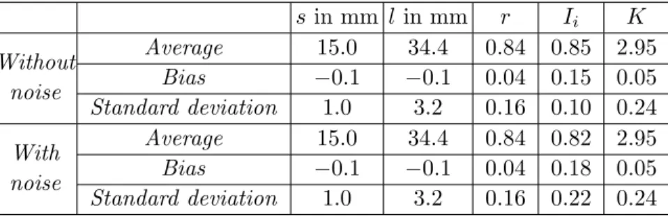
inverse operation. Two simulations of 100 2D-surfaces have been performed in order to test the relevance of roughness parameters s, l, r,
Ii and K obtained in Section 3.2. The surface area is of 2500 cm2 with
a resolution of 1 mm. For the first simulation, the filter was determined with state 1 average values, i.e., s = 15.1 mm, l = 34.5 mm and r = 0.80 as shown in Table 3. The second simulation includes a white noise of 1 mm, modelling possible measurement noise. Table 4 shows that for the first simulation, the average values of s and l estimated over 100 results are obtained with a bias equal to −0.1 mm and the average of r has a bias equal to 0.04, which illustrates the reliability of the simulation process. The estimation of average parameters remains the same in the second case of additional white noise. The additional white noise does not change the values of biases and standard deviations.
The isotropy index is 85% in average (82% in noise condition) and 75% of surfaces have an Iigreater than to 80% (70% in noise condition),
which is satisfactory for an isotropy assumption. Nevertheless, since all the simulated surfaces are supposed to have an isotropic autocorrelation function, the few surfaces with an Ii smaller than 80%
raise a question. Two causes may explain this observation: 1) The isotropic index Ii is computed with estimations of correlation lengths
dependant on the main lobe of autocorrelation function delineation and 2) the estimation of autocorrelation function is altered by the finite dimensions of data. The Kurtosis is 2.95 in average (same in noise condition) and 75% of surfaces have a K within 3±10%, which is satisfactory for a Gaussian assumption. Here again, the remaining 25% of surfaces that are supposed to be Gaussian and depart from a kurtosis of 3, may show some local phenomena that are not compensated by sufficiently great dimensions of data.
We have studied two plots separated from several meters within the same field. Comparing surface 1 with surface 2, the observed differences of rms heights s (from 14.9 mm to 15.3 mm for the state 1 and from 12.8 mm to 13.7 mm for the state 2 as shown in Table 3) are not meaningful with respect to the estimator variance given in the Table 4. Similar conclusions are established for the correlation length and the roughness exponent. Comparing state 2 with state 1, the observed difference of rms height s (from 15.1 mm to 13.3 mm as shown in Table 3) is meaningful. According to Monte-Carlo simulations, s has only 10% of chance to stand below 13.7 mm in the simulation set of state 1. The differences of correlation length and of roughness exponent are not meaningful with respect to the standard deviations defined by Monte-Carlo simulations and given in Table 4. As a conclusion, among the three parameters characterizing the statistical autocorrelation function, the only one that presents a small but meaningful variability between the state 1 and the state 2 is the rms height. Consequently, for the electromagnetic simulations, the correlation length and the roughness exponent are unchanged and we take the values averaged over the two states of surfaces. According to Table 3, l is fixed at 34.55 mm and r at 0.82, respectively. The rms height is fixed at 15.1 mm for state 1 and at 13.3 mm for state 2. Table 4. Results of two-dimensional surface simulations, (a) over 100 surfaces simulated with parameters s = 15.1 mm, l = 34.5 mm and
r = 0.80. (b) Over 100 surfaces simulated with same parameters and
additional white noise.
s in mm l in mm r Ii K Without noise Average 15.0 34.4 0.84 0.85 2.95 Bias −0.1 −0.1 0.04 0.15 0.05 Standard deviation 1.0 3.2 0.16 0.10 0.24 With noise Average 15.0 34.4 0.84 0.82 2.95 Bias −0.1 −0.1 0.04 0.18 0.05 Standard deviation 1.0 3.2 0.16 0.22 0.24
4. ELECTROMAGNETIC SIMULATIONS
In this section, we study the rms height and moisture combined influence upon the direct backscattering coefficients under a given incidence angle and a given frequency. Let us assume that the radar provides a measurement of backscattering coefficient for an agricultural soil in an initial state and for the same soil after a rainfall event. Do these measures allow differentiating the two states of seedbed surfaces? We answer this question and discuss simulation results taking into account the scattering model numerical errors and the radar precision. As an example, we consider electromagnetic configurations in C-band. The incident wavelength is fixed at 5.6 cm, the zenith angle at 40◦ and the azimuth angle at 0◦. Table 5 lists the relative permittivity
values for eight values of the soil moisture Wg in volumetric water
contents (cm3/cm3). The relative permittivity is given by the model
presented in references [18, 19]. The bi-static scattering coefficients are performed over 150 realizations with an area of L × L = 49λ2. The truncation order value is fixed at 21, the spectral resolution at k+/7.
As shown in Table 1, the equivalent spatial resolution ∆xf associated
with these simulation parameters is λ/6, ∆xg is λ/12 and ∆x is λ/18, respectively.
4.1. Surfaces of Electromagnetic Simulations
Edge effects can be present when a finite rough surface is illuminated by a plane wave. Many authors use a tapered-wave incidence in order to reduce the diffracted field at the edge of the surfaces [20, 21]. For the electromagnetic simulations, the local function a(x, y) is defined as the product of b(x, y) by w(x, y). Function b(x, y) is obtained by filtering of a Gaussian white noise (see Section 3.3). Function w(x, y) is a weighing window having continuous first and second derivatives [5– 7, 22]. Function w(x, y) is equal to zero outside the domain |x| , |y| >
L/2 and equal to 1 within the domain −L
2 + lt< x, y < +L2 − lt. The
Table 5. Relative permittivities of soil moistures in volumetric water content (cm3/cm3) at C-band. Moisture Wg (cm3/cm3) 0.05 0.10 0.15 0.20 0.25 0.30 0.35 0.40 Relative permittivity εr= ε0 r− jε00r ε0 r 3.62 4.52 5.94 7.90 10.4 13.9 17.4 20.8 ε00 r 0.19 0.44 0.85 1.42 2.17 3.22 4.30 5.30
length lt defines a transition zone where w(x, y) changes continuously from 1 to 0. For the numerical simulations, lt is fixed at λ/2. As shown in [6, 7], the use of this weighing function is effective and one can find results obtained in the literature by other methods associated with tapered-wave incidence.
4.2. Analysis of Numerical Errors
Because the length L and number of realizations Nr have finite
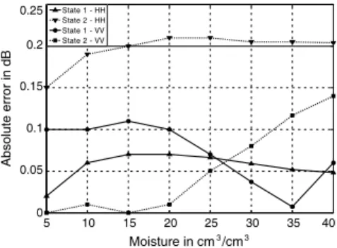
values and as the spatial resolution does not tend to zero, the results present numerical errors [8]. For the different values of rms height and permittivity, we quantify the errors on backscattering coefficients obtained with the simulation parameters listed in the first line of Table 1. For this purpose, we define a reference configuration for which we assume that accuracy on the results is ideal. The simulation parameters of this reference configuration are given in the second line of Table 1. Because computing time is too high for large 2D-surface realizations, we determine the errors on the results from electromagnetic 2D-simulations applied to 1D-surface realizations [5] and we assume that the errors does not change for electromagnetic 3D-simulations applied to 2D-surface realizations. Figure 3 shows the absolute errors between the backscattering coefficients associated with the two series of parameters for both surface states and polarizations. This estimated error takes into account three effects: a) the effects due to the finite value of surface area, b) the statistical error due to the finite value of number of realizations, c) the effects due to the finite value of spatial resolution. Errors are smaller than 0.21 dB. For the surfaces under consideration, we can retain the simulation parameters given in the first line of Table 1 for analyzing the backscattering signal.
5 10 15 20 25 30 35 40 0 0.05 0.1 0.15 0.2 0.25 Moisture in cm /cm3 3 Absolute error in dB State 1 - HH State 2 - HH State 1 - VV State 2 - VV
Figure 3. Absolute errors on numerical results versus the moisture content. Simulation parameters are given in Table 1.
The typical resolution cell of SAR systems is higher than the surface area considered in this paper. What should be kept in mind is that the scattering signal does not depend on the surface size as long as the surface area is large enough to contain many correlation lengths and many wavelengths. The backscattering coefficients are performed over 150 realizations with an area of L × L = 49λ2. The length L is equal to 7 wavelengths and contains more than 11 correlation
lengths. The backscattering coefficient varies very little for lengths greater than 7 wavelengths as shown in Figure 3. Consequently, our numerical results can be considered as good predictions of signals measured by radar having a higher resolution cell. Nevertheless, such an approach assumes that the soil under study is a stationary spatial process and that the statistical properties do not change from one cell to another. Moreover, this assumes that the ground is flat or that their low-frequency components can be overlooked.
4.3. Influence of the Radar Precision
Figure 4 shows the backscattering coefficient as a function of soil moisture for HH-polarization. Figure 5 shows results for V V -polarization. For the surface under consideration, the rain has a dual effect on the agricultural area. First, the rainfall events tend to flatten the soils and after a rainfall, the roughness decreases. Second, under the effect of rain, the moisture increases. On the electromagnetic point
5 10 15 20 25 30 35 40 -20 -19 -18 -17 -16 -15 -14 -13 -12 -11 -10 Backscattering coefficient in dB Polarization HH State 1 State 2 Moisture in cm /cm3 3 Figure 4. HH-polarized
backscattering coefficients versus the moisture content. Symbols indicate results obtained by Monte-Carlo simulations. Curves indicate results obtained by (18).
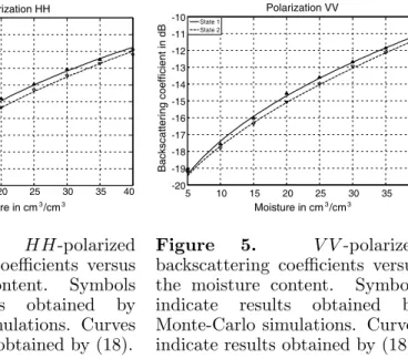
State 1 State 2 Backscattering coefficient in dB -20 -19 -18 -17 -16 -15 -14 -13 -12 -11 -10 5 10 15 20 25 30 35 40 Moisture in cm /cm3 3 Polarization VV Figure 5. V V -polarized
backscattering coefficients versus the moisture content. Symbols indicate results obtained by Monte-Carlo simulations. Curves indicate results obtained by (18).
of view, these two effects are opposite. As shown in Figures 4 and 5, the backscattering coefficient decreases with the roughness and increases with the moisture. Nevertheless, the average difference between the backscattering coefficients corresponding with both roughness states is equal to 0.3 dB for both polarizations. Such a difference is not meaningful compared to the numerical error (0.21 dB) due to finite values of simulations parameters. For the studied configuration, the moisture content is the discriminating parameter for the backscattering coefficient in C-band.
The backscattering coefficient can be modelled as a function of the moisture by:
[σ0]dB = a + bWgc (18)
For each polarization, the values of the three parameters a, b and c are listed in Table 6. Figures 4 and 5 show the curves obtained from this relationship. Comparisons are good. For the configurations under study, this relationship allows analyzing results with respect to the radar precision.
Let us assume that the exact values [σ01]dB and [σ02]dB of the
backscattering coefficient for the two states of soil are given by Equation (18). For a precision ∆σdB, the measured backscattering coefficients [σm1]dB and [σm2]dB are included in the following ranges:
[σ01]dB− ∆σdB ≤ [σm1]dB ≤ [σ01]dB+ ∆σdB
[σ02]dB− ∆σdB ≤ [σm2]dB ≤ [σ02]dB+ ∆σdB (19)
where [σ02]dB> [σ01]dBbecause under rain effect, the moisture content
increases. Moreover, let us assume an upper limit of moisture content of 0.45 cm3/cm3. The differences between the measured backscattering
coefficients are meaningful if one of the following conditions is satisfied: [σ01]dB+ ∆σdB ≤ [σ02]dB− ∆σdB (20a)
[σ02]dB+ ∆σdB ≤ [σ01]dB− ∆σdB (20b)
The condition (20a) occurs when the effect of moisture increasing due to the rain is more important than roughness decreasing effect. The Table 6. Parameters of relationship (18) giving the backscattering coefficient as a function of the moisture content.
Polarization State of surface a b c
HH 1 −27.05 4.38 0.34
2 −23.68 1.90 0.49
V V 1 −24.95 2.74 0.44
condition (20b) represents the opposite case. Substituting (18) into (20a) and (20b), we find:
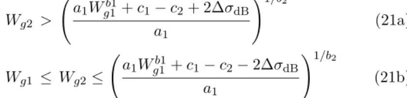
Wg2 > Ã a1Wg1b1+ c1− c2+ 2∆σdB a1 !1/b2 (21a) Wg1 ≤ Wg2≤ Ã a1Wg1b1+ c1− c2− 2∆σdB a1 !1/b2 (21b) where Wg1 and Wg2are the moisture contents associated with the two roughness states. For a given value of moisture Wg1, the differences between the measured backscattering coefficients are meaningful only if the moisture Wg2 checks one of these two conditions (21a) or (21b).
5 10 15 20 25 30 35 40 5 10 15 20 25 30 35 40 45 ∆σ = 0.25 dB - HH W g1 W g2 5 10 15 20 25 30 35 40 5 10 15 20 25 30 35 40 45 ∆σ = 0.50 dB - HH W g1 W g2 5 10 15 20 25 30 35 40 5 10 15 20 25 30 35 40 45 ∆σ = 0.75 dB - HH W g1 W g2 5 10 15 20 25 30 35 40 5 10 15 20 25 30 35 40 45 ∆σ = 1 dB - HH W g1 W g2
Figure 6. Final moisture content versus initial moisture content (in cm3/cm3) under HH polarization. The white area is defined by
the condition (21a). Inside the gray area, the measurements of the backscattered signal do not permit to differentiate the two states of the agricultural soil.
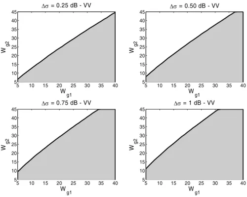
5 10 15 20 25 30 35 40 5 10 15 20 25 30 35 40 45 ∆σ = 0.25 dB - VV W g1 W g2 5 10 15 20 25 30 35 40 5 10 15 20 25 30 35 40 45 ∆σ = 0.50 dB - VV W g1 W g2 5 10 15 20 25 30 35 40 5 10 15 20 25 30 35 40 45 ∆σ = 0.75 dB - VV W g1 W g2 5 10 15 20 25 30 35 40 5 10 15 20 25 30 35 40 45 ∆σ = 1 dB - VV W g1 W g2
Figure 7. Final moisture content versus initial moisture content (in cm3/cm3). Same as Figure 6 but under V V polarization.
Figure 6 shows the areas defined from (21) for four values of the precision ∆σdB (0.25, 0.5, 0.75 and 1 dB) under HH-polarization.
Figure 7 shows results under V V -polarization. The white area is defined by the condition (21a). For the configuration under study, the first condition (21a) is more restrictive than the second one (21b). If Wg1 and Wg2 are in a gray area, the conditions are not checked and the measurements of the backscattered signal do not discriminate between the two states of surfaces. Figures 6 and 7 clearly show that the ability of the measurement system to differentiate seedbed surfaces is linked to its precision. Conditions are all the more restrictive than the value of ∆σdB increases. The condition (21a) on the final moisture
Wg2 is all the more restrictive than the initial moisture Wg1 is high.
For the configurations under study, the condition is less restrictive for the V V -polarization.
5. CONCLUSION
First, we implemented a consistent roughness parameterisation relying on bidimensional surface measurement. We considered initial plots of seedbed surfaces just after tillage. Each initial plot was submitted to a 40 mm hr−1 simulated rainfall during 30 minutes. Soil surface
DEMs measuring 50 cm by 50 cm with a fine resolution of about 1 mm in horizontal and vertical directions were used. We showed that these seedbed surfaces can be modelled as isotropic Gaussian processes. We showed that the autocorrelation function is well characterized by three parameters: the rms height, the correlation length and the roughness exponent. These parameters were estimated from the experimental bidimensional autocorrelation function. We showed that the height variation induced by the rainfall smoothing is meaningful in contrast to variations of the correlation length and the roughness exponent.
Second, we studied the roughness and moisture influence upon the direct backscattering coefficients and we discussed results taking into account the numerical errors and the precision of radar. For electromagnetic simulations, in agreement with the characterization of soils, we considered that the rms height is the only roughness parameter that changes after the rainfall event. The backscattering coefficient was estimated by averaging the scattering amplitudes over several realizations. For each realization, the scattering amplitudes were obtained by the C-method. We defined a procedure in order to quantify numerical errors on the backscattering coefficients. Errors are smaller than 0.21 dB. Nevertheless, the difference between the backscattering coefficients associated with the two soil states is equal to 0.3 dB for both polarizations. Such a difference is not meaningful compared to the numerical error. As a result, for the configuration analyzed with the C-method, the moisture content is the discriminating parameter for the backscattering coefficient in C-band. For a given radar precision, we defined the conditions that must be checked by the moisture contents so that the measurements of backscattering coefficients can differentiate the seedbed surface in the initial state just after tillage and in the second state after the rainfall event. Besides the moisture content conditions, we showed that the ability of the sensor to discriminate the state of surfaces is clearly linked to its precision.
In this paper, the roughness measurements are limited to some plots of seedbed soils. Moreover, the soil is a loamy typic hapludalf with moderate roughness and unmarked tillage patterns. As a result, they can hardly be considered representative of agricultural surface roughness changes due to rain events. Nevertheless, the approach adopted in this paper to discuss the relevance of the values of roughness
parameters is efficient because it allows defining the estimator bias and its variance. This approach can be extended for others soil types. Our middle-term objective is the construction of a database by means of roughness and moisture content measurements, radar signatures and electromagnetic simulations associated with different soil types and different soil textural compositions [23, 24]. We wish to establish from this database relationships giving the backscattering coefficients as functions of incidence parameters (incidence angle, frequency) and soil parameters. Such relationships used for multifrequency or angle configurations will be useful for retrieving soil moisture and surface roughness with consideration of sensor precision [25–28].
REFERENCES
1. Chandezon, J., D. Maystre, and G. Raoult, “A new theoretical method for diffraction gratings and its numerical application,” J.
Optics (Paris), Vol. 11, No. 4, 235–241, 1980.
2. Li, L. and J. Chandezon, “Improvement of the coordinate transformation method for surface-relief gratings with sharp edges,” J. Opt. Soc. Am. A, Vol. 13, No. 11, 2247–2255, 1996. 3. Granet, G., “Analysis of diffraction by surface-relief crossed
gratings with use of the Chandezon method: Application to multilayer crossed gratings,” J. Opt. Soc. Am. A, Vol. 15, No. 5, 1121–1131, 1998.
4. Duss´eaux, R. and C. Baudier, “Scattering of a plane wave by 1-dimensional dielectric rough surfaces — Study of the field in a nonorthogonal coordinate system,” Progress In Electromagnetics
Research, Vol. 37, 289–317, 2002.
5. Baudier, C., R. Duss´eaux, K. S. Edee, and G. Granet, “Scattering of a plane wave by one-dimensional dielectric random surfaces — Study with the curvilinear coordinate method,” Waves Random
Media, Vol. 14, No. 1, 61–74, 2004.
6. A¨ıt Braham, K., R. Duss´eaux, and G. Granet, “Scattering of electromagnetic waves from two-dimensional perfectly conducting random rough surfaces — Study with the curvilinear coordinate method,” Waves Random Complex Media, Vol. 18, No. 2, 255–274, 2008.
7. Duss´eaux, R., K. A¨ıt Braham, and G. Granet, “Implementation and validation of the curvilinear coordinate method for the scat-tering of electromagnetic waves from two-dimensional dielectric random rough surfaces,” Waves Random Complex Media, Vol. 18, No. 4, 551–570, 2008.
8. Marchand, R. T. and G. S. Brown, “On the use of finite surfaces in the numerical prediction of rough surface scattering,” IEEE
Trans. Antennas and Prop., Vol. 47, No. 4, 600–604, 1999.
9. Taconet, O. and V. Ciarletti, “Estimating soil roughness indices on a ridge-and-furrow surface using stereo photogrammetry, ” Soil
and Tillage Research, Vol. 93, No. 1, 64–76, 2007.
10. Fung, A. K., Z. Li, and K. S. Chen, “Backscattering from a randomly rough dielectric surface,” IEEE Trans. Geosci. Remote
Sens., Vol. 30, No. 3, 356–369, 1992.
11. Franceschetti, G. and D. Riccio, Scattering, Natural Surfaces and
Fractals, Elsevier, 2007.
12. Voronovich, G., Wave Scattering from Rough Surfaces, Springer, Berlin, 1994.
13. Taconet, O., E. Vannier, and S. Le H´egarat-Mascle, “A contour-based approach for clods identification and characterization on a soil surface,” Soil and Tillage Research, Vol. 109, No. 2, 123–132, 2010.
14. Blaes, X. and P. Defourny, “Characterizing bidimensional roughness of agricultural soil surfaces for SAR modelling,” IEEE
Trans. Geosci. Remote Sensing, Vol. 46, No. 12, 4050–4061, 2008.
15. Marzahn, P. and R. Ludwig, “On the derivation of soil surface roughness from multi parametric PolSAR data and its potential for hydrological modelling,” Hydrology Earth System Sciences, Vol. 13, No. 6, 381–394, 2009.
16. Wu, S. C., M. F. Chen, and A. K. Fung, “Scattering from non-Gaussian randomly rough surfaces — Cylindrical case,” IEEE
Trans. Geosci. Remote Sensing, Vol. 26, No. 6, 790–798, 1988.
17. Fung, A. K. and M. F. Chen, “Numerical simulation of scattering from simple and composite surface,” J. Opt. Soc. Am. A, Vol. 2, No. 12, 2274–2283, 1985.
18. Wang, J. R. and T. J. Schmugge, “An empirical model for the complex dielectric permittivity of soils as a function of water content,” IEEE Trans. Geosci. Remote Sensing, Vol. 18, No. 4, 288–295, 1980.
19. Tsang, L., J. A. Kong, K. H. Ding, and C. O. Ao, Scattering
of Electromagnetic Waves — Numerical Simulations,
Wiley-Interscience, New-York, 2001.
20. Thorsos, E. I., “The validity of the Kirchhoff approximation for rough surface scattering using a Gaussian roughness spectrum,”
21. Johnson, J. T., “Surface currents induced on a dielectric half-space by a Gaussian beam: An extended validation for point matching method of moment codes,” Radio Sci., Vol. 32, No. 3, 923–934, 1997.
22. Spiga, P., G. Soriano, and M. Saillard, “Scattering of electromagnetic waves from rough surfaces: A boundary integral method for low-grazing angles,” IEEE Trans. Antennas and Prop., Vol. 56, No. 7, 2043–2050, 2008.
23. Li, J., L.-X. Guo, and H. Zeng, “FDTD method investigation on the polarimetric scattering from 2-D rough surface,” Progress In
Electromagnetics Research, Vol. 101, 173–188, 2010.
24. Guo, L.-X., Y. Liang, J. Li, and Z.-S. Wu, “A high order integral SPM for the conducting rough surface scattering with the tapered wave incidence-TE case,” Progress In Electromagnetics Research, Vol. 114, 333–352, 2011.
25. Zribi, M. and M. Dechambre, “A new emperical model to retrieve soil moisture and roughness from C-band radar data,” Remote
Sensing Env., Vol. 84, 42–52, 2002.
26. Singh, D. and A. Kathpalia, “An efficient modeling with GA approach to retrieve soil texture moisture and roughness from ERS-2 SAR data,” Progress In Electromagnetics Research, Vol. 77, 121–136, 2007.
27. Mittal, G. and D. Singh, “Critical analysis of microwave scattering response on roughness parameter and moisture content for periodic rough surfaces and its retrieval,” Progress In
Electromagnetics Research, Vol. 100, 129–152, 2010.
28. Prakash, R., D. Singh, and N. P. Pathak, “The effect of soil texture in soil moisture retrieval for specular scattering at C-band,” Progress In Electromagnetics Research, Vol. 108, 177–204, 2010.