HAL Id: hal-02090686
https://hal.archives-ouvertes.fr/hal-02090686
Submitted on 23 Apr 2019HAL is a multi-disciplinary open access archive for the deposit and dissemination of sci-entific research documents, whether they are pub-lished or not. The documents may come from teaching and research institutions in France or abroad, or from public or private research centers.
L’archive ouverte pluridisciplinaire HAL, est destinée au dépôt et à la diffusion de documents scientifiques de niveau recherche, publiés ou non, émanant des établissements d’enseignement et de recherche français ou étrangers, des laboratoires publics ou privés.
Spectral mapping method based on intervals of
comonotonicity for modelling of radiative transfer in
non-uniform gaseous media
Frédéric André, Vladimir Solovjov, Brent Webb, Mathieu Galtier, Philippe
Dubuisson
To cite this version:
Frédéric André, Vladimir Solovjov, Brent Webb, Mathieu Galtier, Philippe Dubuisson. Spectral mapping method based on intervals of comonotonicity for modelling of radiative transfer in non-uniform gaseous media. Journal of Quantitative Spectroscopy and Radiative Transfer, Elsevier, 2019, 229, pp.33-39. �10.1016/j.jqsrt.2019.02.030�. �hal-02090686�
SPECTRAL MAPPING METHOD BASED ON
INTERVALS OF COMONOTONICITY FOR
MODELLING OF RADIATIVE TRANSFER IN
NON-UNIFORM GASEOUS MEDIA
Frédéric ANDRE*,1, Vladimir P. SOLOVJOV2, Brent W. WEBB2, Mathieu GALTIER1,
Philippe DUBUISSON3
1 Univ Lyon, CNRS, INSA-Lyon, Université Claude Bernard Lyon 1, CETHIL UMR5008, F-69621 Villeurbanne, France
2 Brigham Young University, 350G EB, Provo, UT 84602 USA
3 Laboratoire d’Optique Atmosphérique, Univ. Lille – 5900 Lille, France
ABSTRACT. The aim of this work is to describe a Spectral Mapping Method (SMM) to split
spectral intervals into smaller sets of wavenumbers, called intervals of comonotonicity, over
which gas spectra in distinct states are rigorously linked through a strictly increasing function.
Over small intervals of comonotonicity, the proposed method becomes, in theory, exact. The
step-by-step process of construction of intervals of comonotonicity is described and explained.
The present work focuses on the two-cell problem. Despite its full generality for the treatment
of the blurring effect in k-distribution approaches, the strength of the method is illustrated: 1/
with a high number of subintervals on an IR signature configuration, widely recognized as
among the most challenging in band model theory; 2/ with only two subintervals, in a highly
non-uniform two-cell configuration. Comparisons with reference Line-By-Line calculations
and a mapping technique founded on a scaled map illustrate its relevance for radiative heat
transfer and spectroscopic applications.
KEYWORDS: gas radiation, non-uniform, spectral mapping method (SMM), intervals of
NOMENCLATURE
g cumulative k-distribution – Eq. (1) k absorption coefficient (cm-1)
u abscissa at the origin for the lines used to split the g-g plot (Sections 2 and 3)
u scaling coefficient (Section 4)
Greek symbols
spectral band width (cm-1)
spectral absorption coefficient (cm-1)
spectral mapping function (cm-1)
wavenumber (cm-1)Subscripts / superscript
1. INTRODUCTION
Extension of approximate models of gas radiation from uniform to non-uniform paths is among
the most difficult problems in gas radiation modeling [1]. Although many methods are accurate
enough for radiative heat transfer applications, most of them do not permit to achieve a
precision sufficient for narrow and wide band spectroscopic (environmental, etc.) applications.
In these cases, advanced techniques to improve approximate models of gas radiation for general
non-uniform applications are required. These techniques can be organized in two main
categories: Multiple-Line-Group methods [1] and Spectral Mapping techniques.
Multiple-Line-Group (MLG) approaches are among the oldest techniques. They first appeared in 1962 as part of Wyatt’s quasi-random band model [2], and consist of an explicit grouping of spectral lines according to values of their linestrengths. The idea of combining spectral lines
with similar lower state energy levels appeared in the 70s, as a way to ameliorate the treatment
of highly non-isothermal paths. Early methods based on this idea are described in Refs. [3-6].
Recent appellations for these approaches are the fictitious gases [7] and the multi-scale method
described in Baradwaj and Modest [8]. The method presented in Ref. [8] mostly reformulates
in different words the approach proposed a few years earlier in Ref. [9]. The output of a MLG
treatment is a set of groups of spectral lines whose centers are assumed to be statistically
independent, from one group to another.
Spectral Mapping Methods (SMM) seek to avoid the use of simplifying assumptions to treat
non-uniform gaseous paths (constant absorption coefficient, scaling, etc.) by iteratively splitting the spectral interval associated with the model’s definition into sub-intervals over which these non-uniform treatments are not assumptions but actual properties of gas spectra. The output of
a SMM treatment is a set of spectral intervals over which a particular relationship between high
resolution spectra in distinct states (scaling, correlation / comonotonicity, etc.) can be assumed
non-uniformities. Application of SMM requires high resolution spectral data, which explains why
these techniques are more recent than MLG. The first SMM was in fact proposed by West and
Crisp in 1990 [10]. It consists in building sub-intervals, or bins, in such a way that gas spectra
are constant over the bins at each spatial location along non-uniform paths. This technique was
improved recently in Refs. [11,12]. Other methods produce intervals over which gas spectra
can be treated as scaled. Modest and co-workers’ multi-group (MG) [13] (not to be confused with Ludwig’s [3] or Khodyko / Vitkin [4-6] multi-group methods which are both founded on MLG) and multi-spectral techniques [14-17] fall in this category and differ principally by the
way the spectral intervals are built. In two recent papers [18,19], efforts were made by Hu and
Wang to improve the grouping scheme used in the Multi-Scale Multi-Group (MSMG) method
of Modest by attempting to replace constraints on scaling coefficients, as used in the original
version, by pragmatic criteria based on a correlated view. The necessity to treat differently
single species and mixtures is closely related to the initial choice made by the authors to apply
the MSMG method for their problem.
When formulated and applied properly, both MLG and SMM have the potential to improve
significantly the treatment of path non-uniformities. No combinations of the two techniques,
which are by construction redundant, are in this case required.
This work proposes a SMM technique that allows the building of spectral intervals over which
gas spectra in distinct states are rigorously linked through a strictly increasing function.
Accordingly, over these intervals that will be from now on referred to as intervals of
comonotonicity, the two spectra at the distinct states can be related through monotonically
increasing functions: spectra are called comonotonic [20], and the Ck / CKD approaches are
exact. Notice that Ck and CKD acronyms represent the same method (the so-called Correlated
mostly encountered in Mechanical Engineering (Ck) whereas the other one is more usual in
Atmospheric Sciences (CKD).
The present method improves k-distribution methods by directly addressing the blurring effect
of non-uniform k-distribution approximations: this effect is encountered both for high
temperature (as considered here for illustration) and atmospheric applications. The
simplification of the treatment of path non-uniformities that is provided by the present SMM
results from the construction of spectral intervals over which this blurring effect can be
effectively eliminated. The step-by-step process to construct intervals of rigorous
comonotonicity, and thus “correlation” or “zero-blurring”, is described. It is applied here to
narrow spectral intervals but its extension to any band width is possible since it only requires
the specification of the cumulative k-distributions of the gas in distinct states: any particularity
of the problem under study (width of the band, possible influence of optical filters and / or
non-constant blackbody function) is already included in the calculation of the cumulative
k-distribution. Application of the method to highly non-uniform situations, one of which is
representative of the classically challenging IR plume signature calculation, illustrates the
relevance of the method. The present grouping scheme can be used alone, as proposed here, or
together with other techniques for which it can provide a relevant initial guess at the earliest
stage of their iterative process.
2. BUILDING INTERVALS OF COMONOTONICITY
Let us consider two gas spectra at two distinct thermophysical states for which the spectral
absorption coefficients in the two states are 1 and 2, respectively. The cumulative k-distribution functions that correspond to these two spectra are:
1
1 2 i i i i g k H k d , i ,
(1)where H is the Heaviside step function. The problem is formulated here within the frame of
narrow band approaches but can be extended to any other band, up to the full spectrum, by
replacing d in Eq. (1) by any weighting function of the form
d where
0 and
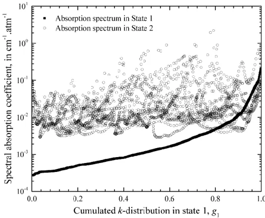
d 1.We start our analysis by plotting the absorption spectra for the two thermophysical states not
as functions of wavenumbers, as in usual LBL representations, but with respect to the
cumulative distribution function of the absorption coefficient in State 1,
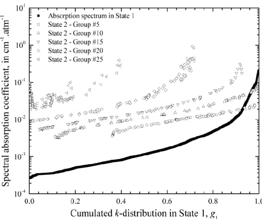
1 1g . State 1 is a 1 % H2O – 99 % N2 mixture at 300 K ; State 2 is 10 % H2O – 90 % N2 at 1500 K. The 25 cm-1 narrow band considered for the following figures is centered at 3400 cm-1, in the 2.7 µm band of H2O. This spectral region is widely used in IR plume signature studies [9,21].
For this purpose, we start with the high resolution (10-2 cm-1) spectra in the two states, provided
as vectors
1 2 1 1 1 , ,.., N and
1 2 2 2 2 , ,.., N where
1, 2,.., is the set of N
wavenumbers used in the LBL calculation, and calculate two new vectors
1 2
1 1 1 1 , 1 ,.., 1 N g g g and
1 2 2 2 2 2 , 2 ,.., 2 N g g g by application of Eq. (1). If one sets
1 2 1 1 1 1 , 1 ,.., 1 Ng g g as abscissa axis and plots
1 2 1 1 1 , ,.., N and
1 2
2 2 2 , ,.., N with respect to this vector, one receives Figure 1. After the change of abscissa axis from wavenumbers to
11
g , the gas spectrum in State 1 is monotonically increasing (this is the main principle of the k-distribution method) whereas the
absorption spectrum in State 2 is not (in the present case but this observation is rather general)
an increasing function of
1 1g . This departure from monotonicity is the main source of error
Our aim is to build spectral intervals over which gas spectra are comonotonic viz. to extract
subsets of points from the cloud of circles (absorption coefficient in State 2 reorganized with
respect to
1 1g - in other words, values of 2 at the wavenumbers where 1 is associated with the pseudo-spectral wavenumber
11
g ) of Figure 1 that increase with respect to g1.
Figure 1. Example of two spectra reordered with respect to the same (related to State 1)
cumulative k-distribution function. Gas spectra are clearly not comonotonic / correlated.
For this purpose, we will mostly follow the same steps as in Ref. [15] where the objective was
to construct sub-intervals over which gas spectra are scaled. However, the starting point is
slightly different. Indeed, the main difference between the two approaches (scaled in [15] or
correlated / comonotonic here) is that we will replace the C-curves of Ref. [15] (2-dimensional
parametric curve 1 2
1 2
plot of
1
21 1 2 2
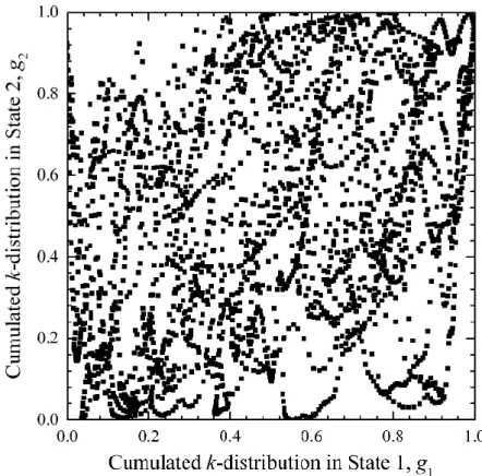
g g , g g in the (g1, g2)-plane). This kind of representation is not new in the radiative heat transfer literature and can be found for instance in Ref. [22] to illustrate the
blurring effect of k-distribution methods viz. to show their possible departure from the so-called “correlated” assumption. An example of g-g plot is given in Figure 2 corresponding to the same set of LBL data as for Figure 1. This figure was obtained by setting
1 2
1 1 1
1 , 1 ,.., 1 N
g g g as abscissa axis and plotting
1 2 2 2 2 2 , 2 ,.., 2 N g g g with respect to
1 1 1g g . For the sake of legibility, only the points associated with the
discrete wavenumbers used in the LBL calculation of 1 2
and
are depicted.
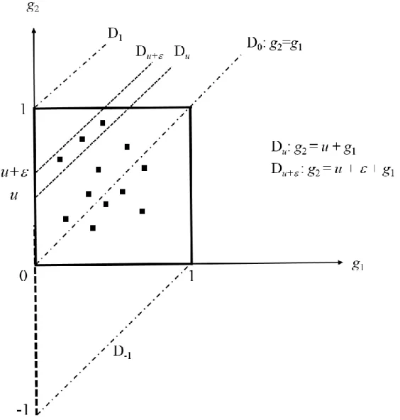
Figure 3 represents a simplified model of g-g plot. If gas spectra were actually “correlated”,
their cumulative distribution would take equal values at all wavenumbers and all the points
1
21 1 2 2
g g , g g would be aligned on the straight diagonal line D0. As gas spectra are not correlated / comonotonic in the case considered, points of coordinates
1
21 1 2 2
g g , g g can be found in various regions of the unit square. The building of
sub-intervals of comonotonicity consists in splitting the unit square in a pertinent way so as to define
these intervals. In other words, we seek to identify using Fig. 2 wavenumber intervals where
the two spectra are related through a strictly increasing function, viz. over which they share the
same monotonicity by increasing or decreasing simultaneously.
Let us focus our attention on the set of wavenumbers
u built by grouping together the points located between the two lines Du and Du+, where is a positive increment and u takes values between -1 and 1. At all these spectral locations, one has:
2 12 1
ug g u (2)
Consequently, for small increments , all the values of the absorption coefficient in State 2 over
u
are associated with values of the absorption coefficient in State 1 through the following linear relationship:
2
1
2 1 , g u g u (3) or equivalently:
2 1 1 1 1 2 1 u , where u 2 1 g u g k g u g k (4)Eq. (4) shows that the two absorption spectra 1 and 2 are linked to each other through a strictly increasing function , that depends on u, at all spectral locations u
u .In this case, the cumulative-k distributions restricted to the interval
u which are defined for the two states 1 and 2 as:
1 , 1, 2 i i i i u g k u H k d i u
(5)take equal values for any wavenumber inside
u and follow rigorously:
1 2
1 2 ,
g u g u u (6) This relationship arises directly from the equalities Eqs. (3,4) and the definition of
other through a strictly increasing function in which case their rank / cumulative distribution
functions are equal [20]. Intervals
u thus correspond to intervals of comonotonicity, i.e., spectral intervals over which gas spectra are comonotonic.Based on the same principle, the unit square can be discretized into diagonal belts at fixed
values of u. All the points that belong simultaneously to the g-g plot and a given belt can then
be grouped to define a spectral interval over which gas spectra are comonotonic and,
consequently, over which the Ck / CKD method is exact. By varying the parameter u between
-1 and 1 one reconstructs the unit square and thus the set of wavenumbers (the narrow band
considered in this work) .
3. APPLICATION
The results provided in this section are based on the same LBL dataset as described in Ref. [15].
They use spectral line parameters taken from HITEMP2010 [23] as inputs. The two states
considered in this section are the same as for the previous figures: State 1 is a 1 % H2O – 99 % N2 mixture at 300 K ; State 2 is 10 % H2O – 90 % N2 at 1500 K. As noticed earlier, spectra were restricted to the 25 cm-1 spectral band centered at 3400 cm-1 for Figures 1,2,4,5.
Building intervals of comonotonicity from the sets of vectors described in the previous section
up to radiative heat transfer calculations requires several steps:
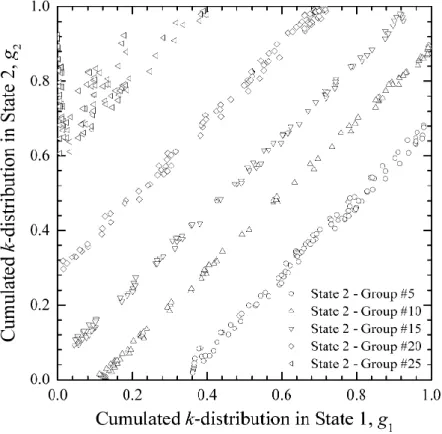
A / the first step consists of splitting the g-g plot of Figure 2 into different diagonal belts, each
of which corresponds to a distinct value of the parameter u. The splitting process was done by:
1/ evaluating the distribution function F of the spectral variable
2 12 1
g g ; 2/ dividing the unit interval [0,1] into N + 1 equally spaced values Xi, i1,N1; X10; XN1 ; 3/ 1 solving F u
i Xi to define bounds ui, i1,N for the variable u; 4/ the i-th belt then 1 consists of all wavenumbers for which
2 12 1 1
i i
In this section, N = 25 belts were constructed by this method. Each belt contains roughly the
same number of points (100 ± 2 spectral values of the absorption coefficients). Results (only a
few subsets are plotted for legibility) are depicted in Figure 4.
Figure 4. Discretization of the g-g plot into diagonal belts
B/ Next, all the points inside a diagonal belt, made of many noncontiguous intervals, are
prescribed to the same group. This defines an ensemble of N = 25 groups together with their
corresponding intervals
u , u
1,1
. An inverse transformation 1 2g is then applied to
all the elements in each group and the corresponding absorption coefficients are plotted with
the same symbols as in the g-g plot of Figure 4. This yields Figure 5. The simple process
Figure 1 subsets of k-values that almost share the same monotonicity with respect to g1 in the two states.
Figure 5. Subsets of comonotonic absorption coefficients (groups)
C/ In the final step, each set of absorption coefficients in a group of wavenumber
u is treated as an independent spectrum over which a k-distribution parameterization is applied viz.a distribution function is evaluated over the set of k-values inside a belt
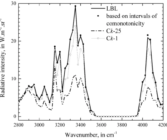
u and then inverted to provide an ensemble of corresponding gray gas absorption coefficients. Outcomesof this method are plotted in Figures 6 and 7. These figures correspond to a plume signature
situation. For the narrow band averaged IR plume signature calculation of Figure 6, the length
of the cold (State 1) path is 1000 m and that of the hot path (State 2) is 80 cm. Gases are at
atmospheric pressure. Figure 6 shows the predicted radiative intensity exiting the cold layer and
reference LBL calculations. For comparison purposes, results of a Ck-1 model (Ck / CKD model
built on 1 cm-1 wide spectral intervals) averaged over 25 cm-1 are also provided together with a Ck-25 model (Ck / CKD model built on 25 cm-1 wide spectral intervals). The two approaches (Ck-1 and the Ck model based on intervals of comonotonicity) use weights and nodes based on
a 7th order Gauss-Legendre quadrature and thus share the same computational cost after the belts of comonotonicity are determined. The Ck-25 model uses the same type of quadrature at
order 25. The approximation based on the intervals of comonotonicity clearly outperforms that
obtained with a discretization of the 25 cm-1 narrow bands into contiguous spectral intervals, viz. Ck-1.
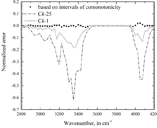
Figure 7. same as Figure 6 but expressed as the normalized error defined as the difference
Model intensity – LBL intensity divided by the maximum intensity over the spectral range
4. COMPARISON WITH A MAPPING TECHNIQUE BASED ON INTERVALS OF SCALING
As emphasized in the introduction, there exist many mapping methods in the literature to
improve approximate models of gas radiation in non-uniform situations. Among them,
techniques based on intervals of scaling are probably the simplest. They are all built on the
same simple idea, explained below.
At high spectral resolution, gas spectra are rigorously scaled. However, the scaling property
cannot, in general, be extended to spectral bands since, for any two absorption spectra 1 and
2
of the same molecule in distinct states, the ratio u 2 1 is rarely a constant over a contiguous set of wavenumbers of non-null width . One can however define, as for 1 and
2
, a distribution function for this new spectral variable u 2 1 :
1
F u H u u d u u
P (7)This distribution function can be used to define intervals of scaling. Indeed, they can be built
by application of the following steps: 1/ the unit interval [0,1] is divided into N + 1 equally
spaced values Xi, i1,N1; X10; XN1 ; 2/ 1 F u
i Xi is solved, where F is nowgiven by Eq. (7) and represents the distribution function of scaling coefficients, which provides
bounds ui, i1,N for the variable 1 u 2 1 ; 3/ subintervals are then obtained by grouping together all wavenumbers for which
2 1 1 i i u u
; 4/ over these intervals, the ratio
2 1
u is roughly a constant (in the same way that when applied directly to gas spectra the method provides gray gases). Absorption spectra can thus be treated as scaled (their ratio is a
It can be noticed that for large N, a constant value of the ratio of the two spectra is a fair
approximation inside each of the subintervals provided by this method so that a mean scaling
coefficient can be realistically introduced. For small values of N, however, the use of the Ck /
CKD method can correct errors due to non-constant scaling coefficients and should be
preferred, as suggested in Ref. [13]. This is the method selected in this section since the choice
N=2 was made. Indeed, since the two methods that we want to compare (based on intervals of
scaling or comonotonicity) converge toward the exact solution at infinite values of N, their
comparison only has relevance for small values of N. Notice also that the two methods based
on intervals of scaling and comonotonicity share in this case almost the same RTE solver. Only
the intervals used to construct conditional (viz. restricted to subintervals, as introduced in Eq.
(5) for the comonotonic case) k-distribution functions differ.
This method to construct intervals of scaling is not exactly the same as used, for instance, by
Zhang and Modest in the multi-group method [13] or in Refs. [14-17] for the multispectral
approach, both of which use some criterion on spectral scaling coefficients over sequences of
thermophysical states to construct intervals of scaling. Here, only two states are treated.
However, these techniques are founded on the same principle (aggregate intervals in such a way
that the ratio of any two spectra is a constant) and should provide, in theory, exactly the same
results as those provided by the present method.
The two spectral mapping techniques (scaling / comonotonicity intervals) are compared and
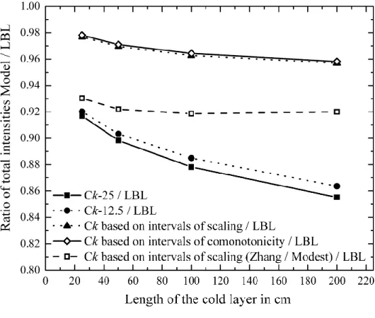
assessed against LBL calculation in a case taken from Ref. [13]. Results of a Ck-12.5 model
and the spectral mapping method proposed by Zhang and Modest in [13], based on the arbitrary
cut-off on scaling coefficients ucut-off = 10, are also provided for completeness. The two cells
contain the same gas, 20% H2O, 80% N2 at atmospheric pressure. The hot layer is at 2000 K and its length is 50 cm, and the cold layer is at 300 K and its length varies. Calculations are
which are used for comparisons with LBL calculations. These intensities are evaluated at the
cold side. Results are shown in Figure 8.
Figure 8. Comparison of several spectral mapping methods
From the results shown in Figure 8, the following conclusions can be drawn:
1/ Splitting the 25 cm-1 narrow band into two contiguous subintervals (yielding the Ck-12.5 solid circles) does not improve the approximation significantly compared to the Ck-25 method
(solid squares).
2/ Using intervals of scaling or comonotonicity clearly yields a high gain in terms of accuracy,
with errors reduced in the present case by a factor 4 when either the grouping scheme based on
scaling or comonotonicity described in this work are used. At identical computational costs,
spectral mapping methods have the potential to improve significantly the accuracy of the
case, the model based on intervals of comonotonicity has a slightly higher accuracy than the
model based on intervals of scaling. The spectral scaling method proposed by Zhang and
Modest also improves the accuracy of narrow band calculations, but can clearly not compete in
the case considered here with the two other grouping schemes described in this paper.
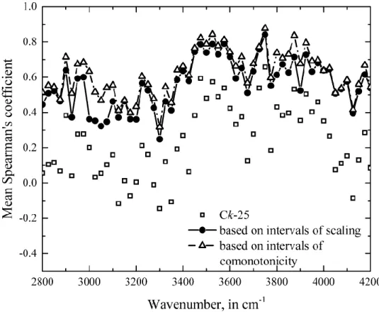
Finally, Figure 9 depicts mean Spearman’s coefficients calculated over narrow bands. Spearman’s coefficient is a measure of dependence [20] and characterizes the non-linear dependence between sets of values / random variables. The Ck / CKD model assumes this
coefficient to be 1. A null value of Spearman’s coefficient indicates complete statistical
independence. Negative values can be observed when high values in a sequence are associated
with low values in the other sequence, in which case variables are called counter-monotonic.
Over a narrow band , and for two thermophysical states as defined in section 2, Spearman’s coefficient can be calculated as [24]:
1 2
1 2 SP 1 2 1 , 12 g g d 3
(8)One can readily confirm that when spectra follow rigorously the implicit equation associated
with so-called “correlated” models, this coefficient is actually 1. In the modern statistical
literature [20], a Spearman’s coefficient equal to 1 characterizes comonotonic variables.
Over sub-intervals, one can similarly define group Spearman’s coefficients by simply replacing
the full band by the interval
ui , where u is the quantity assumed to be fixed over the i spectral interval and that can either represent a constraint on scaling or comonotonicity. It isthen possible to calculate an average value by weighting the Spearman’s coefficients over the
groups by the fraction of the interval associated with each group. In the case of two groups, as
1 2 1 2 1 2 1 2 SP SP,1 SP,2 1 2 1 2 SP, 1 2 , , , 1 , 12 3 i i i i i u u u g u g u d u
(9)These averaged Spearman’s coefficients SP
1, 2
are plotted in Figure 9 for the same case as for Figure 8 and for the two grouping schemes discussed in this paper (Modest and Zhang’stechnique is not considered). For the Ck model, Spearman’s coefficients were calculated from
Eq. (8): low and even negative values are observed. This explains why the Ck / CKD method
provides poor predictions in this high temperature gradient case, since the so-called “correlation” assumption is clearly inappropriate in this situation. Using the two grouping techniques described in this paper leads to higher values of averaged Spearman’s coefficients
1 2
SP ,
, which explains why the radiative transfer results of Figure 8 are more in accordance with LBL calculations when these grouping schemes are used than with the narrow
band Ck / CKD.
Notice also that averaged Spearman’s coefficients are slightly higher in the comonotonic case
than with scaling, which proves that the method to construct intervals of comonotonocity
actually improves the monotonic relationship between spectral values over the groups.
Furthermore, increasing the number of groups provides averaged Spearman’s coefficients that
approach unity: the relatively small values observed here are due to the choice of only two
groups. Finally, observing distinct values for the sets of Spearman’s coefficients proves that the
two techniques, based on intervals of scaling or comonotonicity, yield overlapping though
Figure 9. Comparison of averaged Spearman’s coefficients for several spectral methods
5. CONCLUSION AND PERSPECTIVES
The method described in the present note to construct intervals of comonotonicity: 1/ is simple
to understand and use, 2/ does not require an iterative process in the case of two-cell problems
(its extension to more general situations is kept as future work), and 3/ can be applied over any
band width, from narrow bands up to the full spectrum. It was shown to provide accurate
predictions of radiative intensities in situations representative of IR plume signature
configurations, a problem widely recognized as among the most complicated in band model
theory. Comparisons with a Ck / CKD model based on intervals of scaling were also described
and shown to provide a similar accuracy.
In addition, the method presented in this paper can be applied to atmospheric problems
requiring accurate treatment of gaseous absorption, such as for radiative forcing calculations or
two thermophysical states including temperatures of 300 and 1500 / 2000 K. However,
atmospheric applications cover a narrower range of temperature. In this respect, Fu and Liou
[22] have presented g-g plots for atmospheric conditions (temperature range between 245 and
300 K) and shown that the temperature effect produces more blurring. The degree of blurring
is then weaker for atmospheric applications, with points less scattered around the diagonal line
in the g-g plot. The building of intervals of comonotonicity should then be easier to define,
leading to reduced calculations times. The approach presented in this study is then a promising
method to improve the k-distribution and to reduce errors associated with the Ck / CKD
assumptions between atmospheric levels.
Finally, one can notice that no application of the Godson-Weinreb-Neuendorffer’s (GWN)
method [1] or use of effective scaling factors (see Ref. [24], in which a detailed analysis can be
found) was considered in this paper. Such comparisons are scheduled as future work together
with a comprehensive comparison of the two present techniques, extended to more than two
cells, with the Mixture l-Distribution approach (MLD) viz. the l-distribution method [25] applied to intervals of scaling.
AKNOWLEDGEMENTS
This work has been supported by the Programme National de Télédétection Spatiale (PNTS,
REFERENCES
[1] YOUNG SJ. Band model theory of radiation transport, The Aerospace Press, 2013. ISBN:
978-1-884989-25-4.
[2] WYATT PJ, STULL VR, PLASS GN. Quasi-random model of band absorption, JOSA
1962;52:1209-1217.
[3] LUDWIG CB, MALKMUS W, REARDON JE, THOMPSON JAL. Handbook of infrared
radiation from combustion gases, R GOULARD and JAL THOMPSON, eds, NASA SP-3080,
1973.
[4] VITKIN EI, KABASHNIKOV VP, KMIT GI. New method of calculating the infrared
emission of nonuniform volumes of molecular gases, Zhurnal Prikladnoi Spektroskopii
1979;30:686-693.
[5] KHODYKO YV, VITKIN EI, KABASHNIKOV VP. Methods of calculating
molecular-gas radiation on the basis of spectral-composition modelling, Inzhenerno-Fizicheskii Zhurnal
1979;36:204-217.
[6] KHODYKO YV, KUSKOV AA, ANTIPOROVICH NV. Multigroup method for the
calculation of selective IR radiation transfer in nonhomogeneous media, Zhurnal Prikladnoi
Spektrskopii 1986;46:449-455.
[7] LEVI DI LEON R, TAINE J. A fictive gas-method for accurate computation of
low-resolution IR gas transmissivities: application to the 4.3 µm CO2 band, Revue Phys. Appl. 1986;21:825-831.
[8] BHARADWAJ SP, MODEST MF. A multiscale Malkmus model for treatment of
[9] SOUFIANI A, ANDRE F, TAINE J. A fictitious-gas based statistical narrow-band model
for IR long-range sensing of H2O at high temperature, JQSRT 2002;73:339-347.
[10] WEST R, CRISP D, CHEN L. Mapping transformations for broadband atmospheric
radiation calculations, JQSRT 1990;43:191-199.
[11] BENNARTZ R, FISCHER J. A modified k-distribution approach applied to narrow band
water vapor and oxygen absorption estimates in the near infrared, JQSRT 2000;66:539-553.
[12] DOPPLER L, PREUSKER R, BENNARTZ R, FISCHER J. k-bin and k-IR: k-distribution
methods without correlation approximation for non-fixed instrument response function and
extension to the thermal infrared – applications to satellite remote sensing, JQSRT
2014;133:382-395.
[13] ZHANG H, MODEST MF. Multi-group full-spectrum k-distribution database for water
vapour mixtures in radiative transfer calculations, IJHMT 2003;46:3593-3603.
[14] ANDRE F, HOU L, ROGER M, VAILLON R. The multispectral gas radiation modeling:
a new theoretical framework based on a multidimensional approach to k-distribution methods,
JQSRT 2014;147:178-195.
[15] ANDRE F, HOU L, SOLOVJOV V.P. An exact formulation of k-distribution methods in
non-uniform gaseous media and its approximate treatment within the Multi-Spectral
framework, Eurotherm Conference N°105: Computational Thermal Radiation in Participating
Media V, 1-3 Avril 2015, Albi, France.
[16] ANDRE F, VAILLON R, GALIZZI C, GUO H, GICQUEL O. A multi-spectral reordering
technique for the full spectrum SLMB modeling of radiative heat transfer in nonuniform
[17] ANDRE F, VAILLON R. The multi-spectral reordering (MSR) technique for the narrow
band modeling of the radiative properties of non-uniform gaseous paths: the
correlated/uncorrelated approximations, Journal of Physics: Conference Series 369, 2012.
[18] HU H, WANG Q. Improved MSMGFSK models apply to gas radiation heat transfer
calculation of exhaust system of TBCC, JHT 2017 ;139,012702-1-11.
[19] HU H, WANG Q. Improved spectral absorption coefficient grouping strategy of wide band
k-distribution model used for calculation of infrared remote sensing of hot exhaust systems,
JQSRT 2018;213:17-34.
[20] NELSEN R.B. An introduction to Copulas - Second Edition, Springer series in statistics,
Springer, 2006.
[21] RIVIERE Ph, SOUFIANI A, TAINE J. Correlated-k fictitious gas model for H2O infrared
radiation in the Voigt regime, JQSRT 1995;53:335-346.
[22] FU Q, LIOU KN. On the correlated-k distribution method for radiative transfer in
nonhomogeneous atmospheres, Journal of Atmospheric Sciences 1992;49:2139-2156.
[23] ROTHMAN LS, GORDON LE, BARBER RJ, DOTHE H, GAMACHE RR, GOLDMAN
A, PEREVALOV VI, TASHKUN SA, TENNYSON J. HITEMP, the high-temperature
molecular spectroscopic database, JQSRT 2010;111:2139-2150.
[24] ANDRE F. Effective scaling factors in non-uniform gas radiation modeling, JQSRT
2018;206:105-116.
[25] ANDRE F. The l-distribution method for modeling non-gray absorption in uniform and non-uniform gaseous media, JQSRT 2016;179:19-32.