HAL Id: hal-02444133
https://hal.archives-ouvertes.fr/hal-02444133
Submitted on 17 Jan 2020
HAL is a multi-disciplinary open access archive for the deposit and dissemination of sci-entific research documents, whether they are pub-lished or not. The documents may come from teaching and research institutions in France or abroad, or from public or private research centers.
L’archive ouverte pluridisciplinaire HAL, est destinée au dépôt et à la diffusion de documents scientifiques de niveau recherche, publiés ou non, émanant des établissements d’enseignement et de recherche français ou étrangers, des laboratoires publics ou privés.
Impact of Maize Roots on Soil-Root Electrical
Conductivity: A Simulation Study
Sathyanarayan Rao, Félicien Meunier, Solomon Ehosioke, N. Lesparre,
Andreas Kemna, Frédéric Nguyen, Sarah Garré, Mathieu Javaux
To cite this version:
Sathyanarayan Rao, Félicien Meunier, Solomon Ehosioke, N. Lesparre, Andreas Kemna, et al..
Im-pact of Maize Roots on Soil-Root Electrical Conductivity: A Simulation Study. Vadose Zone
Journal, Soil science society of America - Geological society of America., 2019, 18 (1), pp.190037. �10.2136/vzj2019.04.0037�. �hal-02444133�
Impact of Maize Roots on
Soil–Root Electrical Conductivity:
A Simulation Study
Sathyanarayan Rao, Félicien Meunier, Solomon Ehosioke,
Nolwenn Lesparre, Andreas Kemna, Frédéric Nguyen,
Sarah Garré, and Mathieu Javaux*
Electrical resistivity tomography (ERT) has become an important tool for studying root-zone soil water fluxes under field conditions. The results of ERT translate to water content via empirical pedophysical relations, usually ignoring the impact of roots; however, studies in the literature have shown that roots in soils may actually play a non-negligible role in the bulk electrical conductivity (s) of the soil–root continuum, but we do not completely understand the impact of root segments on ERT measurements. In this numerical study, we coupled an electri-cal model with a plant–soil water flow model to investigate the impact of roots on virtual ERT measurements. The coupled model can produce three-dimensional simulations of root growth and development, water flow in soil and root systems, and electrical transfer in the soil–root continuum. Our electrical simulation illus-trates that in rooted soils, for every 1% increase in the root/sand volume ratio, there can be a 4 to 18% increase in the uncertainty of s computed via the model, caused by the presence of root segments; the uncertainty in a loam medium is 0.2 to 1.5%. The influence of root segments on ERT measurements depends on the root surface area (r = ?0.6) and the s contrast between roots and the soil (r = ?0.9), as revealed by correlation analysis. This study is important in the context of accurate water content predictions for automated irrigation systems in sandy soil.
Abbreviations: 3D, three-dimensional; ERT, electrical resistivity tomography.
Understanding root water uptake
and the associated nutrients is critical for crop management but remains a challenging task because of the inherent difficulty in making and taking observations inside soils (de Dorlodot et al., 2007). Geophysical moni-toring of root-zone soil moisture has received much interest in past decades as a way to tackle this challenge. One such method is ERT, which aims at retrieving the two- or three-dimensional distribution of s or its inverse (electrical resistivity) in the soil from electric resistance measurements at discrete electrode locations (Beff et al., 2013). The s is thus related to the property or state variable of interest, such as the soil water content (q), the porosity, the electrical conductivity of the soil fluid (sw), the temperature, or the mineral composition (Friedman, 2005). This is calculated through a proper pedophysical relation-ship (e.g., quantifying s as a function of q). In cropped fields, ERT has been increasingly used for monitoring q (Michot et al., 2003; Srayeddin and Doussan, 2009; Garré et al., 2013; Cassiani et al., 2015; De Carlo et al., 2015; Brillante et al., 2016; Vanella et al., 2018). More recently, ERT-estimated water content has been used for phenotyping root systems at the field scale (Whalley et al., 2017). Whalley et al. (2017) monitored changes in the s of the soil root zone under drying conditions at different soil depths, which acted as a proxy for root activity. However, the bulk electrical conductivity (sbulk) of a vegetated soil potentially containing roots depends not only on q but also on the roots and their impact on the soil structure (Garg et al., 2019). For example, a recent pot experiment showed that diseased and healthy roots in the soil could generate different ERT measurements (Corona-Lopez et al., 2019). In some field experiments, different pedophysical relationships for soils with and without roots have been observed (Werban et al., 2008; Michot et al., 2016; NiCore Ideas
• The impact of roots on bulk electri-cal conductivity was studied using a modeling approach.
• The presence of roots affects petro-physical relations.
• The effect of roots is more pro-nounced in sandy soil than in loamy soil.
• Root surface and soil–root electrical contrast affect ERT measurements the most.
S. Rao and M. Javaux, Earth and Life Institute– Environmental Sciences, Univ. catholique de Louvain, Louvain-la-Neuve, Belgium; F. Meu-nier, Computational and Applied Vegetation Ecology Lab., Ghent Univ., Ghent, Belgium; S. Ehosioke and F. Nguyen, Applied Geophysics, Univ. de Liège, Chemin des Chevreuils 1, 4000 Liege, Belgium; N. Lesparre, Lab. d’Hydrologie et Géochimie de Strasbourg, Univ. of Stras-bourg, l’Ecole et Observatoire des Sciences de la Terre/l’Ecole nationale du génie de l’eau et de l’environnement de Strasbourg, Centre national de la recherche scientifique unité mixte de recherche 7517, 1 Rue Blessig, 67084 Strasbourg, France; A. Kemna, Dep. of Geo-physics, Univ. of Bonn, Meckenheimer Allee 176, 53115 Bonn, Germany; S. Garré, Univ. de Liège, Gembloux Agro-Bio Tech, TERRA Research and Teaching Center, Passage des déportés 2, 5030 Gembloux, Belgium; M. Javaux, Institute for Bio- and Geosciences, Agrosphere Institute, Forschungszentrum Juelich GmbH, Juelich, Germany. *Correspon-ding author ([email protected]).
Received 15 Apr. 2019. Accepted 21 Aug. 2019. Supplemental material online.
Citation: Rao, S., F. Meunier, S. Ehosioke, N. Lesparre, A. Kemna, F. Nguyen, S. Garré, and M. Javaux. 2019. Impact of maize roots on soil–root electrical conductivity: A simu-lation study. Vadose Zone J. 18:190037. doi:10.2136/vzj2019.04.0037
Original Research
© 2019 The Author(s). This is an open access article distributed under the CC BY-NC-ND license (http://creativecommons.org/licenses/by-nc-nd/4.0/).
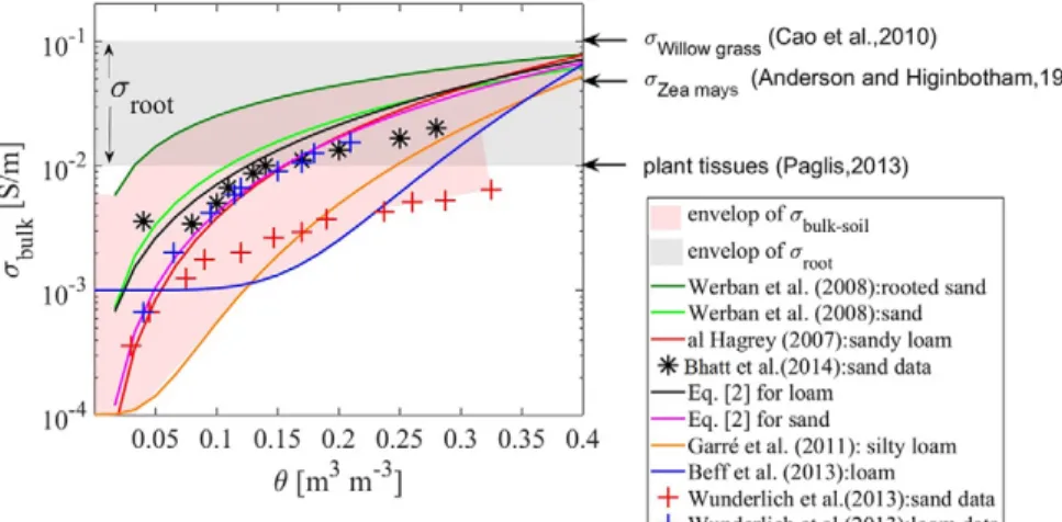
et al., 2018). However, in lysimeter experiments, studies showed that pedophysical function was time invariant, despite ongoing root growth (Garré et al., 2011). In Fig. 1, we show the envelope of the sbulk values of soil without roots (sbulk-soil) and the envelope of the s of root segments (sroot) as reported by several researchers. Figure 1 shows that the contrast between sroot and sbulk-soil is a function of plant species in addition to the soil bulk properties or state variables and indicates that roots could have a measurable but variable impact on ERT measurements.
For a given species, sroot is generally a function of root anat-omy, which can be related to root age, root order, or root diameter. In their study, Anderson and Higinbotham (1976) found that older maize (Zea mays L.) root segments are electrically more con-ductive than younger roots. Their study was performed on excised root segments. They showed that the outer layer of the root seg-ment (cortex) has very low electrical resistance (?50 kW) in the radial direction compared with the axial direction (?600 kW). By treating the cortex and stele as concentric parallel conductors, the reported resistances, when converted into conductivities, are on the order sroot ? 0.05 S m−1. However, the electrical behavior
of intact root segments embedded in the soil might be differ-ent from that of excised segmdiffer-ents. Another study by Cao et al. (2010) reported that root electrical resistance could be related to root properties such as surface area, the number of lateral roots, and root length. Studies on poplar (Populus sp.) roots showed that the sbulk of the soil–root medium may increase or decrease with an increase in root mass density, depending on the age of the plant (al Hagrey, 2007; Zenone et al., 2008; Mary et al., 2016). In addition, some studies have found a correlation between the root length or mass density and electrical resistivity obtained through ERT (Amato et al., 2009; Rossi et al., 2011). Along with root geo-metrical properties such length, surface area, or mass density, the electrical contrast between roots and the soil also plays a role in influencing ERT results. However, it is not clear what proportion of the electrical signature of roots that can be seen in the ERT measurements can be attributed to each of the root parameters (e.g., electrical contrast, root length, surface area, and volume density).
Beyond the impact of sroot, root-related processes such as water uptake, exudation, or solute uptake will also affect the
electrical properties of the rhizosphere (i.e., the soil zone in close proximity to the root segments), thereby affecting the contrast between sroot and sbulk-soil. Recent ERT experiments on orange [Citrus × sinensis (L.) Osbeck] orchard fields suggest that ERT results are more sensitive to root water uptake patterns (Vanella et al., 2018) than to resistive lignified roots. Performing such experi-ments is, however, costly and time consuming and is difficult to reproduce for various species and soil types, hence the need for modeling. Al Hagrey and Petersen (2011) previously studied the impact of roots on ERT imaging by using a root growth model (Wilderotter, 2003) but ignored the inherent heterogeneity of sroot and sbulk-soil. To understand the effect of root system connectiv-ity and their impact on sbulk, a model where functional roots are explicitly represented is needed. Explicit root representations pro-vided by an unstructured finite element mesh have been studied for water and nutrient uptake processes (Wilderotter, 2003; Tournier et al., 2015). In this study, we have extended it to ERT forward simulation coupled to a plant–soil water flow model and a realistic complex root system architecture.
The objective of this study was to investigate the impact of root segments and root water uptake on the effective soil–plant s. Specifically, we wanted to quantify the effects of soil–root contrast, plant growth, and root water uptake on the pedophysical relations.
6
Materials and Methods
To achieve our objectives, we developed a soil–plant model that combines electric and hydraulic dynamics and applied it to generate virtual rhizotron experiments. A rhizotron is a thin con-tainer (typically around 2 by 20 by 40 cm) filled with a growth substrate in which plant roots develop, allowing observation of the development of the root system architecture and sometimes the substrate water content (Garrigues et al., 2006; Ahmed et al., 2018) and can thus be used to investigate how soil heterogeneity affects root growth and uptake (e.g., Bauke et al., 2017). In this study, the soil–root system was modeled at a fine spatial resolu-tion for the roots via an unstructured mesh for ERT forward simulation. The virtual environment allowed us to account for root architecture, soil water redistribution, soil heterogeneity,
Fig. 1. Comparison of soil and root electrical conductivity (ssoil and sroot, respectively). The envelopes of ssoil (some with and some with-out roots) and sroot are shown as shaded areas (Paglis, 2013; Bhatt and Jain, 2014).
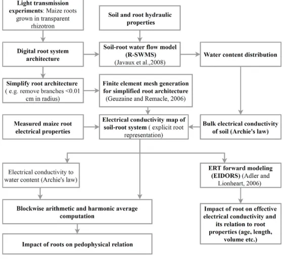
root-specific electrical properties, root growth, and transient transpiration. Figure 2 summarizes the various steps of this mod-eling process as a flowchart.
The Root Growth Experiment
and the Soil–Plant Water Flow Model
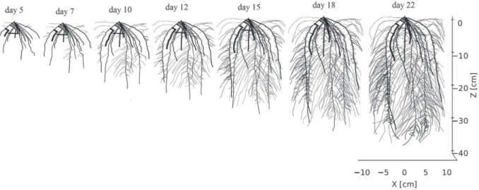
The two-dimensional root architecture (see Fig. 3) was extracted from real experiments on a rhizotron with 21-d-old maize by the root image analyzing tool smartroot (Lobet et al., 2011; Lobet and Draye, 2013). We used a 5- to 21-d-old root system for our simulations. Because root growth was monitored every day, ages were easily assigned to each root segment. In these experi-ments, the rhizotrons were weighed daily, thereby allowing us to estimate the average transpiration rates.
The rhizotrons measured 22 by 2 by 42 cm (the correspond-ing reference axes are −11 cm £ x £ 11 cm, −1 cm £ y £ 1 cm, and −40 cm £ z £ 2 cm). We considered two soil types: sandy and loamy, with the hydraulic properties represented by Mualem– van Genuchten equations (van Genuchten, 1980) in Table 1. Hydraulic parameters for both soils were derived from Carsel and Parrish (1988).
The soil–plant water flow model R-SWMS (Javaux et al., 2008) was used to estimate the evolution of root water uptake, soil water flux, and the q distributions in the rhizotrons. R-SWMS uses the finite element method on a regular uniform grid to solve Richards’ equation to simulate three-dimensional (3D) water flow in the soil: ( ) Sink h z h h K K K t x x y y z z æ ö é ¶ + ù æ ö ¶q ¶ ç ¶ ÷ ¶ ç ¶ ÷÷ ¶ ê ú = ×èçç ÷÷ø+ ×ççç ÷÷+ ×ê ú -¶ ¶ ¶ ¶ è ¶ ø ¶ ë ¶ û [1]
where q is the volumetric soil water content (cm3 cm−3), h is the
matrix head (cm), K is the isotropic hydraulic conductivity (cm d−1), Sink is the sink term for root water uptake (cm3 cm−3 d−1),
and x, y, and z are the spatial coordinates; the dot represents divergence. The sink term is estimated on the basis of a weighted averaged of the uptake fluxes in each soil voxel.
The water fluxes into and toward the roots were calculated via a finite difference method in the root system network based on soil and root water potential distributions and the transpiration rate. The transpiration rate increased with root growth. Each root seg-ment was characterized by its radial and axial hydraulic properties,
Fig. 2. Flow chart for simulation of the virtual rhizotron drying experiment. First, a simulation of root water uptake and root growth of a maize plant in a rhizotron is run with a soil–plant water flow model (R-SWMS; Javaux et al., 2008), which generates maps of soil water distribution (q) and development of root architecture. These distributions are then transformed into detailed electrical conductivity (s) maps through bio- or pedophysical relationships. Third, these distributions are used to simulate a virtual electrical resistivity tomography (ERT) measurement to obtain
which developed with root segment age. Experimentally mea-sured maize root hydraulic conductivity values were used in the R-SWMS model, in which they were age and type dependent (Doussan et al., 2006; Couvreur et al., 2012). The total root length per unit of volume in the R-SWMS simulation was 0.06, 0.22, 0.66, 1.1, and 1.61 cm cm−3 on Days 5, 10, 15, 18, and 21,
respec-tively. In a typical field, mature root density can reach values of 1 cm cm−3, especially in the topsoil (Gao et al., 2010).
Root growth was simulated by updating the root system archi-tecture at each time step between the beginning (Day 5) and the end (Day 21) of the simulation. The same architecture develop-ment pattern was used for sand and loam. We imposed a sinusoidal day–night transpiration as a root boundary condition, with daily transpiration progressively increasing between the beginning (Day 5, 5 cm3) and the end of the simulation (Day 21, 30 cm3), which
corresponds to the transpiration rates experimentally observed in greenhouse experiments for similar sized plants (Lobet et al., 2011). The initial soil condition was hydrostatic equilibrium with a saturated soil at the bottom of the rhizotron (corresponding to the experimental conditions), and root water uptake was the only source or sink term that allowed the total water content to change. We ignored root exudation and assumed that solute uptake was proportional to the soil solute concentration (i.e., passive uptake) (Hopmans and Bristow, 2002), allowing us to assume a uniform concentration distribution in the liquid solute. Therefore,
no change in s caused by solute buildup in the rhizosphere was considered in our simulations.
Electrical Properties of Plant Root Tissues and Soils
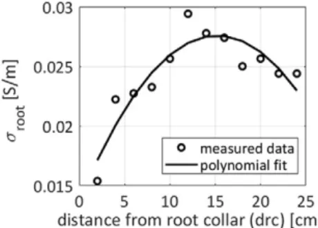
To get insight into the maize roots’ electrical properties, we followed the method of Ehosioke et al. (2018), who designed spe-cific experiments on intact root segments, where the primary and brace roots from maize plants grown in the laboratory were identified and separated. Roots were then thoroughly washed with demineralized water and dried with absorbent tissue. The electrical resistance of the root segments was measured with a digital multimeter (Fluke 8022A, Fluke Corporation) and were converted into sroot by approximating the root segment as having a cylindrical geometry, similar to the method of Cao et al. (2010). The measurement direction of root segments in Cao et al. (2010) was from the root apex toward the root collar, but it was in the opposite direction in the case of the experiment of Ehosioke et al. (2018). In our study, we used the variations of sroot as a func-tion of each segment’s distance from the root collar (Fig. 4). The digital maize roots in ERT forward modeling were ?3 wk old, although the brace roots develop only after several weeks in a real maize plant; hence, the brace root data were not included in our model. Figure 4 shows the experimental data of sroot as a function of root age for maize plants. We observed a gradual increase in sroot for intact maize root segments as the distance from the segment to the root collar increased. For each root segment, the Euclidean distance between the midpoint of that segment and the seed location (x = 0, z = 0) was taken as the dis-tance to the root collar and was assigned a sroot value according to the polynomial fit, as shown in Fig. 4. However, in our virtual root simulation, the distance to the root collar could be >25 cm in older plants (Fig. 3), for which we do not have corresponding sroot values in the measurement data. Hence sroot for a distance to the root collar of >25 cm was taken as sroot at a distance to the root collar of 25 cm.Fig. 3. Root architectural development shown at different times. A digitized root system was generated by smartroot software (Lobet et al., 2011). The thickness of each root segment is plotted proportional to its radius.
Table 1. Soil hydraulic properties.†
Soil qr qs a n Ks l
—— cm3 cm−3 —— cm−1 cm d−1
Sand 0 0.35 0.05 2 100.24 0.5
Loam 0.078 0.435 0.036 1.56 25 0.6
† qr, residual water content, qs, saturated water content; a, n, and l, shape
pa-rameters in van Genuchten–Mualem equations; Ks, saturated soil hydraulic conductivity.
To transform q maps into s maps, we used Archie’s law (Archie, 1942) with an additional term for the surface conductiv-ity of the solid phase, ssurface, which is assumed to act in parallel (Waxman and Smits, 1968). The relation between q and sbulk-soil for unsaturated soil, where Archie’s fitting parameters (m and d) vary for different types of soil (Friedman, 2005), is
1
bulk-soil w surface
s = s n Sm d+Sd-s [2] where S is the degree of water saturation (S = q/n), n is the poros-ity of the soil (which is assumed to be equal to the saturated water content, qs), sbulk-soil is the bulk electrical conductivity of the soil medium without considering roots, sw is the conduc-tivity of soil fluid phase, and ssurface is the surface s of the solid phase of the soil. Sand typically has very low surface conductivity (?10−5 S m−1); for loam, we assumed the surface conductivity of
the solid phase to be 0.015 S m−1 (Brovelli and Cassiani, 2011).
For Archie’s fitting parameters, we used the typical values d = 2 and m = 1.3 (e.g., Werban et al., 2008). In the rhizotron, sbulk-soil also depends on the sw of the nutrient solution used to grow the plants. We assumed the s of the nutrient solution to be 0.2 S m−1
and chose n as 0.35 (sand) or 0.435 (loam) to be in the same range as seen in the other observed pedophysical models (Fig. 1). We refer to sbulk-soil as the soil bulk electrical conductivity when no roots are present; sbulk is used for studies or datasets where both roots and soil are present.
Note that extremely low values of conductivity in sand (?5 × 10⁻⁹ S m−1) can arise and would need additional mesh
refine-ment in the forward finite elerefine-ment mesh (see below) in regions where there were large conductivity gradients to obtain accurate results. To avoid this scenario and to maintain accuracy, we set a limit of 0.0001 S m−1 as the lowest possible conductivity value.
Meshing the Root Architecture
For the electrical simulation, we generated finite element meshes for the specific root geometry. In the finite element mesh,
either a sroot or sbulk-soil q value was assigned to each element (tet-rahedron). The primary maize roots in our simulation had a mean radius of ?0.025 cm, which is small compared with the dimen-sions of the rhizotron (20 by 1 by 42 cm), requiring a very high spatial resolution for roots in the forward finite element mesh.
To generate a 3D mesh with a high spatial resolution for the roots but a manageable computational load (<1 million tetrahe-drons), we needed to simplify the root system while maintaining a realistic representation of the main structure. First, we removed extremely fine root hairs and root branches that were <0.01 cm in radius, assuming that such roots have a negligible effect on the voltage measurements. In addition, nearly parallel secondary root branches with a distance of less than double the root radius between them were combined and treated as a single branch. This procedure reduced the total root length in the finite element mesh compared with a real plant. Hence, to preserve the root volume, which we assumed to be the most important factor, in the finite element mesh with the actual measurements we had to increase the mean radius of the root segments. In addition, we discretized each root segment radius in the finite element mesh into two possible values, where all primary roots had one radius but all secondary roots had half the radius of the primary roots; in reality, each segment had unique radii. This simplification affected only the electrical forward model (roots were explicit 3D structures in the electrical mesh) and not the water flow model (roots were treated as a network with no volume in the water flow grid), where we used digitized roots that had identical features (radii and number of segments) to those in the rhizotron experiments.
We compared the time evolution of root volume, total root length, and mean root radius in the finite element mesh with the actual plant (Fig. 5). The root volume in the finite element mesh matched that of the real plant (Fig. 5a). The total root length in the finite element mesh matched the measurements in a younger plant only (Fig. 5b). In older plants, we lost around 50% of the root length through the root simplification procedure. The sim-plified root architecture represented segments with a mean radius, as shown in Fig. 5c.
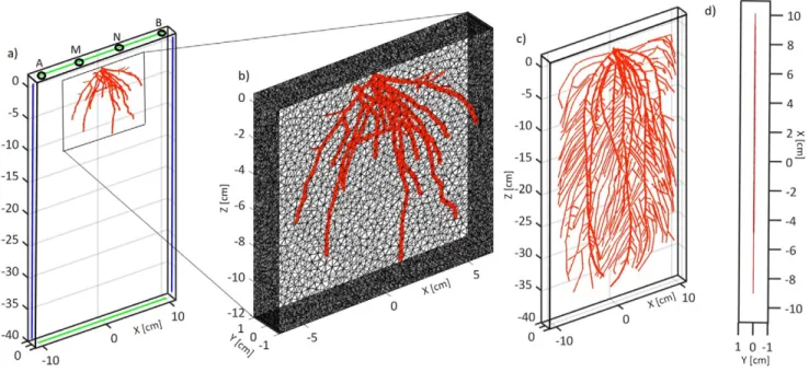
The finite element model of the simplified root architecture at Day 5 is shown in Fig. 6. The 3D finite element mesh in Fig. 6c was generated from the simplified root architecture by gmsh software (Geuzaine and Remacle, 2009). Figures 6a and 6b show the simpli-fied architecture at Day 5; Fig. 3 shows the original architecture of a real plant at different times. By comparing these two figures at Day 5, we see that the overall skeleton of the root system and its volume were preserved, although its radii were modified to suit the computational speed. We assumed that root mass density (or root volume) played a bigger role than root length density in affecting the flow of electrical current and hence we prioritized preserving the root volume and, to some extent, the architecture rather than preserving the actual root length and radius, which were modified in the mesh through merging closely adjacent segments. In addi-tion, preserving root radii and root lengths would require a very refined grid and hence would be computationally intensive.
Fig. 4. Measurement data on the electrical conductivity of maize roots (sroot) vs. distance from the root collar. The quadratic fit is shown as a solid line, and the measurement data are represented at discrete locations as circles (primary roots). The polynomial fit sroot = −5.5 ´ 10−5(drc2) + 0.0018drc + 0.0137, where drc is
dis-tance to the root collar, was used in the model simulations. The black solid curve represents the data incorporated in the electrical resistivity tomography electrical resistivity tomography (ERT) forward model-ing: 0.0154 < sroot < 0.03 S m−1.
We also generated additional synthetic data by increasing the mean root radius by factors of two and three (increasing the root volume by fourfold and ninefold). The original mean radii of the root segments in the finite element mesh that matched the exper-imental volume are shown in Fig. 5d (red squares). Thickening the roots increased the root volume while keeping the root length intact. With seven different root ages (seven different root lengths; see Fig. 3) and three different root radii—actual (Fig. 5d), double of actual, and triple of actual—we had 21 different radii and vol-umes to be analyzed.
Electrical Resistivity Forward Modeling
We used the finite element based software EIDORS (Adler and Lionheart, 2006) to solve the ERT forward simulation for the generated finite element meshes. The ERT forward simulation solved for the resulting voltages of an electric current of density
Je, injected into a medium of s, given the proper boundary condi-tions. The equations governing the physics of electrical resistivity forward modeling are derived from Maxwell’s equations for a direct current. Consider a region W bounded by its boundary, dW. The electric field E in W is related to the scalar electric potential f through the gradient operation E = −Ñf. By applying the con-servation of electric charge for a source-free region (Ñ×Je = 0) and Ohm’s law (Je = sE), we obtain the governing equation for ERT inside the medium (also known as the Laplace equation):
( ) 0
Ñ× sÑf = [3]
The injected current density is specified by the Neumann boundary conditions at the current injecting electrode locations, which are usually located in dW:
Fig. 5. (a) Root volume vs. root age and (b) root length vs. root age as simulated in the finite element mesh (red squares) or light trans-mission images (black circles), and (c) mean radius vs. root age in the finite element mesh (red squares) or measurements (black circles).
Fig. 6. (a) Finite element model of the virtual rhizotron in EIDORS on Day 5. The vertical line electrodes used to compute the effective electrical con-ductivity (seffx) are shown in blue and the horizontal line electrodes used to compute seffz are shown in green with the mesh hidden. The black circle
at the surface denotes the location of point electrodes, denoted by ABMN, used to compute sabmn. (b) Close-up view of a section of the forward finite element mesh; (c) model on Day 21 with the mesh hidden. (d) Top view of the finite element model on Day 21. The root tetrahedrons are shown in red.
e e
on the current injecting electrode on the sink electrode
0 elsewhere ˆ ˆ n n ì ü ï ï ï ï ï ï ¶f ï ï sÑf =s = -íï ýï ¶ ï ï ï ï ï ï î þ J J [4]
The voltage-measuring electrodes dictate the Dirichlet boundary conditions:
e e e
Z V
f+ J = [5]
where Ze is the contact impedance of the voltage-measuring elec-trodes (assumed to be 0.01 W in this work), Je is the current density given by Je = s(¶f/¶nˆ), Ve is the voltage (in V), and nˆ is the unit normal perpendicular to dW. Equations [3–5] are the governing equations for the ERT forward problem.
The ERT forward simulation finds voltage or apparent conductivity data by numerically solving Eq. [3–5] for a known distribution of s. The voltage data (Ve) can be converted to appar-ent conductivity data, namely that of an equivalappar-ent homogeneous medium, with an appropriate geometric factor for the electrodes. The apparent conductivity data measured between the line elec-trodes in the y = 0 plane (the green and blue lines in Fig. 6a) of each wall (top, bottom, left, and right) gives the effective electri-cal conductivity (seff) in the vertical and horizontal directions, denoted seffz and seffx, respectively. Similarly, apparent conduc-tivity measured between the surface quadrupoles (sabmn, black circles in Fig. 6a) gives the apparent conductivity. The electrical conduction model for the rhizotron is in three dimensions (the same as in the water uptake model in R-SWMS) with the follow-ing overall dimensions: −11 cm < x < 11 cm, −1 cm < y < 1 cm, and −40 cm < z < 2 cm.
Upscaled Electrical Properties
To get an insight into how a root-filled soil might differ from bare soil electrical properties, we divided the forward finite element mesh into smaller blocks measuring 2 by 1 by 2 cm and computed the Wiener upper and lower bounds of s (Wiener, 1912; Jougnot et al., 2018) or the volume-weighted arithmetic and harmonic mean of s within each block (Fig. 2) via Eq. [6] and [7], respectively:
i i i i i V V s s =
å
å
[6](
)
1 1 1 i i i i i V V -é s ù ê ú s = ê ú ê ú ë ûå
å
[7]where Vi and si are the volume and electrical conductivity of the ith tetrahedron within an averaging block. We also computed the volume-weighted arithmetic mean of water content computed from s (Archie’s law in reverse, as shown in Fig. 2):
i i i i i V V q q =
å
å
[8]The blockwise-computed arithmetic average of electrical conductivity assumes that the finite elements in each averaging
block are electrically connected in series, whereas the blockwise-computed harmonic average of electrical conductivity assumes the elements to be in parallel. In reality, we expect the true sbulk to be in between the blockwise-computed arithmetic and harmonic averages of s, depending on the structural properties of the roots and soil elements. The relationship between the collection of aver-aged data points from every averaging block and at all times (Days 5–21) will then approximately mimic the impact of roots at the block scale on sbulk, compared with Archie’s law applied in soils only (sbulk-soil). We also investigated the relationship between the effective properties (seffz andseffx) and volume-averaged (at the rhizotron scale) water content at different times.
Relative Change in Effective Conductivity
Caused by Root Segments
The computation of seff (seffz and seffx) and sabmn was repeated for two scenarios: (i) a medium with the soil and root system included and (ii) a medium with only the soil, as if the roots had the same s than the surrounding soil. The difference in seff between the root and soil indicates the specific impact of root segments on the electrical measurements. Similarly, the difference in sabmn between the root and soil indicates the specific impact of root segments on ERT measurements made by point electrodes at the surface rather than the effective properties.
We define a parameter describing the relative change in seff caused by the presence of root segments (dseff-rs), which is given by
eff-root eff-soil eff-rs eff-soil s - s ds = s [9]
where seff-root is the seff of the medium with both roots and soil and seff-soil is the seff of the medium with soil only.
Similarly, the relative change in sabmn computed by point electrodes caused by the presence of root segments is given by
abmn-root abmn-soil abmn-rs abmn-soil s - s ds = s [10]
where sabmn-root is the sabmn of the medium with both roots and soil and sabmn-soil is the sabmn of the medium with soil only.
We investigated the relative change in seff at different root ages and with varying soil types (soil and loam; see Table 1). Furthermore, the relative change in seff averaged across two per-pendicular directions (ádseff-rsñ) and dsabmn-rs are used as the parameters to assess the impact of roots in the following. We refer to ádseff-rsñ and dsabmn-rs as the roots’ electrical signature term. We also define a term describing the contrast in s between sroot
and sbulk-soil, computed by subtracting the mean of sbulk-soil from the mean ofsroot. Here, s contrast is a single number that is a func-tion of root age and soil type.
Scenario Analysis
We used the simulated synthetic data to achieve the objectives of this study, namely to find simulation-based answers to the ques-tion of how root length density, root volume density, root age, and
root radius relate to the root electrical signature terms. To answer this question, we assessed the dependence of ádseff-rsñ for each of the unique cases that corresponded to different root variables such as length, age, volume, surface area, s contrast, and radius. We investigate the dependence among these variables via correlation and principal component analysis.
6
Results
Bulk Electrical Conductivity as a Function
of Time and Soil Type
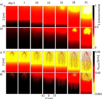
Simulations showed that the water saturation distribution patterns depended on the soil type (Fig. 7a and 7b). In loam, the normalized water saturation never dropped below 0.2, even on Day 21, whereas in sand, it reached almost zero (0.00034) on Day 21. The same day, when the water depletion reached its greatest, the maximum water saturation values were 0.4 in sand and 0.6 in loam. In sand, sroot was always larger than sbulk-soil (Fig. 7c). For loam, however, the contrast changed with time (Fig. 7d). Initially, in loam, sbulk-soil was larger than sroot; at intermediate times (Days 10, 12, and 15) at the top of the rhizotron, sbulk-soil was equal to sroot, and at the bottom of the rhizotron, sbulk-soil was larger than sroot. At the end (Days 18 and 21), in some regions sbulk-soil was less than sroot. On Day 21, sbulk-soil varied from 0.0001 to 0.0087 S m−1 in sand and from 0.0057 to 0.0407 S m−1
in loam.
Impact of Roots on Pedophysical Relationships
The harmonic and arithmetic blockwise averaged s data points and their corresponding water content at various times are shown as vertical bars in Fig. 8a and 8b, along with Archie’spedophysical relationship. The upper limit of the vertical bar rep-resents the maximum of the blockwise-computed arithmetic and harmonic averages of s; the lower limit represents their minimum. For each block (4 cm3), the actual effective small-scale
(centimeter-scale) s is supposed to be located within this range.
At a larger rhizotron spatial scale, we illustrate the relation-ship between seffz or seffx and the volume-averaged water content at various times in Fig. 8a and 8b. Both the effective properties at rhizotron scale and the averaged properties at small block scale deviated from Archie’s curve, and the deviation trends were differ-ent, as seen in Fig. 8a and 8b. In addition, the difference between the horizontal and vertical effective properties seffx and seffz indi-cate the macroscale anisotropy. For both soil types, the derived effective properties seffx and seffz lay below Archie’s curve defined at a lower scale because the dry soil acted as a barrier to the electri-cal current flow, thus decreasing the effective sbulk. The vertical effective property deviated more than that of the horizontal direc-tion because of horizontal layering developing in the s distribudirec-tion as a result of root water uptake (Fig. 8a and 8b). Current was there-fore affected more in the vertical direction than in the horizontal direction. For the loam medium, the anisotropic effect was less than that of the sand. In fact, ERT-obtained s data are known to have a spread around the pedophysical model fitted curve, as observed by Beff et al. (2013) and Garré et al. (2011). Our averag-ing results in Fig. 8a and 8b hint that this deviation in the s data around the pedophysical model could be caused by the presence of root segments.
In Fig. 8c and 8d, we show the deviations of seffz from Archie’s curve in sand and loam for three different scenarios: 1. Root water uptake with root segments: Here, we have Fig. 8c
and 8d as the forward s map.
Fig. 7. Volumetric water saturation (S) distribution in (a) sand
and (b) loam and its corresponding electrical conductivity (sbulk) maps in (c) sand and (d) loam in the Y = 0 plane at
2. Root water uptake without root segments: For this scenario, in Fig. 8c and 8d, we removed the root-specific electrical properties and assumed that the roots have the same s as the surrounding soil but retain the root water uptake pattern in the forward s map.
3. Homogeneous soil with root segments: For this case, we removed the pattern of sbulk-soil associated with water uptake by roots in Fig. 8c and 8d and replaced it with its spatial aver-age (homogeneous soil). The root-specific electrical properties were retained.
As the sroot values are generally higher than those of the dry soil, we see that the deviation is positive for the homogeneous sce-nario (red lines in Fig. 8c and 8d), whereas with root water uptake, the deviation is negative.
We find that the impact of root water uptake was slightly bigger than that of sroot only (the green and red lines, respectively, in Fig. 8c and 8d). However, the additional impact of roots when water uptake was considered was negligible (blue line), demonstrat-ing that root water uptake patterns were the main driver of these deviations. The presence of roots inside the depletion zone only marginally affected the electrical signature.
At small scales, removing root segments results in perfect agreement between blockwise averaged data and Archie’s curve (data not shown), as the difference between the two averages in Fig. 8a and 8b was caused only by root segments. This is because at block scale, there is no significant water content heterogeneity present and thus the average water content and average s (without roots) follow Archie’s curve. At large scales, though, the patterns generated by water uptake were more nonlinear and the average water content no longer related to the effective properties dictated by Archie’s pedophysical relationship. This illustrates how the rela-tionship between q and sbulk is scale dependent.
Roots’ Electrical Signature
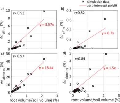
In Fig. 9, we compare ádseff-rsñ and dsabmn-rs with the root/ soil volume ratio as a percentage. They show a very high correla-tion both in sand and loam (r > 0.8). In general, the impact of roots in sand was greater than in loam, as seen by its higher slope. In Fig. 10, we examine the correlation of ádseff-rsñ with several root segment properties such as radius, surface area, volume, age, and soil–root electrical contrast. The root electrical signature terms depend more strongly on electrical contrast than on other
Fig. 8. (a,b) Comparison of Archie’s law (sbulk-soil) with blockwise-averaged electrical conductivity (áqñ) vs. blockwise-computed arithmetic average of electrical conductivity (ásavg-hmñ), blockwise-computed harmonic average of electrical conductivity (ásavg-amñ), and rhizotron-scale effective electrical conductivity in two perpendicular directions (seffx and seffz) in (a) sand and (b) loam. The error bar represents the Wiener bound values or the range of variation between savg-am and savg-hm. The water content corresponding to seffx and seffz were obtained by taking the volumetric average of the entire rhizotron. (c,d) Deviation of seffz from sbulk-soil as a function of root volume for three different scenarios in (c) sand and (d) loam.
parameters for the root water uptake case. By visual inspection of Fig. 10, we find that age and length varies with ádseff-rsñ in a similar fashion, whereas surface and volume form another group. The electrical contrast is an independent variable affecting the ádseff-rsñ. Correlation analyses indicate that root surface area and electrical contrast are the two main drivers of the electrical signa-tures of root systems in soils.
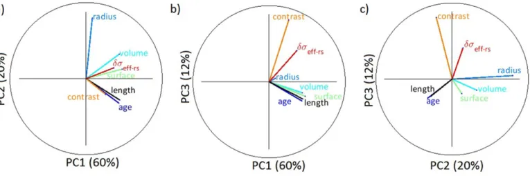
The results of principal component analysis (Fig. 11) con-firmed the multivariate dependence among different variables relating to root geometrical and electrical properties. The prin-cipal component analysis revealed that the first three prinprin-cipal components explained about 92% of the variability (Fig. 11). Principal Component 1, with 58% of the total variance, captured the variability of root system size (volume, surface, radius, and age), which correlated with electrical contrast and the electrical signature. In other words, large root systems tend to increase their electrical signature.
Principal Component 2 separated the various drivers of vari-ability into three groups. Age and length, which represent the extent of the root system, formed Group 1 and were negatively correlated with ád seff-rsñ. Radius made up Group 2 and was weakly correlated with ádseff-rsñ. Volume and surface, which rep-resent a combination of extension and thickness, formed Group 3 and correlated with ádseff-rsñ. Principal Component 3 captures a small part of the variation, where contrast and ádseff-rsñ are correlated and are independent of root system size.
Model Limitations
Here, we discuss the limitations of our modeling approach. First, we consider the limitations for the scenario where the process-based model described here is extended to model a real experiment. In agricultural fields as well as in the two-dimensional rhizotron, air-filled cracks can manifest in the soil, potentially influencing ERT measurements that our model does not account for; however, these could easily be integrated into the model. For future validation of the modeling results presented here in a real experiment, limitations in ERT such as bad electrode contact and other artifacts such as soil cracks can be combated through repeated measurements and adjust-ments during the course of the experiment, which are simpler to implement in a rhizotron experiment than in the field (Huck and Taylor, 1982).
Our model did not consider specific rhizosphere processes such as root exudation, which could also affect the water content estimates. In the model, we assumed that salt did not accumu-late near the roots but assumed passive solute uptake only with no active uptake, exclusion, or exudation. Although this has been observed experimentally under field conditions by Beff et al. (2013) and corresponds to a situation where the nutrient solution exactly fits the plants’ needs, the assumption is not necessarily always valid. Significant solute gradients may arise around roots through the processes mentioned above. If they were to occur, the forward conductivity map and hence the water content estimates could be impacted by such gradients.
In addition, roots can swell and shrink, causing air gaps that change spatially and temporally between soil and roots under field conditions (Carminati et al., 2009). Studies have found that maize roots in sandy loam have a root–soil contact surface of 40 to 60%
Fig. 9. Relative change in effective conductivity resulting in root segments compared with soil only (ádseff-rsñ) vs. root volume/soil volume ratio (black squares) in (a) sand and (b) loam. Relative change in apparent conductivity from root segments compared with soil only (dsabmn-rs) vs. the root vol-ume/soil volume ratio (black squares) in (c) sand and (d) loam. The red line represents the zero-intercept-constrained polynomial fit.
Fig. 10. Correlation plots of different root variables: radius, age, volume, surface area, length, and electrical conductivity contrast between root and soil (C), calculated as mean root electrical conductivity (sroot) − mean Archie’s law (sbulk-soil) with the log10 of the root electrical signature. Red dots are loam medium, blue dots are sand; r is the Pearson correlation coefficient calculated for combined sand and loam data.
(Kooistra et al., 1992; Schmidt et al., 2012). These gaps could strongly influence the electrical signature by causing macroscopic anisotropy. Therefore, the inclusion of gap dynamics should be explored in future modeling studies. Finally, we also ignored the anisotropy of s inside the root structure (stele–cortex variations), which may have a considerable effect on ERT measurements. Such structural variations may induce an even higher degree of anisot-ropy in electrical measurements.
6
Discussion
The modeling work described here is one of the first attempts to understand the impact of roots on ERT data by including pro-cesses such as root water uptake. Because of the nature of ERT inversion, a deviation in the forward data, as quantified here, could be amplified in the final inversion results. Thus it is important to be aware of errors in water content estimates that can be caused by root segments. Hence, this model can serve as a tool to quantify errors in ERT-obtained water content estimates arising from the presence of root segments. It can also be used to optimize ERT measurement schemes for maximizing or minimizing root sensi-tivity to different root architectures and to shed light on whether ERT data provide information on root phenotyping and, if so, what can be done to maximize this information. In addition, this modeling work could also benefit the development of bio-pedo-physical relationships in rooted soil that take the morphological features of roots and their electrical properties into account. Such bio-pedophysical models would minimize the error in q in cropped fields as estimated by the ERT method. Our next step is to validate our model with a real rhizotron experiment.
6
Conclusions
We used a combination of ERT and plant water flow models to study the impact of root segments on ERT measurements. We
illustrated the model’s potential by simulating a growing and transpiring maize root system in a 3D rhizotron and forward ERT measurements.
Analysis of the s distributions generated by simulated root water uptake and root system architecture showed a scale- and soil-dependent impact on the apparent pedophysical relationships. Upscaling the s data (through averaging) showed a deviation or spread around Archie’s curve with an uncertainty of approximately 0.01 S m−1 (at its peak) for a given water content (Fig. 8 and 8b).
This deviation was caused by the presence of root segments. It is worth noting that an uncertainty in the pedophysical relation of ?0.01 S m−1 has been observed in some field ERT studies (Garré
et al., 2011; Beff et al., 2013). In addition to measurement errors under field conditions, our model shows that the presence of root segments might be an additional reason why ERT-obtained pedo-physical data sometimes have an uncertain spread around Archie’s curve.
The difference between seffx and seffz in Fig. 8a indicates macroscale anisotropy in the soil–root system. There are studies that show that electrical anisotropy could be used as a parameter to monitor soil–root systems (Furman et al., 2013; Rao et al., 2018, 2019). The feasibility of using electrical anisotropy at the field or pot scale for root phenotyping remains to be explored in a future study. Our model helps in predicting and quantifying the electri-cal anisotropy.
The forward ERT modeling results showed that the evolu-tion of apparent conductivity measurements depended on root growth. The root electrical signature term in effective electrical conductivity ádseff-rsñ, which is the relative change in effective conductivity caused by the presence of roots, ranged from as low as 0.1% to as high as 10% in sand; in loam, it ranged from 0.02 to 0.6% (negligible). For every 1% increase in the root/soil volume ratio, the uncertainty in seff was 4.5% in sand and 0.2% in loam (negligible) (Fig. 9a and 9b). For surface electrode measurements, this uncertainty was 18% in sand and 1.5% in loam (Fig. 9c and 9d).
Fig. 11. Principal component (PC) analysis of different root variables: (a) PC1 vs. PC2 decomposition, (b) PC1 vs. PC3 decomposition, and (c) PC2 vs. PC3 decomposition. The percentage values in the parentheses indicate the data variance explained by each PC. The circles have a unit radius going from −1 to 1 on both axes.
Correlation analysis between root electrical signature terms and roots’ geometrical properties and soil–root s contrasts sug-gested that the impact of roots on electrical measurements has multivariate dependency (Fig. 10). We cannot solely attribute the roots’ impact on bulk electrical properties to root mass density or root length density, but they somehow affect the results in com-bination. However, the most important factors influencing the electrical signature were the soil–root electrical contrast, which showed a very high correlation of 0.89, and root surface area (r ? 0.6); the root radius showed the lowest correlation. The principal component analysis biplots in Fig. 11 revealed that length and age were always correlated, as well as surface and volume, demonstrat-ing similar information content.
Supplemental Material
The supplemental material includes the data used to generate Fig. 9. 10, and 11.
Author Contributions
SR developed the theory formalism, performed the calculations and the numeri-cal simulations and took the leading role in writing the manuscript. FM helped in R-SWMS parameterization of the maize roots. SE conducted the experiments on maize roots to measure their electrical properties and helped to generate Fig. 4. NL helped in running the EIDORS software. AK suggested the idea of computing the effective properties with line electrodes. FN, SG, and MJ conceived the original idea and supervised the project. All authors provided critical feedback and helped shape the research, analysis, and manuscript.
Conflict of Interest Disclosure
The authors declare that there is no conflict of interest.
Acknowledgments
We gratefully acknowledge Prof. Xavier Draye for his help in interpreting the prin-cipal component analysis. This project was funded by FNRS, Belgium. We also thank two anonymous reviewers for their suggestions, which improved the read-ability of the paper.
References
Adler, A., and W.R.B. Lionheart. 2006. Uses and abuses of EIDORS: An extensible software base for EIT. Physiol. Meas. 27(5):S25–S42. doi:10.1088/0967-3334/27/5/S03
Ahmed, M.A., M. Zarebanadkouki, F. Meunier, M. Javaux, A. Kaestner, and A. Carminati. 2018. Root type matters: Measurement of water uptake by seminal, crown, and lateral roots in maize. J. Exp. Bot. 69:1199–1206. doi:10.1093/jxb/erx439
al Hagrey, S.A. 2007. Geophysical imaging of root-zone, trunk, and mois-ture heterogeneity. J. Exp. Bot. 58:839–854. doi:10.1093/jxb/erl237 al Hagrey, S.A., and T. Petersen. 2011. Numerical and experimental
map-ping of small root zones using optimized surface and borehole resis-tivity tomography. Geophysics 76:G25–G35. doi:10.1190/1.3545067 Amato, M., G. Bitella, R. Rossi, J.A. Gómez, S. Lovelli, and J.J. Ferreira Gomes.
2009. Multi-electrode 3D resistivity imaging of alfalfa root zone. Eur. J. Agron. 31:213–222. doi:10.1016/j.eja.2009.08.005
Anderson, W.P., and N. Higinbotham. 1976. Electrical resistances of corn root segments. Plant Physiol. 57:137–141. doi:10.1104/pp.57.2.137 Archie, G.E. 1942. The electrical resistivity log as an aid in
deter-mining some reservoir characteristics. Trans. AIME 145:54–62. doi:10.2118/942054-G
Bauke, S.L., M. Landl, M. Koch, D. Hofmann, K.A. Nagel, N. Siebers, et al. 2017. Macropore effects on phosphorus acquisition by wheat roots: A rhizotron study. Plant Soil 416:67–82. doi:10.1007/s11104-017-3194-0
Beff, L., T. Günther, B. Vandoorne, V. Couvreur, and M. Javaux. 2013. Three-dimensional monitoring of soil water content in a maize field using electrical resistivity tomography. Hydrol. Earth Syst. Sci. 17:595–609. doi:10.5194/hess-17-595-2013
Bhatt, S., and P.K. Jain. 2014. Correlation between electrical resistivity and water content of sand: A statistical approach. Am. Int. J. Res. Sci. Technol. Eng. Math. 6:115–121.
Brillante, L., B. Bois, J. Lévêque, and O. Mathieu. 2016. Variations in soil-water use by grapevine according to plant water status and soil physical-chemical characteristics: A 3D spatio-temporal analysis. Eur. J. Agron. 77:122–135. doi:10.1016/j.eja.2016.04.004
Brovelli, A., and G. Cassiani. 2011. Combined estimation of effective elec-trical conductivity and permittivity for soil monitoring. Water Resour. Res. 47:W08510. doi:10.1029/2011WR010487
Cao, Y., T. Repo, R. Silvennoinen, T. Lehto, and P. Pelkonen. 2010. An ap-praisal of the electrical resistance method for assessing root surface area. J. Exp. Bot. 61:2491–2497. doi:10.1093/jxb/erq078
Carminati, A., D. Vetterlein, U. Weller, H.-J. Vogel, and S.E. Oswald. 2009. When roots lose contact. Vadose Zone J. 8:805–809. doi:10.2136/vzj2008.0147
Carsel, R.F., and R.S. Parrish. 1988. Developing joint probability distri-butions of soil water retention characteristics. Water Resour. Res. 24:755–769. doi:10.1029/WR024i005p00755
Cassiani, G., J. Boaga, D. Vanella, M.T. Perri, and S. Consoli. 2015. Moni-toring and modelling of soil–plant interactions: The joint use of ERT, sap flow and eddy covariance data to characterize the volume of an orange tree root zone. Hydrol. Earth Syst. Sci. 19:2213–2225. doi:10.5194/hess-19-2213-2015
Corona-Lopez, D.D., S. Sommer, S.A. Rolfe, F. Podd, and B.D. Grieve. 2019. Electrical impedance tomography as a tool for phenotyping plant roots. Plant Methods 15:49. doi:10.1186/s13007-019-0438-4 Couvreur, V., J. Vanderborght, and M. Javaux. 2012. A simple
three-dimensional macroscopic root water uptake model based on the hydraulic architecture approach. Hydrol. Earth Syst. Sci. 16:2957–2971. doi:10.5194/hess-16-2957-2012
De Carlo, L., A. Battilani, D. Solimando, A. Lo Porto, and M.C. Caputo. 2015. Monitoring different irrigation strategies using surface ERT. Paper presented at the First Conference on Proximal Sensing Supporting Precision Agriculture, Turin, Italy. 6–10 Sept. 2015. doi:10.3997/2214-4609.201413841
de Dorlodot, S., B. Forster, L. Pagès, A. Price, R. Tuberosa, and X. Draye. 2007. Root system architecture: Opportunities and constraints for genetic improvement of crops. Trend. Plant Sci. 12:474–481. doi:10.1016/j.tplants.2007.08.012
Doussan, C., A. Pierret, E. Garrigues, and L. Pagès. 2006. Water uptake by plant roots: II. Modelling of water transfer in the soil root-system with explicit account of flow within the root system—Comparison with experiments. Plant Soil 283:99–117. doi:10.1007/s11104-004-7904-z Ehosioke, S., S. Garré, T. Kremer, S. Rao, A. Kemna, J.A. Huisman, et al. 2018.
A new method for characterizing the complex electrical properties of root segments. Paper presented at the 10th Symposium of the International Society of Root Research, Ma’ale HaHamisha, Israel. 8–12 July 2018.
Friedman, S.P. 2005. Soil properties influencing apparent electri-cal conductivity: A review. Comput. Electron. Agric. 46:45–70. doi:10.1016/j.compag.2004.11.001
Furman, A., A. Arnon-Zur, and S. Assouline. 2013. Electrical resistivity tomography of the root zone. In: S.H. Anderson and J.W. Hop-mans, editors, Soil–water–root processes: Advances in tomography and imaging. SSSA Spec. Publ. 61. SSSA, Madison, WI. p. 223–245. doi:10.2136/sssaspecpub61.c11
Gao, Y., A. Duan, X. Qiu, Z. Liu, J. Sun, J. Zhang, and H. Wang. 2010. Distribution of roots and root length density in a maize/soybean strip intercropping system. Agric. Water Manage. 98:199–212. doi:10.1016/j.agwat.2010.08.021
Garg, A., V.K. Gadi, Y.-C. Feng, P. Lin, W. Qinhua, S. Ganesan, and G. Mei. 2019. Dynamics of soil water content using field monitoring and AI: A case study of a vegetated soil in an urban environment in China. Sus-tain. Comput.: Inf. Syst. (in press). doi:10.1016/j.suscom.2019.01.003
Garré, S., I. Coteur, C. Wongleecharoen, T. Kongkaew, J. Diels, and J. Vanderborght. 2013. Noninvasive monitoring of soil water dynamics in mixed cropping systems: A case study in Ratchaburi Province, Thai-land. Vadose Zone J. 12(2). doi:10.2136/vzj2012.0129
Garré, S., M. Javaux, J. Vanderborght, L. Pagès, and H. Vereecken. 2011. Three-dimensional electrical resistivity tomography to monitor root zone water dynamics. Vadose Zone J. 10:412–424. doi:10.2136/vzj2010.0079
Garrigues, E., C. Doussan, and A. Pierret. 2006. Water uptake by plant roots: I. Formation and propagation of a water extraction front in mature root systems as evidenced by 2D light transmission imaging. Plant Soil 283:83. doi:10.1007/s11104-004-7903-0
Geuzaine, C., and J.-F. Remacle. 2009. Gmsh: A 3-D finite element mesh generator with built-in pre- and post-processing facilities. Int. J. Nu-mer. Methods Eng. 79:1309–1331. doi:10.1002/nme.2579
Hopmans, J.W., and K.L. Bristow. 2002. Current capabilities and future needs of root water and nutrient uptake modeling. Adv. Agron. 77:103–183. doi:10.1016/S0065-2113(02)77014-4
Huck, M.G., and H.M. Taylor. 1982. The rhizotron as a tool for root research. Adv. Agron. 35:1–35. doi:10.1016/S0065-2113(08)60320-X
Javaux, M., T. Schröder, J. Vanderborght, and H. Vereecken. 2008. Use of a three-dimensional detailed modeling approach for predicting root water uptake. Vadose Zone J. 7:1079–1088. doi:10.2136/vzj2007.0115 Jougnot, D., J. Jiménez-Martínez, R. Legendre, T. Le Borgne, Y. Méheust,
and N. Linde. 2018. Impact of small-scale saline tracer heterogeneity on electrical resistivity monitoring in fully and partially saturated po-rous media: Insights from geoelectrical milli-fluidic experiments. Adv. Water Resour. 113:295–309. doi:10.1016/j.advwatres.2018.01.014 Kooistra, M.J., D. Schoonderbeek, F.R. Boone, B.W. Veen, and M. Van
Noord-wijk. 1992. Root–soil contact of maize, as measured by a thin-section technique. Plant Soil 139:119–129. doi:10.1007/BF00012849 Lobet, G., and X. Draye. 2013. Novel scanning procedure enabling the
vectorization of entire rhizotron-grown root systems. Plant Methods 9:1. doi:10.1186/1746-4811-9-1
Lobet, G., L. Pagès, and X. Draye. 2011. A novel image-analysis toolbox en-abling quantitative analysis of root system architecture. Plant Physiol. 157:29–39. doi:10.1104/pp.111.179895
Mary, B., G. Saracco, L. Peyras, M. Vennetier, P. Mériaux, and C. Camerlynck. 2016. Mapping tree root system in dikes using induced polariza-tion: Focus on the influence of soil water content. J. Appl. Geophys. 135:387–396. doi:10.1016/j.jappgeo.2016.05.005
Michot, D., Y. Benderitter, A. Dorigny, B. Nicoullaud, D. King, and A. Tab-bagh. 2003. Spatial and temporal monitoring of soil water content with an irrigated corn crop cover using surface electrical resistivity tomography. Water Resour. Res. 39:1138. doi:10.1029/2002WR001581 Michot, D., Z. Thomas, and I. Adam. 2016. Nonstationarity of the electrical resistivity and soil moisture relationship in a heterogeneous soil sys-tem: A case study. Soil 2:241–255. doi:10.5194/soil-2-241-2016 Ni, J.-J., Y.-F. Cheng, S. Bordoloi, H. Bora, Q.-H. Wang, C.-W.-W. Ng, and A.
Garg. 2018. Investigating plant root effects on soil electrical conductiv-ity: An integrated field monitoring and statistical modelling approach. Earth Surf. Processes Landforms 44:825–839. doi:10.1002/esp.4533
Paglis, C.M. 2013. Application of electrical resistivity tomography for detecting root biomass in coffee trees. Int. J. Geophys. 2013:383261. doi:10.1155/2013/383261
Rao, S., S. Ehosioke, F. Nguyen, S. Garré, A. Kemna, and M. Javaux. 2018. Investigation of anisotropy in induced polarization signatures of maize root–soil continuum: A virtual rhizotron study. Poster presented at Inter-national Conference on Terrestrial Systems Research: Monitoring, Predic-tion and High Performance Computing, Bonn, Germany. 4–6 Apr. 2018. Rao, S., F. Meunier, S. Ehosioke, M. Weigand, A. Kemna, F. Nguyen, et al. 2019.
Investigation of electrical anisotropy as a root phenotyping parameter: Numerical study with root water uptake. Poster presented at Inter-national Conference on Terrestrial Systems Research: Monitoring, Predic-tion and High Performance Computing, Vienna, Austria. 7–12 Apr. 2019. Rossi, R., M. Amato, G. Bitella, R. Bochicchio, J.J. Ferreira Gomes, S. Lovelli,
et al. 2011. Electrical resistivity tomography as a non-destructive method for mapping root biomass in an orchard. Eur. J. Soil Sci. 62:206–215. doi:10.1111/j.1365-2389.2010.01329.x
Schmidt, S., A.G. Bengough, P.J. Gregory, D.V. Grinev, and W. Otten. 2012. Estimating root–soil contact from 3D X‐ray microtomographs. Eur. J. Soil Sci. 63:776–786. doi:10.1111/j.1365-2389.2012.01487.x Srayeddin, I., and C. Doussan. 2009. Estimation of the spatial
vari-ability of root water uptake of maize and sorghum at the field scale by electrical resistivity tomography. Plant Soil 319:185–207. doi:10.1007/s11104-008-9860-5
Tournier, P.-H., F. Hecht, and M. Comte. 2015. Finite element model of soil water and nutrient transport with root uptake: Explicit geometry and unstructured adaptive meshing. Transp. Porous Media 106:487–504. doi:10.1007/s11242-014-0411-7
van Genuchten, M.Th. 1980. Closed-form equation for predicting the hy-draulic conductivity of unsaturated soils. Soil Sci. Soc. Am. J. 44:892– 898. doi:10.2136/sssaj1980.03615995004400050002x
Vanella, D., G. Cassiani, L. Busato, J. Boaga, S. Barbagallo, A. Binley, and S. Consoli. 2018. Use of small scale electrical resistivity tomography to identify soil–root interactions during deficit irrigation. J. Hydrol. 556:310–324. doi:10.1016/j.jhydrol.2017.11.025
Waxman, M.H., and L.J.M. Smits. 1968. Electrical conductivities in oil-bearing shaly sands. Soc. Pet. Eng. J. 8:107–122. doi:10.2118/1863-A Werban, U., S.A. al Hagrey, and W. Rabbel. 2008. Monitoring of root-zone
water content in the laboratory by 2D geoelectrical tomography. J. Plant Nutr. Soil Sci. 171:927–935. doi:10.1002/jpln.200700145 Whalley, W.R., A. Binley, C.W. Watts, P. Shanahan, I.C. Dodd, E.S.
Ober, et al. 2017. Methods to estimate changes in soil water for phenotyping root activity in the field. Plant Soil 415:407–422. doi:10.1007/s11104-016-3161-1
Wiener, O. 1912. Theory of composite bodies. Abh. Saechs. Ges. Wiss. 33:507–525.
Wilderotter, O. 2003. An adaptive numerical method for the Rich-ards equation with root growth. Plant Soil 251(2):255–267. doi:10.1023/A:1023031924963
Zenone, T., G. Morelli, M. Teobaldelli, F. Fischanger, M. Matteucci, M. Sordini, et al. 2008. Preliminary use of ground-penetrating radar and electrical resistivity tomography to study tree roots in pine forests and poplar plantations. Funct. Plant Biol. 35:1047–1058. doi:10.1071/FP08062