Impact of surface emissions to the zonal variability of tropical tropospheric ozone and carbon monoxide for november 2004

(1)

HAL Id: hal-00303272

https://hal.archives-ouvertes.fr/hal-00303272

Submitted on 29 Jan 2008

HAL is a multi-disciplinary open access

archive for the deposit and dissemination of sci-entific research documents, whether they are pub-lished or not. The documents may come from teaching and research institutions in France or abroad, or from public or private research centers.

L’archive ouverte pluridisciplinaire HAL, est destinée au dépôt et à la diffusion de documents scientifiques de niveau recherche, publiés ou non, émanant des établissements d’enseignement et de recherche français ou étrangers, des laboratoires publics ou privés.

Impact of surface emissions to the zonal variability of

tropical tropospheric ozone and carbon monoxide for

november 2004

K. W. Bowman, D. Jones, J. Logan, H. Worden, F. Boersma, R. Chang, S.

Kulawik, G. Osterman, J. Worden

To cite this version:

K. W. Bowman, D. Jones, J. Logan, H. Worden, F. Boersma, et al.. Impact of surface emissions to the zonal variability of tropical tropospheric ozone and carbon monoxide for november 2004. Atmospheric Chemistry and Physics Discussions, European Geosciences Union, 2008, 8 (1), pp.1505-1548. �hal-00303272�

(2)

ACPD

8, 1505–1548, 2008 Impact of surface emissions K. W. Bowman et al. Title Page Abstract Introduction Conclusions References Tables Figures ◭ ◮ ◭ ◮ Back Close

Full Screen / Esc

Printer-friendly Version

Interactive Discussion

EGU

Atmos. Chem. Phys. Discuss., 8, 1505–1548, 2008 www.atmos-chem-phys-discuss.net/8/1505/2008/ © Author(s) 2008. This work is licensed

under a Creative Commons License.

Atmospheric Chemistry and Physics Discussions

Impact of surface emissions to the zonal

variability of tropical tropospheric ozone

and carbon monoxide for november 2004

K. W. Bowman1, D. Jones2, J. Logan3, H. Worden1,*, F. Boersma3, R. Chang4, S. Kulawik1, G. Osterman1, and J. Worden1

1

Jet Propulsion Laboratory, California Institute of Technology, Pasadena, CA, USA

2

Department of Physics, University of Toronto, Toronto, Canada

3

School of Engineering and Applied Sciences, Harvard University, Cambridge, MA, USA

4

Department of Chemistry, University of Toronto, Toronto, Canada

*

now at: National Center for Atmospheric Research, Boulder, CO, USA

Received: 9 October 2007 – Accepted: 10 December 2007 – Published: 29 January 2008 Correspondence to: K. W. Bowman ([email protected])

(3)

ACPD

Full Screen / Esc

EGU

Abstract

The chemical and dynamical processes governing the zonal variability of tropical tropo-spheric ozone and carbon monoxide are investigated for November 2004 using satel-lite observations, in-situ measurements, and chemical transport models in conjunc-tion with inverse-estimated surface emissions. Vertical ozone profile estimates from

5

the Tropospheric Emission Spectrometer (TES) and ozone sonde measurements from the Southern Hemisphere Additional Ozonesondes (SHADOZ) network show the so-called zonal “wave-one” pattern, which is characterized by peak ozone concentrations (70–80 ppb) centered over the Atlantic, as well as elevated concentrations of ozone over Indonesia and Australia (60–70 ppb) in the lower troposphere. Observational

ev-10

idence from TES CO vertical profiles and Ozone Monitoring Instrument (OMI) NO₂ columns point to regional surface emissions as an important contributor to the ele-vated ozone over Indonesia. This contribution is investigated with the GEOS-Chem chemistry and transport model using surface emission estimates derived from an opti-mal inverse model, which was constrained by TES and Measurements Of Pollution In

15

The Troposphere (MOPITT) CO profiles (Jones et al., 2007). These a posteriori es-timates, which were over a factor of 2 greater than climatological emissions, reduced differences between GEOS-Chem and TES ozone observations by 30–40% and led to changes in GEOS-Chem upper tropospheric ozone of up to 40% over Indonesia. The remaining residual differences can be explained in part by upper tropospheric ozone

20

produced from lightning NOx in the South Atlantic. Furthermore, model simulations

from GEOS-Chem indicate that ozone over Indonesian/Australian is more sensitive to changes in surface emissions of NO_xthan ozone over the tropical Atlantic.

1 Introduction

The distribution of tropical tropospheric ozone is governed by the complex interplay of

25

(4)

ACPD

Full Screen / Esc

EGU

biomass burning, forest fires and fossil fuels through the production of carbon monox-ide and hydrocarbons in the presence of nitrogen oxmonox-ides (NO_x)(Jacob et al.,1996). The monthly distribution and intensity of these emissions can vary between South Amer-ica, sub-equatorial AfrAmer-ica, and Indonesia/Australia (Arellano et al.,2006;Duncan et al.,

2003b,a). Furthermore, the production and distribution of ozone from these emissions

5

depends nonlinearly on the type of emission, the intensity of those emissions, and the prevailing meteorological conditions. In the middle and upper troposphere, ozone can be generated efficiently through lightning-based production of NOx (Pickering et al.,

1998;Martin et al.,2000,2002;Jenkins and Ryu,2004b,a). Tropospheric ozone can be transported globally where it can impact the oxidative capacity of the global

atmo-10

sphere, radiative forcing of the climate system, and air quality (Fishman et al.,1979,

1991;Fishman and Larsen,1987;Lacis et al.,1990;Kiehl et al.,1999;Portmann et al.,

1997;Naik et al.,2005;Jacob,1999;Li et al.,2002)

Earth-observing satellites provide a rich suite of data to investigate the processes controlling tropical tropospheric ozone. In particular, the Tropospheric Emission

Spec-15

trometer (TES), aboard NASA’s Aura spacecraft, adds a unique observational dataset that includes vertical estimates of both ozone and a key signature of pollution, carbon monoxide. Co-located measurements of ozone and CO can help distinguish between natural and anthropogenic sources of ozone (Zhang et al., 2006) and vertical profile information can aid in disentangling the meteorological processes driving the

redistri-20

bution of ozone (Jourdain et al., 2007). This information will be crucial to unraveling the impact of surface emissions on free tropospheric ozone.

We investigate the impact of surface emissions on the distribution of ozone in the tropical troposphere based on an integrated approach that combines multiple satellite data, sonde measurements, chemistry and transport modeling under the framework

25

of data assimilation and linear optimal estimation. Satellite observations will provide insight into the sources and distribution of ozone precursors, as well as concomitant ozone. The analysis is focused over the southern hemisphere during November 2004 , which marks a transitional period between Austral winter and summer where biomass

(5)

ACPD

Full Screen / Esc

EGU

burning migrates from subequatorial Africa to the northern tropics but where interan-nual variations such as El-Ni ˜no Southern Oscillation (ENSO) can have a significant impact on burning over Indonesia and Australia (Thompson et al.,2001).

Biomass burning will generally produce a number of hydrocarbons for which carbon monoxide is an important tracer. Observations of CO vertical profiles from TES are

5

used to examine the distribution of pollution generated from biomass burning in the southern Hemisphere. The key chemical mechanism for ozone production involves the NO_x (NO+NO2) family. Observations of NO2 tropospheric columns from the Ozone

Monitoring Instrument (OMI) are used to show regions of enhanced surface emissions. Colocation of enhanced values of both CO and NOx provides the critical ingredients

10

for anthropogenic ozone formation. Complicating this analysis, however, is the produc-tion of NO from lightning, which is particularly intense over the tropics (Hauglustaine

et al.,2001;Martin et al.,2002;Sauvage et al.,2007). Observations of lightning flash counts from the Lightning Imaging Sensor (LIS) are used to get a sense of the zonal distribution of lightning and its role in ozone formation.

15

Tropical tropospheric ozone has been studied extensively from a variety of platforms including aircraft (Marenco et al., 1998), ships (Thompson et al.,2000), sondes (

Lo-gan and Kirchoff, 1986; Thompson et al., 2003b; Oltmans et al., 2001), and satel-lites (Fishman et al., 1991). Of these observations, the Southern Hemispheric Ad-ditional Ozonesondes (SHADOZ) network of ozone sonde observations has provided

20

the longest and most extensive record of the vertical distribution of ozone. Ozone mea-sured from this network for November 2004 provides important correlative information. These datasets provide the observational context to relate surface emissions, ozone precursors, ozone, and the pollution pathways connecting them. We quantify this re-lationship through the GEOS-Chem chemistry and transport model and optimal

lin-25

ear parameter estimates of surface emissions. Carbon monoxide is a good proxy for combustion byproducts. (Jones et al., 2007) conducted an inverse analysis of CO emissions for November 2004 using TES and Measurements Of Pollution In The Tro-posphere (MOPITT) data as constraints. The model was then run using the a

(6)

poste-ACPD

Full Screen / Esc

EGU

riori CO emissions, and with changes in NOx and hydrocarbon emissions scaled to the changes in CO emissions, to give updated ozone fields. Here we compare these ozone fields with TES observations of ozone. Residual differences between TES and model ozone are investigated by analyzing the differences in ozone, CO, NOx, and PAN

between a priori and a posteriori emissions.

5

2 Tropospheric Emission Spectrometer (TES)

2.1 Introduction

TES is an infrared, high resolution, Fourier Transform spectrometer covering the spec-tral range 650–3050 cm−1_{(3.3–15.4 µm) at an apodized spectral resolution of 0.1 cm}−1

(nadir viewing). Launched into a polar sun-synchronous orbit (13:38 h local mean

so-10

lar time ascending node) on 15 July 2004, the TES orbit repeats its ground track ev-ery 16 days, allowing global mapping of the vertical distribution of tropospheric ozone and carbon monoxide along with atmospheric temperature,water vapor, surface prop-erties (nadir), and effective cloud propprop-erties (nadir). TES has a fixed array of 16 de-tectors, which in the nadir mode, have an individual footprint of approximately 5.3×

15

.5 km2. In order to increase the signal-to-noise ratio, these detectors are averaged together to produce a combined footprint of 5.3×8.4 km2. TES has two basic observa-tional modes: the global survey mode, where observations are taken 5 degrees apart in latitude, and the “step-and-stare” mode, where the separation between observa-tions is approximately 40 km along the orbit (Beer and Glavich,1989;Osterman et al.,

20

2007). For this study, 6 global surveys over the course of 12 days were used where each global survey mode produced 1152 observations per day. The data used here is based on V002, which is available at the NASA Langley Atmospheric Data Center (http://eosweb.larc.nasa.gov/). Both TES CO and ozone profile estimates have been compared against a variety of aircraft, in-situ, and model studies. TES ozone is biased

25

(7)

ACPD

Full Screen / Esc

EGU

et al., 2007; Osterman et al., 2007; Worden et al., 2007) and lidar (Richards et al.,

2007). TES CO profiles are within 15% of aircraft profiles (Luo et al.,2007a; Lopez et al., 20081) while TES CO columns are within 4.4% of MOPITT columns (Luo et al.,

2007b).

2.2 Characterization of TES trace gas profile estimates

5

The estimate of an atmospheric state, e.g., vertical distribution of ozone, is calcu-lated through the minimization of the norm difference between spectral radiances mea-sured by TES and an atmospheric “forward” model subject to constraints on the first and second-order statistics of that atmospheric state. This minimization is carried out through a non-linear least squares optimization algorithm. A detailed linear error

anal-10

ysis is performed around the estimated state that accounts for random, systematic, “smoothing” and “cross-state” error (Bowman et al.,2006,2002;Worden et al.,2004).

Under the assumption that differences between the estimated and true state is linear with respect to the difference in spectral radiances, the estimated state can be related to the true state through the following linear model:

15

ˆx=xa+A(x−xa)+ǫ (1)

where ˆx, x, xaare the estimated, “true”, and a priori state vectors, respectively, ǫ is the

observational error with covariance

Sǫ=E [ǫǫ⊤] (2)

that accounts for the random, systematic and “cross-state” error terms (Worden et al.,

20

2004). The averaging kernel matrix, A, can be defined as

A = ∂ˆx

∂x. (3)

1

Lopez, J. P., Luo, M., Christensen, L. E., Loewenstein, M., Jost, H., Webster, C. R., and Osterman, G.: TES carbon monoxide validation during two AVE campaigns using the Argus and ALIAS instruments on NASA’s WB-57F, J. Geophys. Res., submitted, 2008.

(8)

ACPD

Full Screen / Esc

EGU

The averaging kernel matrix defines the sensitivity of the estimated state to changes to the true state. The averaging kernel matrix is used to calculate the vertical resolution, information content, and degrees of freedom for signal of the estimate or “retrieval” (Rodgers,2000). The averaging kernel is a non-linear function of forward model pa-rameters, e.g., cloud optical depth, as well as the retrieved state. For example, higher

5

ozone concentrations result in greater sensitivity and therefore higher values in the av-eraging kernel. Figure1 shows the average of the diagonal of the averaging kernel matrix from 15S to the equator as a function of longitude for TES estimates of ozone for the November 4–16 time period. Larger values indicate greater sensitivity to the atmospheric state at their corresponding pressure levels. The peaks of the averaging

10

kernel matrix are centered near 600 mb indicating that TES observations have signifi-cant sensitivity to the lower troposphere.

A suite of quality criteria are used for selection of the observations. For ozone, the absolute radiance residual means is less than 0.1, the radiance root mean square val-ues are between 0.5 and 1.75, the retrieved cloud top pressure is between 90 and

15

1300 hPa, the absolute difference between surface temperature and atmospheric tem-perature is less than 25 K, the absolute difference of the emissivity from its a priori value is less than 0.04, and the absolute difference between the surface temperature and its a priori value is less than 8 K (Osterman et al.,2007).

2.3 Construction of the TES observation operator and comparison to chemistry and

20

transport models

The vertical resolution and bias characterized by Eq. (3) must be taken into account in order to compare TES ozone and CO profile estimates with in-situ measurements and modeled profiles. The TES observation operator is constructed to perform this function and will be shown for comparison with a chemistry and transport model (CTM). A CTM

25

can be described by a “forward” model

(9)

ACPD

Full Screen / Esc

EGU

where xi ,m_t is the vector whose elements are the natural logarithm of the vertical distri-bution of the model atmospheric state, e.g., CO, at location i and time t, y_tis a vector whose elements are the 3-D distribution of the atmospheric state, utis a vector whose

elements contain key source and sink terms for the atmospheric state, and F is the model operator that interpolates the global atmospheric state to the TES footprint at

5

location i. The TES observation operator is

Hi_t(xt,ut, t) = xit,a+ A i t(x i ,m t − x i t,a). (5)

The natural logarithm operation on the CTM model operator in Eq. (4) accounts for the fact that TES retrievals of trace gases such as ozone and CO are performed on the natural logarithm of those gases. By implication, the a priori state vector and averaging

10

kernel matrix are also in natural logarithm and consequently the statistics are assumed to be lognormal in distribution. In the case where the actual atmospheric state is equal to Eq. (4), then the TES profile estimate can be written in the standard noise model ˆxi ,m_t _{= H}i

t(yt,ut, t) + ǫ. (6)

Equation (6) includes both the vertical resolution and characterized errors in the TES

15

retrieval. Subtracting Eq. (5) from Eq. (1) results in

ˆxi_t_{− ˆx}i ,m_t _{= A}i_t_{(x − x}i ,m_t _{) + ǫ,} (7)

where the averaging kernel varies as a function of location and time. The bias asso-ciated with the a priori is removed in the comparison between the model and the TES retrieval in Eq. (7). The first term on the right hand side of Eq. (7) accounts for the

20

vertical resolution of the estimate and the second term accounts for the observational error. This approach was used to demonstrate the potential of TES observations to constrain CO emissions in (Jones et al.,2003).

(10)

ACPD

Full Screen / Esc

EGU

3 Overview of TES tropical tropospheric ozone and carbon monoxide observa-tions

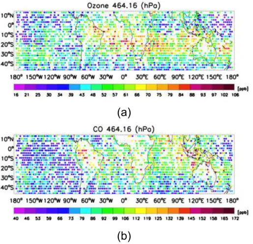
TES observations of ozone and CO are shown from 15 N to 30 S at 464 hPa from 4– 16 November 2004 in Fig. 2. The most notable feature is a band of elevated ozone starting from eastern Brazil through both the Atlantic and Indian Oceans and extending

5

into the Pacific. The highest ozone concentrations are observed both over the tropical Atlantic (>100 ppbv) and over Madagascar. This pervasive zonal ozone distribution has been observed from satellites, in particular from the total ozone mapping spectrometer (TOMS) using a tropospheric ozone residual technique (Fishman and Larsen,1987;

Fishman et al., 1991, 2003). This distribution is due in part to the recirculation of

10

ozone and ozone precursors between South America and sub-equatorial Africa over the Atlantic (Kalnay et al., 1996; Krishnamurti et al., 1996; Thompson et al., 1996;

Sinha et al.,2004).

In addition, a high pressure system centered over Australia, low monthly averaged cloud optical depths from the International Satellite Cloud Climatology Project (ISCCP)

15

(Rossow and Schiffer,1991;Rossow et al.,1993) (available at http://isccp.giss.nasa.

gov/), and relatively high biomass burning (van der Werf et al.,2006) indicate condi-tions favorable to ozone formation. TES observacondi-tions of mid-tropospheric ozone show enhanced values extending northwest of Australia into Indonesia, which have been associated with El Ni ˜no conditions (Thompson et al.,2001;Chandra et al.,2007).

20

TES observations of CO show a plume from South America extending into the west-ern Pacific consistent with previous satellite and aircraft observations (Chatfield et al.,

2002; Edwards et al., 2006). These concentrations in conjunction with MODIS fire-counts are indicative of a continued presence of continental emission sources even as the southern hemisphere transitions to its Austral summer, wet season. Similar to TES

25

ozone, Indonesia-Australia region shows elevated concentrations of TES CO compara-ble to South America and sub-equatorial Africa. In addition, the pervasive high values of CO across the Indian ocean are suggestive of recirculation of emissions between

(11)

ACPD

Full Screen / Esc

EGU

continents, which is consistent with studies from the Southern African Fire-Atmosphere Research Initiative (SAFARI), e.g., (Garstang et al.,1996).

3.1 Comparison of TES ozone to the SHADOZ network

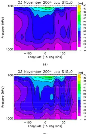
The vertical distribution of ozone over the southern tropics as observed by TES is shown in Fig.3where the TES observations have been averaged in 15◦_{bins between}

5

the equator and 30 S. There were roughly 30 observations for each bin. A pervasive high in ozone is evident across the tropical Atlantic with values up to about 80 ppb from 15 S to the equator. This distribution follows the so-called “wave-one” pattern (

Thomp-son et al.,2000;Logan,1999). From Fig.3a there is a secondary ozone enhancement over Indonesia-northern Australia between 90 E–100 E and 400–500 hPa. A similar

10

picture emerges based on ozone sondes drawn from the SHADOZ network (

Thomp-son et al.,2003a) for November 2004, which is shown in Fig. 4. A total of 30 sondes were used in the average ranging from just one sonde measurement at Java to 6 sonde measurements at Natal. In the tropical Atlantic between 0 and 30 W, Ascencion (8 S, 14.4 W) and Natal (5.8 S, 35.2 W) show middle tropospheric values between 60–

15

80 ppb, consistent with TES observations in Fig.3. At the Java site (7.5 S, 112.6 E), elevated ozone concentrations of 50–70 ppb are observed between 700-400 hPa while TES observations over the same region indicate a similar enhancement. The vertical structure of the ozone over Indonesia is somewhat different than ozone enhancements over the tropical Atlantic and western Indian Ocean suggesting that different processes

20

are controlling ozone formation there.

The vertical distribution of TES ozone from 30 S to 15 S are shown in Fig.3b. Ele-vated ozone stretches from Southern Brazil across the Atlantic and Africa into most of the Indian Ocean. This elevated ozone is pervasive from roughly 500–200 hPa. Com-parison between Pretoria (25.9 S, 28 E) and TES observations show similar values of

25

ozone (80–100 ppb) between 400–200 hPa whereas Reunion Island (21.1 S, 55.5 E) indicates significantly higher ozone above 200 hPa. Similar to the ozone distribution in Fig.2, higher amounts of ozone are seen throughout the troposphere over the Indian

(12)

ACPD

Full Screen / Esc

EGU

Ocean relative to the remote Pacific by roughly 10–20 ppb, consistent with transport of ozone from South America, South Atlantic, and Africa into the Indian Ocean.

4 Signatures of lightning and surface NOx

The concentrations and distribution of NO_x has a significant impact of the distribution of ozone (Jacob et al.,1996). In the southern hemisphere, the primary sources of

sur-5

face NOxare biomass burning, fossil fuel and biofuel combustion (Jaegl ´e et al.,2005).

These emissions can produce ozone near the surface which can in turn be convec-tively lofted into the upper troposphere (Chatfield and Delany,1990). However, NOx

from lightning is directly emitted into the upper troposphere and can play a dominant role in the production of tropical ozone (Pickering et al.,1998;Sauvage et al.,2007;

10

Martin et al.,2007;Boersma et al.,2005). The Lightning Imaging Sensor (LIS) aboard the Tropical Rainfall Measuring Mission (TRMM) estimates lightning flash counts by means of a high speed CCD imaging sensor (3–6 km horizontal resolution) in conjunc-tion with a narrow band (λ=777nm) filter. Lightning flash counts from LIS are shown in Fig.5 for November 2004. For this month, lightning flash counts are densely

dis-15

tributed over Northern Argentina and to a lesser extent southeastern Brazil, throughout tropical Africa and Southern Africa with rates exceeding 150. By comparison, Indone-sia/Northern Australia shows markedly less flash counts with rates generally less than 25. This distribution is consistent with the high pressure system from the NCEP reanal-ysis and the ISCCP cloud optical depth. Consequently, we could expect the regional

20

contribution of ozone from lightning NOx over Indonesia/Australia to be less than the

regional contribution of lightning to South America and Africa.

The distribution of lower tropospheric NO₂ can be investigated from monthly aver-aged tropospheric NO2columns derived from the Ozone Monitoring Instrument (OMI,

(Levelt et al.,2006)), which are shown in Fig.6for November 2004. The columns are

25

calculated using the the retrieval-assimilation algorithm described in (Boersma et al.,

(13)

hori-ACPD

Full Screen / Esc

EGU

zontal resolutions of 25×24 km2 have been gridded onto a 0.5◦×0.5◦ grid. To avoid situations with clouds screening the NO2 underneath, only cloud-free (cloud radiance

fraction <50%) observations were taken. The estimated uncertainty for individual OMI observations is on the order of 30–50% for situations with appreciable NO2 columns

(>1 1015molec/cm2), but it is anticipated that the averaging of large numbers of pixels

5

here reduces the uncertainty of the monthly average to within 5–10%. Given these uncertainties, NO2 tropospheric column values on the order of 8 10

15

molec/cm2 are concentrated south of the mouths of the Amazon in Brazil as well as Northern Aus-tralia. With the exception of Johannesburg region in South Africa where values ap-proach 20 1015molec/cm2 , there are no high concentrations of tropospheric NO2 in

10

sub-equatorial Africa.

5 Comparison of GEOS-Chem to TES estimates of CO and ozone

5.1 Description of GEOS-Chem

The GEOS-Chem global chemistry and transport model was originally described by

(Bey et al., 2001). The simulation conducted for the November 2004 used

GEOS-15

Chem v7.02.04 (http://www-as.harvard.edu:16080/chemistry/trop/index.html) driven by GEOS-4 assimilated meteorological observations from the NASA Global Modeling and Assimilation Office (GMAO). The GEOS-4 observations have a temporal resolution of 6 h (3 h for surface variables and mixing depths), a horizontal resolution of 1◦×1.25◦, and 55 vertical layers. Here we degrade the horizontal resolution to 2◦

×2.5◦ from the

20

surface up to 0.01 hPa. The model includes a complete description of tropospheric O3

-NOx-hydrocarbon chemistry, including sulfate aerosols, black carbon, organic carbon,

sea salt, and dust. Anthropogenic emissions in the model are described in (Duncan

et al.,2007). Extensive evaluations of the GEOS-Chem tropospheric ozone simulations have been conducted by (Wu et al.,2007;Martin et al.,2002;Liu et al.,2006).

(14)

ACPD

Full Screen / Esc

EGU

5.2 Comparison of GEOS-Chem to TES CO over the southern tropics

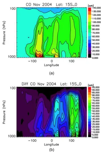
The GEOS-Chem CO zonal distribution from 15◦S to the equator is shown in Fig. 7a. The results are averaged from 4–16 November 2004 in 15◦

×15◦bins. This simulation used climatological biomass burning emissions, which result in elevated values of CO over South America, Africa, and Indonesia/Australia. In the lower and middle

tropo-5

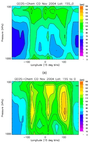
sphere CO over South America dominates the region with values up to 40 ppb higher than Indonesia/Australia. The zonal distribution of TES CO from 15◦S-0 is shown in Fig.8. These retrievals also are averaged in 15◦longitudinal bins with roughly 20–30 observations per bin. For comparison, the GEOS-Chem CO fields were sampled at the coincident TES observation coordinates and the TES observation operator, see

10

Eq. (5), was applied as shown in Fig. 9a. There is significant disagreement both in the magnitude and relative distribution of the GEOS-Chem and TES CO observations with differences up to 40 ppb. TES observations in Fig.8show that CO over Indone-sia/Australia was as high as that over South America.

TES CO observations were used to estimate the CO source emissions over the

15

globe in (Jones et al.,2007). The a priori and a posteriori emissions for South Amer-ica, sub-equatorial AfrAmer-ica, and Australia/Indonesia are listed in Table1. For this time period, the emissions were estimated to be over twice as high as those in the a priori simulation. The GEOS-Chem results at the TES resolution and sampling with the a posteriori emission are shown in Fig.9b. The a posteriori CO distribution from

GEOS-20

Chem between 15◦S and the equator is in remarkably good agreement with the TES observations shown in Fig.8.

The response of GEOS-Chem CO fields to changes in the emissions is shown in Fig. 7b. The maximum increase in CO is over the Indonesia/Australia region is al-most 100 ppb or 85% near the surface and approximately 60 ppb or a 65% increase

25

throughout the free troposphere. Over the Indian Ocean, the CO distribution in GEOS-Chem increased by about 35 ppb over the Indian Ocean and around 45 ppb over sub-equatorial Africa in the 200–400 hPa region. Over South America, the increase is

(15)

ACPD

Full Screen / Esc

EGU

modest – no more than 30 ppb.

5.3 Comparison of GEOS-Chem to TES ozone over the southern tropics

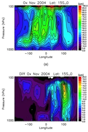
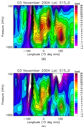
The zonal distribution of ozone from the GEOS-Chem model with a priori emissions is shown in the top panel of Fig.10a from 15◦S-0 averaged in the same manner as CO. GEOS-Chem follows the familiar “wave-one” pattern (Thompson et al., 2003b) with

5

enhanced values of ozone across the tropical Atlantic. However, there is a modest secondary maximum in ozone over Indonesia/Australia relative to the Pacific. This en-hancement is also observed in Fig.11a where the TES observation operator has been applied to the GEOS-Chem fields. In both cases, the ozone amounts are less than those observed by TES in Fig.3over both the tropical Atlantic and Indonesia/Australia.

10

The ozone distribution from GEOS-Chem was also calculated based on the revised emissions where the NO_x emissions were scaled with the CO a posteriori emission estimates. The GEOS-Chem fields with the a posteriori emissions sampled along the TES observations are shown in Fig.11b. There is an increase in upper tropospheric ozone at 200 hPa over the tropical Atlantic and at 280 hPa over sub-equatorial Africa.

15

In addition, an overall increase of about 10 ppb throughout the troposphere can be seen over Indonesia/Australia. Use of the a posteriori emissions improves agreement between the model and TES ozone, but significant discrepancies remain.

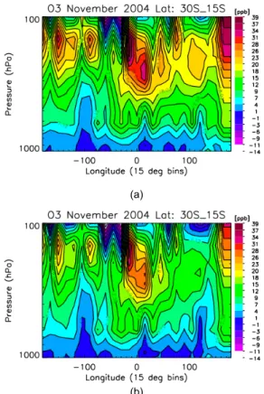
The difference between the TES observations of ozone and GEOS-Chem with a pri-ori (top panels) and a posteripri-ori (bottom panels) emissions are shown in Fig.12 for

20

15 S to the equator and Fig.13 for 30 S to 15 S. The top panels show the largest dif-ferences in ozone are centered over the Atlantic and Indonesia. With the a posteriori emissions, the bottom panels show an overall decrease in ozone differences that is fairly uniform zonally. Over the tropical Atlantic, the difference between GEOS-Chem and TES are reduced by roughly 5 ppb from 30 S-0. The reduction over the

Indone-25

sia/Australia region in the mid-troposphere is more substantial: up to 10 ppb. On the other hand, the upper tropospheric ozone differences at 100 E and 100 W from 15 S-0 increased with the a posteriori emissions. With those exceptions, TES observations

(16)

ACPD

Full Screen / Esc

EGU

are higher everywhere relative to GEOS-Chem.

In contrast to the a posteriori CO comparisons with TES observations (Fig.9), there remains significant residual differences in ozone. This residual indicates that assump-tions used in the emissions are incorrect, e.g., the relative distribution of CO to NO_x, pathways relating those emissions to ozone formation are deficient, or background

5

processes have not be properly described. Over the Atlantic, the residual differences and their spatial structure can be attributed in part to ozone generated from lightning NOx. In (Sauvage et al., 2007), increasing the intra-cloud to ground-to-cloud flash

ratio to 0.75 for lightning NOx formation considerably improved agreement between

GEOS-Chem and SHADOZ network ozone for the September-October-November

sea-10

son (although this increase reduced agreement in other seasons). The peak changes in ozone to this ratio were centered between 500–300hPa over the Ascension Islands and increased ozone there by 10–20 ppb, which is consistent with the residual differ-ence in Fig.12b. In addition, there is a residual difference over Indonesia/Australia at 600 hPa of up to 15 ppb that can not be explained by surface emissions. This difference

15

may reflect deficiencies in sources of NOx from regional lightning, vertical mixing, or

assumed composition of the emission sources.

5.4 Response of GEOS-Chem to changes in ozone and NOxdistribution from a

pos-teriori emission estimates

We can use the emission estimates to investigate chemical mechanisms linking those

20

emissions to the tropical ozone distribution and to interpret the residual differences be-tween TES and GEOS-Chem ozone distributions. The averaged difference bebe-tween GEOS-Chem ozone fields with a priori and a posteriori emissions are shown in Fig.10. The largest differences in ozone from the change in emissions are over the Indone-sia/Australia regions where ozone increases by up to 16 ppb in the upper troposphere

25

centered around 150 hPa. It is in this upper tropospheric region, as shown in Fig.12b, that GEOS-Chem ozone is greater than the TES observations by up to 15%. The amount of ozone produced, however, will be sensitive to the chemical composition of

(17)

ACPD

Full Screen / Esc

EGU

the lofted emissions. Consequently, one interpretation is that the overestimate is due to uniform scaling of all combustion sources.

The ozone response to the emission changes over sub-equatorial Africa is approx-imately 8 ppb near the surface and around 200 ppb. Over South America, there were few changes in the ozone distribution, consistent with a modest increase in emission

5

strengths. Curiously, there was a significant increase in ozone in the remote Pacific centered around 150 S in the upper troposphere (>15%).

The principle chemical mechanism for the ozone response in the free troposphere to changes in surface emissions is the ambient NOxdistribution. CO is assumed to be

a tracer of emissions generally and consequently all the emissions, including NO_x, are

10

scaled along with the CO emissions derived from the inverse analysis. However, the NOx zonal distribution has a different response to the scaled emissions than the CO

distribution. The NOx distribution based on the GEOS-Chem a priori emissions and

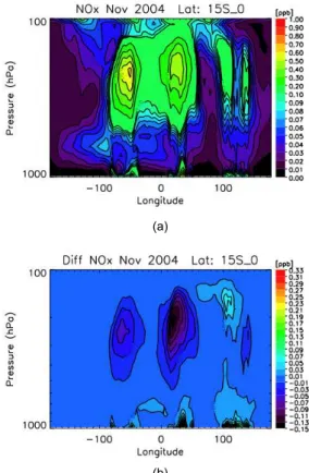
the change in mean zonal NO_x from the a posteriori emissions are shown in Fig.14. The a priori NOxfields are highest over South America where the values are up to 6–7

15

times higher than over Indonesia/Australia and up to twice as high as sub-equatorial Africa. The concentrations of NO_xin the free troposphere are due primarily to lightning sources (Pickering et al., 1998; Folkins et al., 2006), with the South American and sub-equatorial African regions exhibiting a much larger source of NOx from lightning

than the Indonesian/Australian regions. Qualitatively, this distribution is consistent with

20

the LIS observations in Fig. 5. Associated with the higher concentrations of NOx,

the model simulation with the a priori emissions also produces more ozone (Fig. 10) over South America and sub-equatorial Africa than over Indonesia/Australia. The low ozone abundance over Indonesia/Australia, however, also reflects convective transport of ozone-poor marine air to the upper troposphere (Lelieveld et al.,2001). Enhanced

25

ozone over South America and sub-equatorial Africa results in greater concentrations of OH (by more than a factor of 2) over these regions, which together with the higher NOx levels leads to significantly more HNO3 (by almost an order of magnitude) over

(18)

ACPD

Full Screen / Esc

EGU

The greatest increase in free tropospheric NO_x(100 ppt) to the a posteriori emissions is centered over the Java Sea (115 E) at 150 hPa just to the east of the high NOx

concentrations over Sumatra (105 E). Conversely the greatest decrease (>120 ppt) in free tropospheric NO_xis located over the western coast of Africa. In addition, there is a significant decrease over South America (>55 ppt) centered at 250 hPa. The response

5

of free tropospheric NOx to increases in the surface emissions, which include surface

NO_x, is a non-linear function of both the ambient amounts of ozone, NO_x, and OH along with the chemical composition of lofted emissions. Over Indonesia/Australia the dominant sink for NOx is formation of peroxyacetylnitrate (PAN), whereas over South

America and Africa NO_x is lost through formation of PAN and HNO₃(due to the higher

10

levels OH in these regions). In addition, the NO/NO₂ratio is lower over South America and Africa because of the higher abundances of ozone in these regions. This enhances the conversion of NOx to PAN and HNO3.

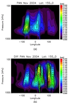
Another important difference between the three tropical continental regions is the distribution of organics such as acetaldehyde, acetone, and formaldehyde in the free

15

troposphere. Acetaldehyde, for example, is oxidized by reaction with OH to produce peroxyacetyl radicals (CH₃C(O)OO) that in turn react with NO₂to form PAN. The mean difference in PAN concentrations between the simulations with the a priori and a poste-riori emissions is shown in Fig.15. The response of upper tropospheric PAN to surface emission changes above Africa is over 150 ppt, which is roughly 50% greater than

20

over Indonesia/Australia. Tropospheric PAN also increased over South America with changes up to 100 ppt. We can conclude that, for this time period, increases in surface emissions over South America and sub-equatorial Africa preferentially lead to the for-mation of PAN at the expense of NOxand consequently mute the production of ozone.

On the other hand, increased surface emissions in Indonesia/Australia, while leading

25

to enhanced PAN, do not lead to a reduction of NO_x due to the overall lower back-ground concentrations of NOx, OH, and carbonyl compounds. Consequently, ozone

production is regionally enhanced. The different responses to increased emissions over these three regions illustrate the importance of both background meteorological

(19)

ACPD

Full Screen / Esc

EGU

conditions and the particular chemical composition of the emissions in linking ozone production to surface emissions. These responses must be characterized in order to reduce uncertainty both in present day and future changes in ozone (Horowitz,2006).

6 Conclusions

We have investigated the processes controlling the zonal distribution of tropical

tropo-5

spheric ozone with a focus on the sensitivity of that distribution to changes in surface emissions between South America, sub-equatorial Africa, and Indonesia/Australia for November, 2004.

Against the backdrop of the “wave-one” pattern of elevated ozone in the tropical Atlantic, TES ozone profiles also indicate enhanced values over Indonesia/Australia

10

with volume mixing ratios up to 70 ppb at 600 hPa. This enhancement is consistent with a SHADOZ sonde observation over Java. Co-located CO profiles from TES and NO2

columns from OMI indicate concentrations over Indonesia/Australia are comparable to those over South America and Africa.

From this observational context, we assessed the contribution of surface emissions

15

to tropical ozone using GEOS-Chem simulations with a posteriori emissions derived from a linear inverse model, which was based on TES and MOPITT CO developed in (Jones et al., 2007). Based on over a factor of 2 increase in surface emissions in sub-equatorial Africa and Indonesia/Australia, the overall difference between TES and GEOS-Chem ozone was reduced throughout the troposphere between 30 S-0.

20

Over Africa and Indonesia/Australia the discrepancies between GEOS-Chem and TES decreased by roughly 10 ppb.

While there was overall improvement between TES ozone observations and GEOS-Chem, there remained substantial disagreements. Maximum residual differences of approximately 18 ppb are seen between 15 S-0 and 30 ppb between 30 S–15 S. In the

25

upper troposphere over the Eastern Indian Ocean and parts of the Western Pacific, GEOS-Chem overestimated the ozone distributions by 5 ppb.

(20)

ACPD

Full Screen / Esc

EGU

The residual differences in ozone of 10–20 ppb in the mid-troposphere over the trop-ical Atlantic are consistent with the differences found in (Sauvage et al.,2007) associ-ated with underestimates of lightning NOxformation in GEOS-Chem for the

September-October-November season. In addition, there is a residual difference over Indone-sia/Australia at 600 hPa of up to 15 ppb that can not be explained by surface emissions.

5

We investigated these residual differences further by examining the spatial patterns in GEOS-Chem estimates of ozone, CO, and NOx from changes between the a

pri-ori and a posteripri-ori surface emissions. The greatest change to the free tropospheric ozone distribution from 15 S-0 was over Indonesia (<16 ppb) at 175 hPa, consistent with maximum positive changes in NOx (<100 ppt) and CO (<70 ppb). Consequently,

10

free tropospheric ozone over Indonesia/Australia is sensitive to changes in regional surface emissions and these emissions make a significant contribution to the regional ozone budget.

On the other hand, the free tropospheric NO_x distribution declined over Africa and South America with losses exceeding 150 ppt. We examined the PAN response as a

15

possible loss mechanism for the NOx. Maximum increases in PAN, which reached over

150 ppt, corresponded to the maximum decreases in the NO_x distribution. Therefore, conversion of NOx to PAN can partially explain the decreases in NOx in response to

increases in surface emission over South America and Africa. If this mechanism is cor-rect, then the sensitivity of the tropical Atlantic ozone to changes in surface emissions

20

of NOx is low because of the large ambient distribution of ozone and NOx from

light-ning. However, the enhanced PAN could lead to additional ozone formation downwind through conversion of PAN back to NO_x (Staudt et al.,2003).

Based on scenarios discussed in the IPCC-4, the tropical latitudes are particularly sensitive to climate change in terms of precipitation and land-use(Solomon et al.,

25

2007). Based on our results, the emissions from Indonesia/Australian are an important contributor to the zonal tropical ozone distribution both in terms of the ozone produced and in the sensitivity of ozone to changes in those emissions. Given the complex feedbacks between land-use, biomass burning, biofuel production, plant productivity,

(21)

ACPD

Full Screen / Esc

EGU

and CO₂ uptake and emission, (Levine,1999;Sitch et al.,2007;Lohman et al.,2007;

Forster et al.,2007), quantifying the present and future impact of surface emissions to tropical ozone will be critical for understanding chemistry-climate coupling.

Acknowledgements. This work was performed, in part, at the Jet Propulsion Laboratory,

Cali-fornia Institute of Technology, under a contract with the National Aeronautics and Space

Admin-5

istration (NASA). J. Logan was funded by a grant from NASA to Harvard University. D. Jones was supported by funding from the Natural Sciences and Engineering Research Council of Canada. We also thank the SHADOZ program for making the sonde data accessible.

References

Arellano, A. F., Kasibhatla, P. S., Giglio, L., van der Werf, G. R., Randerson, J. T., and Collatz,

10

G. J.: Time-dependent inversion estimates of global biomass-burning CO emissions using Measurement of Pollution in the Troposphere (MOPITT) measurements, J. Geophys. Res, 111, D09303, doi:10.1029/2005JD006613, 2006. 1507

Beer, R. and Glavich, T.: Remote Sensing of the Troposphere by Infrared Emissions Spec-troscopy, Appl. Optics, 1129, 42–51, 1989. 1509

15

Bey, I., Jacob, D. J., Yantosca, R. M., Logan, J. A., Field, B. D., Fiore, A. M., Li, Q., Liu, H. Y., Mickley, L. J., and Schultz, M. G.: Global modeling of tropospheric chemistry with assimilated meteorology: Model description and evaluation, J. Geophys. Res., 106(D19), 23 073–23 095, 2001. 1516

Boersma, K., Eskes, H. J., Veefkind, J. P., Brinskma, E. J., van der A, R. J., Sneep, M., van den

20

Oord, G. H. J., Levelt, P. F., Stammes, P., Gleason, J. F., and Bucsela, E. J.: Near-real time retrieval of tropospheric NO₂from OMI, Atmos. Chem. Phys., 7, 2103–2118, 2007,

http://www.atmos-chem-phys.net/7/2103/2007/. 1515

Boersma, K. F., Eskes, H. J., and Brinksma, E. J.: Error analysis for tropospheric NO₂retrieval from space, J. Geophys. Res.-Atmospheres, 109, D04311, doi:10.1029/2003JD003962,

25

2004. 1515

Boersma, K. F., Eskes, H. J., Meijer, E. W., and Kelder, H. M.: Estimates of lightning NOx production from GOME satellite observations, Atmos. Chem. Phys., 5, 2311–2331, 2005,

(22)

ACPD

Full Screen / Esc

EGU

Bowman, K., Worden, J., Steck, T., Worden, H., Clough, S., and Rodgers, C.: Capturing time and vertical variability of tropospheric ozone: A study using TES nadir retrievals, J. Geophys. Res., 107, 4723, doi:10.1029/2002JD002150, 2002. 1510

Bowman, K. W., Rodgers, C. D., Kulawik, S. S., Worden, J., Sarkissian, E., Osterman, G., Steck, T., Lou, M., Eldering, A., Shephard, M., Worden, H., Lampel, M., Clough, S., Brown,

5

P., Rinsland, C., Gunson, M., and Beer, R.: Tropospheric Emission Spectrometer: Retrieval Method and Error Analysis, IEEE T. Geosci. Remote, 44, doi:10.1109/TGRS.2006.871234, 2006. 1510

Chandra, S., Ziemke, J. R., Schoeberl, M. R., Froidevaux, L., Read, W. G., Levelt, P. F., and Bhartia, P. K.: Effects of the 2004 El Ni ˜no on tropospheric ozone and water vapor, Geophys.

10

Res. Lett., 34, L06802, doi:10.1029/2006GL028779, 2007. 1513

Chatfield, R. B. and Delany, A.: Convection links biomass burning to increased tropical ozone: However, models will tend to overpredict O₃, J. Geophys. Res.-Atmospheres, 95(D11), 18 473–18 488, 1990. 1515

Chatfield, R. B., Guo, Z., Sachse, G. W., Blake, D. R., and Blake, N. J.: The subtropical global

15

plume in the Pacific Exploratory Mission-Tropics A (PEM-Tropics A), PEM-Tropics B, and the Global Atmospheric Sampling Program (GASP): How tropical emissions affect the remote Pacific, J. Geophys. Res., 107(D16), doi:10.1029/2001JD000497, 2002. 1513

Duncan, B. N., Bey, I., Chin, M., Mickley, L. J., Fairlie, T. D., Martin, R. V., and Matsueda, H.: Indonesian wildfires of 1997: Impact on tropospheric chemistry, J. Geophys. Res., 108,

20

4458, doi:10.1029/2002JD003195, 2003a. 1507

Duncan, B. N., Martin, R. V., Staudt, A. C., Yevich, R., and Logan, J. A.: Interannual and seasonal variability of biomass burning emissions constrained by satellite observations, J. Geophys. Res., 108, 4100, doi:10.1029/2002JD002378, 2003b.1507

Duncan, B. N., Logan, J. A., Bey, I., Megretskaia, I. A., and Yantosca, R. M.: The global

25

budget of CO, 1988-1997: source estimates and validation with a global model, J. Geophys. Res.,112, D22301, doi:10.1029/2007JD008459, 2007. 1516

Edwards, D. P., Emmons, L. K., Gille, J. C., Chu, A., Atti ´e, J.-L., Giglio, L., Wood, S. W., Haywood, J., Deeter, M. N., Massie, S. T., Ziskin, D. C., and Drummond, J. R.: Satellite-observed pollution from Southern Hemisphere biomass burning, J. Geophys. Res., D14312,

30

doi:10.1029/2005JD006655, 2006. 1513

Fishman, J. and Larsen, J. C.: Distribution of total ozone and stratospheric ozone in the tropics: Implications for the distribution of tropospheric ozone, J. Geophys. Res., 92, 6627–6634,

(23)

ACPD

Full Screen / Esc

EGU

1987. 1507,1513

Fishman, J., Ramanathan, V., Crutzen, P. J., and Liu, S. C.: Tropospheric ozone and climate, Nature, 282, 818–820, doi:10.1038/282818a0, 1979. 1507

Fishman, J., Fakhruzzaman, K., Cros, B., and Nganga, D.: Identification of Widespread Pollu-tion in the Southern Hemisphere deduced from satelite analyses, Science, 252, 1693–1696,

5

1991. 1507,1508,1513

Fishman, J., Wozniak, A. E., and Creilson, J. K.: Global distribution of tropospheric ozone from satellite measurements using the empirically corrected tropospheric ozone residual tech-nique: Identification of the regional aspects of air pollution, Atmos. Chem. Phys., 3, 2003.

1513 10

Folkins, I., Bernath, P., Boone, C., Donner, L. J., Eldering, A., Lesins, G., Martin, R. V., Sinnhu-ber, B.-M., and Walker, K.: Testing convective parameterizations with tropical measurements of HNO₃, CO, H₂O, and O₃: Implications for the water vapor budget, J. Geophys. Res., 111, D23304, doi:10.1029/2006JD007325, 2006. 1520

Forster, P., Ramaswamy, V., Artaxo, P., Berntsen, T., Betts, R., Fahey, D., Haywood, J., Lean, J.,

15

Lowe, D., Myhre, G., Nganga, J., Prinn, R., Raga, G., Schulz, M., and Dorland, R. V.: Climate Change 2007: The Physical Science Basis. Contribution of Working Group I to the Fourth Assessment Report of the Intergovernmental Panel on Climate Change, chap. Changes in Atmospheric Constituents and in Radiative Forcing, 131–217, Cambridge University Press, 2007. 1524

20

Garstang, M., Tyson, P. D., Swap, R., Edwards, M., Kallberg, P., and Lindesay, J. A.: Horizontal and vertical transport of air over southern Africa, J. Geophys. Res., 101, 23 721–23 736, 1996. 1514

Hauglustaine, D., Emmons, L., Newchurch, M., Brasseur, G., Takao, T., Matsubara, K., John-son, J., Ridley, B., Stith, J., and Dye, J.: On the Role of Lightning NOx in the Formation of

25

Tropospheric Ozone Plumes: A Global Model Perspective, J. Atmos. Chem., 38, 277–294, 2001. 1508

Horowitz, L.: Past, present, and future concentrations of tropospheric ozone and aerosols: Methodology, ozone evaluation, and sensitivity to aerosol wet removal, J. Geophys. Res., 111, D22211, doi:10.1029/2005JD006937, 2006. 1522

30

Jacob, D., Heikes, B. G., Fan, S.-M., Logan, J. A., Mauzerall, D. L., Bradshaw, J. D., Singh, H. B., Gregory, G. L., Talbot, R. W., Blake, D. R., and Sachse, G. W.: Origin of ozone and NOx in the tropical troposphere: A photochemical analysis of aircraft observations over the

(24)

ACPD

Full Screen / Esc

EGU

South Atlantic basin, J. Geophys. Res., 101(D19), 24 235–24 250, doi:10.1029/96JD00336, 1996. 1507,1515

Jacob, D. J.: Introduction to Atmospheric Chemistry, Princeton University Press, New Jersey, 1999. 1507

Jaegl ´e, L., Steinberger, L., Martin, R. V., and Chance, K.: Global partitioning of NOx sources

5

using satellite observations: Relative roles of fossil fuel combustion, biomass burning and soil emissions, Faraday Discuss., 130, 407–423, doi:10.1039/b502128f, 2005. 1515

Jenkins, G. S. and Ryu, J.-H.: Space-borne observations link the tropical atlantic ozone maximum and paradox to lightning, Atmos. Chem. Phys., 4, 361–375, available at:

http://www.atmos-chem-phys.net/4/361/2004/acp-4-361-2004.pdf, 2004a. 1507 10

Jenkins, G. S. and Ryu, J.-H.: Linking horizontal and vertical transports of biomass fire emis-sions to the tropical Atlantic ozone paradox during the Northern Hemisphere winter season: climatology, Atmos. Chem. Phys., 4, 449–469, 2004b. 1507

Jones, D. B. A., Bowman, K. W., Palmer, P. I., Worden, J. R., Jacob, D. J., Hoffman, R. N., Bey, I., and Yantosca, R. M.: Potential of observations from the Tropospheric Emission

Spec-15

trometer to constrain continental sources of carbon monoxide, J. Geophys. Res., 108, 4789, doi:10.1029/2003JD003702, 2003. 1512

Jones, D. B. A., Bowman, K. W., Logan, J. A., and et al: Integrated analysis of carbon monoxide emissions from biomass burning using data from the TES and MOPITT satellite instruments, Atmos. Chem. Phys. Discuss., 2007. 1506,1508,1517,1522,1533

20

Jourdain, L., Worden, H. M., Worden, J. R., Bowman, K., Li, Q., Eldering, A., Kulawik, S. S., Osterman, G., Boersma, K. F., Fisher, B., Rinsland, C. P., Beer, R., and Gun-son, M.: Tropospheric vertical distribution of tropical Atlantic ozone observed by TES dur-ing the northern African biomass burndur-ing season, Geophys. Res. Lett., 34, L04810, doi: 10.1029/2006GL028284, 2007. 1507

25

Kalnay, E., Kanamitsu, M., Kistler, R., Collins, W., Deaven, D., Gandin, L., Iredell, M., Saha, S., White, G., Woollen, J., Zhu, Y., Chellah, M., Ebisuzaki, W., Higgins, W., Janowiak, J., Mo, K. C., Ropelewski, C., Wang, J., Leetma, A., Reynolds, R., Jenne, R., and Joseph, D.: The NCEP/NCAR 40-Year and Reanalysis Project, B. Am. Meteorol. Soc., 77, 437–471, 1996.

1513 30

Kiehl, J. T., Schneider, T. L., Portmann, R. W., and Solomon, S.: Climate forcing due to tropo-spheric and stratotropo-spheric ozone, J. Geophys. Res., 104, 31 239–31 254, 1999. 1507

(25)

Ja-ACPD

Full Screen / Esc

EGU

cob, D. J., and Logan, J.: Passive tracer transport relevant to the TRACE A experiment, J. Geophys. Res., 101, 23 889–23 908, doi:10.1029/95JD02419, 1996.1513

Lacis, A., Wuebbles, D. J., and Logan, J. A.: Radiative forcing of climate by changes in the vertical distribution of ozone, J. Geophys. Res., 95(D7), 9971–9981, 1990. 1507

Lelieveld, J., Crutzen, P. J., Ramanathan, V., Andreae, M. O., Brenninkmeijer, C. A. M.,

Cam-5

pos, T., Cass, G. R., Dickerson, R. R., Fischer, H., de Gouw, J. A., Hansel, A., Jefferson, A., Kley, D., de Laat, A. T. J., Lal, S., Lawrence, M. G., Lobert, J. M., Mayol-Bracero, O. L., Mitra, A. P., Novakov, T., Oltmans, S. J., Prather, K. A., Reiner, T., Rodhe, H., Scheeren, H. A., Sikka, D., and Williams, J.: The Indian Ocean Experiment: Widespread Air Pollution from South and Southeast Asia, Science, 291, 1031–1036, doi:10.1126/science.1057103, 2001.

10

1520

Levelt, P. F., Gijsbertus, van den Oord, H. J., Dobber, M. R., M ¨alkki, A., Visser, H., de Vries, J., Stammes, P., Lundell, J. O. V., and Saari, H.: The Ozone Monitoring Instrument, IEEE T. Geosci. Remote , 44, 1093–1101, 2006. 1515

Levine, J. S.: The 1997 fires in Kalimantan and Sumatra, Indonesia: Gaseous and particulate

15

emissions, Geophys. Res. Lett., 26(7), 815–818, 1999. 1524

Li, Q., Jacob, D. J., Bey, I., Palmer, P. I., Duncan, B. N., Field, B. D., Martin, R. V., Fiore, A. M., Yantosca, R. M., Parrish, D. D., Simmonds, P. G., and Oltmans, S. J.: Transatlantic transport of pollution and its effects on surface ozone in Europe and North America, J. Geophys. Res., 107, doi:10.1029/2001JD001422, 2002.1507

20

Liu, X., Chance, K., Sioris, C. E., Kurosu, T. P., Spurr, R. J. D., Martin, R. V., Fu, T.-M., Logan, J. A., Jacob, D. J., Palmer, P. I., Newchurch, M. J., Megretskaia, I. A., and Chatfield, R. B.: First directly retrieved global distribution of tropospheric column ozone from GOME: Com-parison with the GEOS-CHEM model, J. Geophys. Res., 111, doi:10.1029/2005JD006564, 2006. 1516

25

Logan, J.: An Analysis of ozonesonde data for the troposphere: Recommendations for testing 3-D models and development of a gridded climatology for tropospheric ozone, J. Geophys. Res., 104, 16 115–16 149, 1999. 1514

Logan, J. A. and Kirchoff, V.: Seasonal variations of tropospheric ozone at Natal, Brazil, J. Geophys. Res., 91, 7875–7881, 1986.1508

30

Lohman, D. J., Bickford, D., and Sodhi, N. S.: The Burning Issue, Science, 316, 2007.1524

Luo, M., Rinsland, C., Fisher, B., Sachse, G., Diskin, G., Logan, J., Worden, H., Kulawik, S., Osterman, G., Eldering, A., Herman, R., and Shephard, M.: TES carbon monoxide validation

(26)

ACPD

Full Screen / Esc

EGU

with DACOM aircraft measurements during INTEX-B 2006, J. Geophys. Res., 112, D24S48, doi:10.1029/2007JD008803, 2007a.1510

Luo, M., Rinsland, C. P., Rodgers, C. D., Logan, J. A., Worden, H., Kulawik, S., Eldering, A., Goldman, A., Shephard, M. W., Gunson, M., and Lampel, M.: Comparison of carbon monoxide measurements by TES and MOPITT – the influence of a priori data and instrument

5

characteristics on nadir atmospheric species retrievals, J. Geophys. Res., D09303, doi:10. 1029/2006JD007663, 2007b. 1510

Marenco, A., Thouret, V., N ´ed ´elec, P., Athierlec, G., Smit, H., Helten, M., Kley, D., Karcher, F., Simon, P., Law, K., Pyle, J., Poschmann, G., Wrede, R. V., Hume, C., and Cook, T.: Measure-ment of ozone and water vapor by Airbus in-service aircraft: The MOZAIC airborne program,

10

An overview, J. Geophys. Res., 103, 25 631–25 642, doi:10.1029/98JD00977, 1998. 1508

Martin, R., Jacob, D. J., Logan, J. A., Ziemke, J. M., and Washington, R.: Detection of a lightning influence on tropical tropospheric ozone, Geophys. Res. Lett., 27, 1639–1642, 2000. 1507

Martin, R. V., Jacob, D. J., Logan, J. A., Bey, I., Yantosca, R. M., Staudt, A. C., Li, Q., Fiore, A. M., Duncan, B. N., and Liu, H.: Interpretation of TOMS observations of tropical

tropo-15

spheric ozone with a global model and in situ observations, J. Geophys. Res., 107, 4351, doi:10.1029/2001JD001480, 2002.1507,1508,1516

Martin, R. V., Sauvage, B., Folkins, I., Sioris, C. E., Boone, C., Bernath, P., and Ziemke, J.: Space-based constraints on the production of nitric oxide by lightning, J. Geophys. Res., 112, D09309, doi:10.1029/2006JD007831, 2007. 1515

20

Naik, V., Mauzerall, D., Horowitz, L., Schwarzkopf, M. D., Ramaswamy, V., and Oppenheimer, M.: Net radiative forcing due to changes in regional emissions of tropospheric ozone precur-sors, J. Geophys. Res., 110, D24306, doi:10.1029/2005JD005908, 2005. 1507

Nassar, R., Logan, J., Worden, H., Megretskaia, I. A., Bowman, K., Osterman, G., Thompson, A. M., Tarasick, D. W., Austin, S., Claude, H., Dubey, M. K., Hocking, W. K., Johnson, B. J.,

25

Joseph, E., Merrill, J., Morris, G. A., Newchurch, M., Oltmans, S. J., Posny, F., and Schmidlin, F.: Validation of Tropospheric Emission Spectrometer (TES) Nadir Ozone Profiles Using Ozonesonde Measurements, J. Geophys. Res, in press, 2007.1509

Oltmans, S. J., Johnson, B. J., J. M. Harris, H. V., Thompson, A. M., Koshy, K., Simon, P., Bendura, R. J., Logan, J. A., Hasebe, F., Shiotani, M., Kirchhoff, V. W. J. H., Maata, M.,

30

Sami, G., Samad, A., Tabuadravu, J., Enriquez, H., Agama, M., Cornejo, J., and Paredes, F.: Ozone in the Pacific tropical troposphere from ozonesonde observations, J. Geophys. Res., 106, 32 503–32 526, 2001. 1508

(27)

ACPD

Full Screen / Esc

EGU

Osterman and et al: Tropospheric Emission Spectrometer TES L2 Data User’s Guide, Tech. Rep. V3.00, Jet Propulsion Laboratory, California Institute of Technology, Pasadena, CA, 2007. 1509,1511

Osterman, G., Kulawik, S., Worden, H., Richards, N., Fisher, B., Eldering, A., Shephard, M., Froidevaux, L., Labow, G., Luo, M., Herman, R., and Bowman, K.: Validation of Tropospheric

5

Emission Spectrometer (TES) Measurements of the Total, Stratospheric and Tropospheric Column Abundance of Ozone, J. Geophys. Res., in press, 2007. 1510

Pickering, K., Wang, Y., Tao, W.-K., Price, C., and M ¨uller, J.-F.: Vertical distributions of light-ning NOx for use in regional and global chemical transport models, J. Geophys. Res., 103, 31 203–31 216, 1998. 1507,1515,1520

10

Portmann, R. W., Solomon, S., Fishman, J., Olson, J., Kiehl, J., and Briegleb, B.: Radiative forc-ing of the Earth’s climate system due to tropical tropospheric ozone production, J. Geophys. Res., 102(D8), 9409–9417, 1997.1507

Richards, N. A. D., Osterman, G. B., Browell, E. V., Avery, M., and Li, Q.: Validation of Tro-pospheric Emission Spectrometer (TES) Ozone Profiles with Aircraft Observations During

15

INTEX-B, J. Geophys. Res., in press, 2007.1510

Rodgers, C.: Inverse Methods for Atmospheric Sounding: Theory and Practise, World Scien-tific, London, 2000. 1511

Rossow, W. and Schiffer, R.: ISCCP Cloud Data Products, B. Am. Meteorol. Soc., 72, 2–20, 1991. 1513

20

Rossow, W., Walker, A., and Garder, L.: Comparison of ISCCP and Other Cloud Amounts, J. Climate, 6, 2394–2418, 1993. 1513

Sauvage, B., Martin, R. V., van Donkelaar, A., Liu, X., Chance, K., Jaegl ´e, L., Palmer, P. I., Wu, S., and Fu, T.-M.: Remote sensed and in situ constraints on processes affecting tropical tropospheric ozone, Atmos. Chem. Phys., 7, 815–838, 2007,

25

http://www.atmos-chem-phys.net/7/815/2007/. 1508,1515,1519,1523

Sinha, P., Jaegl ´e, L., Hobbs, P. V., and Liang, Q.: Transport of biomass burning emissions from southern Africa, J. Geophys. Res., 109, D20204, doi:10.1029/2004JD005044, 2004. 1513

Sitch, S., Cox, P. M., Collins, W. J., and Huntingford, C.: Indirect radiative forcing of climate change through ozone effects on the land-carbon sink, Nature, doi:10.1038/nature06059,

30

2007. 1524

Solomon, S., Qin, D., Manning, M., Alley, R., Berntsen, T., Bindoff, N., Chen, Z., Chidthaisong, A., Gregory, J., Hegerl, G., Heimann, M., Hewitson, B., Hoskins, B., Joos, F., Jouzel, J.,

(28)

ACPD

Full Screen / Esc

EGU

Kattsov, V., Lohmann, U., Matsuno, T., Molina, M., Nicholls, N., Overpeck, J., Raga, G., Ra-maswamy, V., Ren, J., Rusticucci, M., Somerville, R., Stocker, T., Whetton, P., Wood, R., and Wratt, D.: Climate Change 2007: The Physical Science Basis. Contribution of Working Group I to the Fourth Assessment Report of the Intergovernmental Panel on Climate Change, chap. Technical Summary, 20–90, Cambridge University Press, 2007. 1523

5

Staudt, A. C., Jacob, D. J., Ravetta, F., Logan, J. A., Bachiochi, D., Krishnamurti, T. N., Sand-holm, S., Ridley, B., Singh, H. B., and Talbot, B.: Sources and chemistry of nitrogen oxides over the tropical Pacific, J. Geophys. Res., 108, 8239, doi:10.1029/2002JD002139, 2003.

1523

Thompson, A., Doddridge, B. G., Witte, J. C., Hudson, R. D., Luke, W. T., Johnson, J. E.,

10

Johnson, B. J., Oltmans, S. J., and Weller, R.: A tropical Atlantic ozone paradox: Shipboard and satellite views of a tropospheric ozone maximum and wave-one in January – February 1999, Geophys. Res. Lett., 27, 3317–3320, 2000. 1508,1514

Thompson, A. M., Diab, R. D., Bodeker, G. E., Zunckel, M., Coetzee, G. J. R., Archer, C. B., McNamara, D. P., Pickering, K. E., Combrink, J., Fishman, J., and Nganga, D.: Ozone over

15

southern Africa during SAFARI-92/TRACE A, J. Geophys. Res., 101, 23 793–23 708, 1996.

1513

Thompson, A. M., Witte, J. C., Hudson, R. D., Guo, H., Herman, J. R., and Fujiwara, M.: Tropical Tropospheric Ozone and Biomass Burning, Science, 291, 128–2132, 2001. 1508,1513

Thompson, A. M., Witte, J. C., McPeters, R. D., Oltmans, S. J., Schmidlin, F. J., Logan, J. A.,

20

Fujiwara, M., Volker, Kirchhoff, W. J. H., Posny, F., Coetzee, G. J. R., Hoegger, B., Kawakami, S., Ogawa, T., Johnson, B. J., V ¨omel, H., and Labow, G.: Southern Hemisphere Additional Ozonesondes (SHADOZ) 1998–2000 tropical ozone climatology 1. Comparison with Total Ozone Mapping Spectrometer (TOMS) and ground-based measurements, J. Geophys. Res., 108, 8238, doi:10.1029/2001JD000967, 2003a.1514

25

Thompson, A. M., Witte, J. C., Oltmans, S. J., Schmidlin, F. J., Logan, J. A., Fujiwara, M., Kirch-hoff, V. W. J. H., Posny, F., Coetzee, G. J. R., Hoegger, B., Kawakami, S., Ogawa, T., Fortuin, J. P. F., and Kelder, H. M.: Southern Hemisphere Additional Ozonesondes (SHADOZ) 1998 – 2000 tropical ozone climatology 2. Tropospheric variability and the zonal wave-one, J. Geo-phys. Res., 108, 8241, doi:10.1029/2002JD002241, 2003b.1508,1518

30

van der Werf, G. R., Randerson, J. T., Giglio, L., Collatz, G. J., Kasibhatla, P. S., and A. F. Arel-lano, J.: Interannual variability in global biomass burning emissions from 1997 to 2004, At-mos. Chem. Phys., 6, 3423–3441, available at: www.atmos-chem-phys.net/6/3423/2006/,

(29)

ACPD

Full Screen / Esc

EGU

2006. 1513

Worden, H. M., Logan, J. A., Worden, J. R., Beer, R., Bowman, K., Clough, S. A., Eldering, A., Fisher, B. M., Gunson, M. R., Herman, R. L., Kulawik, S. S., Lampel, M. C., Luo, M., Megret-skaia, I. A., Osterman, G. B., and Shephard, M.: Comparisons of Tropospheric Emission Spectrometer (TES) ozone profiles to ozonesondes: methods and initial results, J. Geophys.

5

Res., 112, D03309, doi:10.1029/2006JD007258, 2007. 1510

Worden, J., Kulawik, S. S., Shepard, M., Clough, S., Worden, H., Bowman, K., and Goldman, A.: Predicted errors of Tropospheric Emission Spectrometer nadir retrievals from spectral window selection, J. Geophys. Res., 109, D09308, doi:10.1029/2004JD004522, 2004. 1510

Wu, S., Mickley, L., Jacob, D., Logan, J., Yantosca, R., and Rind, D.: Why are there large

10

differences between models in global budgets of tropospheric ozone?, J. Geophys. Res., 112, D05302, doi:10.1029/2006JD007801, 2007. 1516

Zhang, L., Jacob, D. J., Bowman, K. W., Logan, J. A., Turquety, S., Hudman, R. C., Li, Q., Beer, R., Worden, H. M., Worden, J. R., Rinsland, C. P., Kulawik, S. S., Lampel, M. C., Shephard, M. W., Fisher, B. M., Eldering, A., and Avery, M. A.: Ozone-CO correlations determined by

15

the TES satellite instrument in continental outflow regions, Geophys. Res. Lett., 33, L18804, doi:10.1029/2006GL026399, 2006. 1507