HAL Id: hal-00305096
https://hal.archives-ouvertes.fr/hal-00305096
Submitted on 27 Sep 2007
HAL is a multi-disciplinary open access
archive for the deposit and dissemination of
sci-entific research documents, whether they are
pub-lished or not. The documents may come from
teaching and research institutions in France or
abroad, or from public or private research centers.
L’archive ouverte pluridisciplinaire HAL, est
destinée au dépôt et à la diffusion de documents
scientifiques de niveau recherche, publiés ou non,
émanant des établissements d’enseignement et de
recherche français ou étrangers, des laboratoires
publics ou privés.
time series of remotely sensed images
D. A. de Alwis, Z. M. Easton, H. E. Dahlke, W. D. Philpot, T. S. Steenhuis
To cite this version:
D. A. de Alwis, Z. M. Easton, H. E. Dahlke, W. D. Philpot, T. S. Steenhuis. Unsupervised classification
of saturated areas using a time series of remotely sensed images. Hydrology and Earth System Sciences
Discussions, European Geosciences Union, 2007, 11 (5), pp.1609-1620. �hal-00305096�
Received: 24 May 2007 – Published in Hydrol. Earth Syst. Sci. Discuss.: 15 June 2007 Revised: 5 September 2007 – Accepted: 11 September 2007 – Published: 27 September 2007
Abstract. The spatial distribution of saturated areas is an
important consideration in numerous applications, such as water resource planning or siting of management practices. However, in humid well vegetated climates where runoff is produced by saturation excess processes on hydrologically active areas (HAA) the delineation of these areas can be dif-ficult and time consuming. A technique that can simply and reliably predict these areas would be a powerful tool for sci-entists and watershed managers tasked with implementing practices to improve water quality. Remotely sensed data is a source of spatial information and could be used to iden-tify HAAs. This study describes a methodology to determine the spatial variability of saturated areas using a temporal se-quence of remotely sensed images. The Normalized Differ-ence Water Index (NDWI) was derived from medium resolu-tion Landsat 7 ETM+ imagery collected over seven months in the Town Brook watershed in the Catskill Mountains of New York State and used to characterize the areas susceptible to saturation. We found that within a single land cover, satu-rated areas were characterized by the soil surface water con-tent when the vegetation was dormant and leaf water concon-tent of the vegetation during the growing season. The resulting HAA map agreed well with both observed and spatially dis-tributed computer simulated saturated areas (accuracies from 49 to 79%). This methodology shows that remote sensing can be used to capture temporal variations in vegetation phe-nology as well as spatial/temporal variation in surface water content, and appears promising for delineating saturated ar-eas in the landscape.
Correspondence to: T. S. Steenhuis
1 Introduction
The spatial and temporal distribution of soil moisture is an important parameter to correctly characterize. Numerous applications rely on information about soil moisture levels, from hydrologic and climate models to techniques aimed at optimizing best management practices in agricultural water-sheds. Remote sensing techniques can be used to obtain the spatial distribution of the soil moisture content over large ar-eas, reducing expensive and time consuming field measure-ments.
In the Northeast United States there is great interest in de-lineating saturated areas that contribute surface runoff and non point source pollutant loads to surface waters. Once these areas are identified, management practices can be de-veloped and implemented to control pollution. The highly permeable surface soils underlain by a dense layer of glacial till cause the majority of the runoff to be produced in areas of the landscape that become saturated either when rainfall exceeds potential evaporation over an extended time or when the groundwater table intersects the soil surface. These sat-urated or Hydrologically Active Areas (HAA) expand and contract during the course of the year (Dunne and Black, 1970; Dunne and Leopold 1978; Beven, 2001; Needleman et al., 2004), making delineation difficult.
One way of determining soil moisture contents from re-motely sensed data is by using the thermal emissions from soils in the microwave range, generally sensitive to moisture variations in the top five centimeters of the soil (Guha and Lakshmi, 2002). Saturated surfaces emit low levels of mi-crowave radiation, whereas dry soils emit much higher levels of microwave radiation (Wang and Schmugge, 1980). How-ever, in many applications it is difficult to separate the mi-crowave signals emitted on saturated and unsaturated soils due to competing effects of moisture content, surface rough-ness, vegetation, liquid precipitation, and complex topog-raphy unless the variables are known a priori (Schmugge,
1985; Bindlish et al., 2003). Hence, an extensive amount of calibration is necessary to fit the parameters and prior knowl-edge of the surface cover and state is required (Kerr, 2007). Indeed, Wagner et al. (2007) state that microwave remote sensing systems can capture the general trends in surface soil moisture conditions, but are not appropriate for estimating absolute soil moisture values.
A more promising approach to obtain soil moisture vari-ability is to remotely sense greenness variations of biomass within an otherwise homogeneous canopy (Yang et al., 2006), because variations in soil water directly affect growth patterns of the overlying vegetation. For example, in Kansas, Wang et al. (2001) observed that soil moisture affected remotely sensed Normalized Difference Vegetation Index (NDVI) greenness patterns in the Konza Prairie. Vegetation indices such as the NDVI make use of the contrast between the strong reflection of vegetation in the near infra-red (NIR) and the strong absorption by chlorophyll in the red (R) (Gates et al., 1965). However, one disadvantage of the vegetation indices is that they are only sensitive to biomass in the early growth stages when the leaf area index is less than three (Co-hen et al., 2003; Friedl et al., 1994; Law and Waring, 1994; Chen and Chilar; Fassnacht et al., 1997). Above three, there is no clear relationship between biomass and vegetation in-dices (Fassnacht et al., 1997; Killelea, 2005). Another po-tential disadvantage when relating moisture content and veg-etation indices is that vegveg-etation growth is dependent upon a number of environmental factors, such as nutrient availabil-ity, disease pressure, insect infestation, temperature, wind, soil moisture content, and relative humidity. It is important not to misinterpret changes in vegetation growth patterns as related solely to soil wetness. Nonetheless, there is clear ev-idence that hydrologic properties can have a strong effect on vegetation growth (De Jong et al., 1984; Farrar et al., 1994; Nicholson and Farrar, 1994; Timlin et al., 2001).
Similar to vegetation indices but more sensitive to mois-ture contents at the near surface are indices using measure-ments in the short-wave infrared (SWIR) band, where strong water absorption bands are centered around 1450, 1500 and 1950 nm (Karnieli et al., 2001). Since virtually no light pen-etrates the atmosphere near the center of these bands, the bands selected for satellite sensors are typically chosen to avoid them. However, the absorption bands are quite broad, and still have an influence well away from the center wave-lengths. The feasibility of using the SWIR bands was first suggested by Tucker (1980) who noted that Landsat 7 ETM+ Band 5, and the SWIR band of MODIS (1550 to 1750 nm) would be well suited for remote sensing of the plant canopy water content. While this band will also be sensitive to vari-ations in atmospheric water vapor, over relatively small ar-eas and on clear days, the atmospheric variability will gen-erally be negligible and the local variations will be related to the presence of water on the land surface. In vegetated areas, absorption by leaf water occurs in the SWIR and the reflectance from plants thereby is negatively related to the
leaf water content (Ceccato, et al., 2001; Hunt et al., 1987; Tucker, 1980). In the absence of vegetative cover, the lo-cal variations in Landsat 7 ETM+ Band 5 reflectance will be sensitive to changes in the surface (near surface) soil mois-ture content (Whiting et al., 2004; Xiao et al., 2002), while for plants it will sense the water content in the vegetation.
Variations in reflectance may also occur due to variations in internal leaf structure, leaf dry matter content (Fensholt, 2004), soil mineral composition, and organic matter con-tent (Whiting et al., 2004). Consequently, Landsat 7 ETM+ Band 5 reflectance values alone are not suitable for retriev-ing vegetation water content. In the NIR (Landsat 7 ETM+ Band 4, 780–900 nm), well away from the water absorption band, reflectance is influenced most by the same factors af-fecting the Landsat 7 ETM+ Band 5 or SWIR band (e.g. leaf internal structure and leaf dry matter content), but not by water content (Fensholt, 2004). By considering information from both the Landsat 7 ETM+ Bands 4 and 5 we can obtain a better estimate of the true moisture status. The Normal-ized Difference Water Index, NDWI, (Gao, 1996) has been proposed to exploit this characteristic of Bands 4 and 5. An-other advantage of using NDWI, as opposed to the NDVI, is that saturation does not occur until a Leaf Area Index (LAI) of six or greater (Fensholt, 2004).
Once the values for NDWI are obtained, there are two ap-proaches to aggregating pixels of land cover into homoge-neous regions of wetness behavior: supervised and unsuper-vised classification. Superunsuper-vised classification relies on the expertise of the analyst to define training sites using prior knowledge of the site but can be labor intensive (Foody and Arora, 1996). In unsupervised classification, pixels that ex-hibit similar characteristics are subdivided into homogeneous spectral regions based on a set of boundary conditions spec-ified by the user (Le Hegarat-Mascle et al., 1997). Once the homogeneous regions are classified, knowledge of the area under study is needed to assign the correct wetness index to each region. Both supervised and unsupervised classifica-tions require the user to possess knowledge of the study area in order to complete the classification. However, the cluster-ing portion of unsupervised classification operates without a priori information of the wetness index classification and groups samples based on the inherent similarity of individual NDWI time classes.
The objective of this study is to test the ability of re-mote sensing techniques, specifically the NDWI derived from Landsat 7 ETM+ measurements for obtaining the spa-tial distribution of frequently saturated areas in the landscape that contribute the majority of the runoff and water-born pol-lutants during storm events. We first separate the landscape into different land cover types and then relate the temporal NDWI pattern within each land cover type to the soil mois-ture status. The hydrology of the region is such that in late fall, winter, and early spring saturated areas develop mostly in the lower areas of the watershed on concave slopes and at locations where flatter slopes reduce the hydraulic gradient.
Fig. 1. Land cover in the Town Brook watershed (de Alwis, 2007).
Inset figure gives the location of the Town Brook watershed in New York State.
We hypothesize that areas of the landscape prone to saturated conditions will exhibit higher NDWI in the spring, particu-larly following snowmelt. These areas typically have less soil storage capacity, and drain large areas making them saturate more frequently. Thus, during the typically drier summer months we expect these areas to dry out more rapidly due to the lower soil storage capacity and the cessation of interflow from upslope, and maintain a lower NDWI than areas of the landscape more conducive to plant growth (i.e., areas with greater soil storage capacity and more plant available water). We then assess the accuracy of the NDWI predictions using several techniques, including ground truth data collected in the watershed, as well as by comparison with two distributed hydrologic models.
2 Methods
2.1 Study site
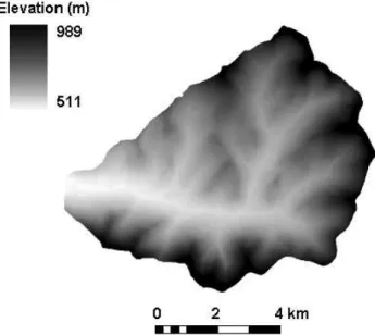
The site for this study was the Town Brook watershed (Fig. 1), in the Catskill Mountain region in New York State. The Town Brook watershed has an area of 37 km2 and an elevation range of 511 to 989 m (Fig. 2). The underlying ge-ology of the watershed was formed during the glacial period, the north facing slopes are generally steep with shallow soils overlaying a dense glacial till and fractured bedrock covered mostly in deciduous and coniferous forests. The south facing slopes are gentler with deeper soils particularly in the lower slope regions and are covered by shrubs, pastures, alfalfa, and corn grown in rotation.
2.2 Satellite images
A time sequence of multi-spectral Landsat 7 ETM+ images was used to identify spatial/temporal changes in the vege-tative cover of Town Brook. The Landsat 7 ETM+ creates
Fig. 2. Digital elevation model of the Town Brook watershed.
images with 30 m×30 m pixel size. The satellite orbital pro-file operates on a 16-day cycle, with each image covering a swath 183 km wide. The spectral range of Band 4 is 780– 900 nm, and is primarily used to estimate biomass, although it can also discriminate water bodies, and soil moisture from vegetation. Band 5 has a spectral range of 1550–1750 nm, and is particularly responsive variations in biomass and mois-ture. Seven cloud-free images were obtained on the follow-ing dates: 27 January 2000, 5 April 2001, 7 May 2001, 8 June 2001, 10 July 2001, 12 September 2001, and 30 Octo-ber 2001. The vegetation and water indices calculated from these images are dependent on precipitation and snow cover on the ground. When the January 2000 image was taken there was snow on the ground. During the rest of the acquisition period in 2001 there was 85 cm of precipitation, which is be-low the thirty year average of 102 cm measured at Delhi, NY, located 20 km west of Town Brook watershed. Only March 2001 and October 2001 had precipitation in excess of the 30 year average. The snow that fell in March 2001 had almost melted by 5 April 2001 when the satellite image was taken, and the May image was taken after a two-week period with-out precipitation. The seven images were used to create the NDWI for the analysis.
2.3 Calculation of NDWI and NDVI
In analogy to the procedure proposed for the MODIS system by Fensholt (2004), the NDWI based on Landsat 7 ETM+ Bands 4 and 5 is defined as follows for each of the seven images:
NDWI = ρ(780−900 nm)−ρ(1550−1750 nm)
ρ(780−900nm)+ρ(1550−1750 nm)
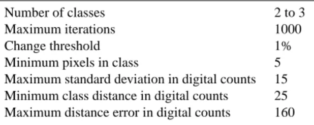
Table 1. Parameter set used in the ISODATA analysis.
Number of classes 2 to 3 Maximum iterations 1000 Change threshold 1% Minimum pixels in class 5 Maximum standard deviation in digital counts 15 Minimum class distance in digital counts 25 Maximum distance error in digital counts 160
where ρ(780−900 nm)is the reflectance in Band 4 of Landsat 7
ETM+, the near infrared band and ρ(1550−1750 nm) is the
re-flectance in Band 5 of Landsat 7 ETM+, the middle infrared band.
Similarly the normalized difference vegetation index (NDVI) that employs the reflectance in Band 4, is defined for the seven images as (Richardson et al., 1992):
NDVI =ρ(780−900 nm)−ρ(630−690 nm)
ρ(780−900 nm)+ρ(630−690 nm)
(2)
where ρ(630−690 nm) is the reflectance in Band 3 of Landsat
7 ETM+, the red band and ρ(780−900 nm)is the reflectance in
Band 4 of Landsat 7 ETM+, the near infrared band.
The NDWI and NDVI are defined in terms of reflectance at the surface while Landsat 7 ETM+ measurements are in terms of radiance measured at the satellite, a value that includes the radiance from the atmosphere including light reaching the sensor, scattering and absorption by gasses, wa-ter vapor, and aerosols (Song et al., 2001). Because of the difficulty of performing an atmospheric correction, it is com-mon practice to use radiance at the detector (after correction for path radiance) instead of reflectance of the target at the surface (Lu et al., 2002; Song et al., 2001). We corrected for path radiance using a dark object subtraction (DOS) cor-rection by calculating the average signal over water bodies for the red and infrared bands and subtracting it from the re-spective red and infrared bands of the entire scene in order to adjust for the atmospheric path radiance. The DOS is the single most important adjustment needed to make the NDWI and NDVI usable when comparing a time sequence of im-ages.
2.4 Unsupervised clustering of NDWI
The three main unsupervised clustering algorithms are K means, Iterative Self Organized Data Analysis Technique A (ISODATA) and the Automatic Classification of Time Series (ACTS) (Tou and Gonzalez, 1972; Viovy, 2000; de Alwis, 2007). In an unsupervised classification, statistical cluster-ing algorithms are used to analyze the digital values in a stack of imagery to determine the number of statistically dis-tinct features (clusters) in the imagery. In this study, an un-supervised ISODATA (ENVI, Research Systems Inc. 2002)
clustering algorithm was used. The ISODATA algorithm is a widely used clustering algorithm that makes a large num-ber of passes through an image using a minimum spectral distance formula to form clusters. It begins with arbitrary cluster means and each time the clustering repeats the means of these clusters are shifted. The new cluster means are used for the next iteration. This iterative process continues until statistically distinct features emerge. The ISODATA tech-nique allows the user to specify the number of classes the data is separated into for clustering within each land cover. The statistical thresholds used to separate the classes in the ISODATA analysis are shown in Table 1.
The land cover map used for this study was obtained by an-alyzing the temporal behavior of vegetation greenness from vegetation indices (NDVI) derived from the same seven im-ages to segregate and identify vegetation with no prior in-formation about the area (de Alwis, 2007). The images were used to identify spatial differences and temporal changes that occurred due to the phenological cycle of vegetative cover over the study site. By analyzing the variations in the NDVI of clusters of pixels over time phenological patterns were ob-tained and distinctive land cover types were identified ac-cordingly. The obtained land cover map was validated us-ing ground truth and air borne imagery. The land cover map based on the phenological variations proved to be better than the available land cover map derived based on spectral clas-sification (de Alwis, 2007). The land cover map based on phenology was able to distinguish the shadowed areas that are often misclassified as evergreen in spectral classification. This was a major advantage of using a classification based on phenology rather than a spectral based classification. Land cover types determined using phenology were arable land, grass/pasture, shrub, deciduous forest, coniferous forest, and mixed forest (Fig. 1). Using masks of each of the land cover types, an image cube or stack was then created for the seven DOS corrected NDWI images. The initial NDWI values that varied from −1 to +1 were linearly stretched between zero and 255 by assigning the least NDWI value in each image cube a value of zero and the maximum NDWI a value of 255. The stretch was necessary because the ISODATA clustering algorithm operates only on integer values. The ISODATA technique divided the NDWI values of the image cubes for each land cover type into two or three NDWI regions with significantly different temporal patterns based on the param-eter thresholds for clustering shown in Table 1. The pattern in NDWI values for the regions represents the temporal vari-ation of surface soil moisture (before leaf on) and leaf water content during the growing season.
2.5 Identification of hydrologically active areas (HAA)
Next we related the NDWI patterns within each land cover to the HAAs in the Town Brook watershed. Town Brook has shallow, highly conductive soils with depths of 30 to 140 cm over a restrictive hardpan. Lateral flow in the shallow surface
Fig. 3. Variation of the Normalized Difference in Water Index
(NDWI) of the two to three homogeneous regions in each of the land cover types (as defined by ISODATA analysis for (a) Arable land,
(b) Deciduous Forests (c) Coniferous Forests (d) Grass/Pasture, (e)
Mixed Forests, (f) Shrub. Blue lines in all figures show the NDWI for predicted saturated zones, red lines show the NDWI for pre-dicted unsaturated zones, in grass/pasture and deciduous forest the light blue and green lines show the NDWI for zones of intermediate saturation. Shown for comparative purposes is the Normalized Dif-ference in Vegetation Index (NDVI) corresponding to each NDWI series.
soil occurs during periods when the precipitation exceeds the potential evaporation and tends to form a saturated area at the bottom of slopes or areas with shallow soils where the stor-age is exceeded. These HAAs saturate during rainfall events and produce runoff. During the period when potential evap-otranspiration exceeds rainfall, the soils dry; interflow drains the water from the soil profile and most of the HAAs dry up and can, in fact, dry out more than other soils in the wa-tershed that are deeper and have a greater storage capacity. During the period when precipitation exceeds evapotranspi-ration we hypothesize that HAA will be detectable on these low storage, shallow soils underlain by a restricting layer. Intuitively, these same areas that saturate during the period when precipitation is greater than evapotranspiration (due to interflow from upslope areas) will be drier during the period where evapotranspiration exceeds precipitation when inter-flow stops (and have lower NDWI values) (Fig. 3). Similarly, regions that had low NDWI during early growing season and high NDWI due to high leaf water content during the growing season are regions with a low propensity to saturate for pro-longed periods as indicated by the better vegetative growth conditions (Fig. 3). The NDWI predicted saturated areas are shown in Fig. 4.
Fig. 4. Normalized Difference in Water Index (NDWI) predicted
saturated (wet) areas for each of the land cover types (Arable land, Mixed Forests, Shrub, Grass/Pasture, Deciduous Forests, and Coniferous Forest).
2.6 Accuracy assessment
Little spatially distributed data on the soil moisture content is readily available; therefore, we propose several ways of test-ing the results: corroboration with existtest-ing hydrologic mod-els and a field survey of saturated areas in the watershed. The remotely sensed HAAs were compared with the distributed output of two simulation models developed for watersheds such as Town Brook, specifically, the Soil Moisture Distri-bution and Routing (SMDR) model (Frankenberger et al., 1999) and Variable Source Loading Function (VSLF) model (Schneiderman et al., 2007). We also used a field survey in the upper reaches of the watershed conducted in 2006 to identify frequently saturated areas. While the simulation models results by no means represent the absolute ground truth we have selected two models that have been shown to capture the evolution of HAAs in the landscape, and should provide an adequate representation of saturated areas. Mod-els based on topographic indices, such as VSLF, or more mechanistic models such as the Soil Moisture Distribution and Routing model (SMDR) (Zollweg et al., 1996; Franken-berger et al., 1999) are two modeling concepts with modest input requirements capable of capturing the spatial distribu-tion of soil moisture levels at the watershed scale. Both mod-els have been shown to identify saturated areas, albeit for different types of systems. Topographic index based mod-els generally assume that a watershed wide water table in-tersects the landscape to produce saturated runoff generating areas and SMDR assumes that these areas are controlled by transient interflow perched on a shallow restricting layer.
The Soil Moisture Distribution and Routing (SMDR) model is a physically-based, fully-distributed model that sim-ulates the hydrology for watersheds with shallow sloping
soils. The model was developed specifically for regions such as Town Brook (Frankenberger et al., 1999). The model com-bines elevation, soil, and land use data, to predict the spatial distribution of soil moisture, evapotranspiration, saturation-excess overland flow (i.e., surface runoff), and interflow throughout a watershed on a daily time step. Soil mois-ture content is predicted for each cell, typically of dimen-sion 10 m. SMDR has been extensively validated in Town Brook (Mehta et al., 2004), and other basins in the region (e.g. Frankenberger et al., 1999; Hively et al., 2005; Eas-ton et al., 2007: more information at http://soilandwater.bee. cornell.edu/).
The Variable Source Loading Function (VSLF) model (Schneiderman et al., 2007), a derivative of the General-ized Watershed Loading Function (GWLF) model (Haith and Shoemaker, 1987), uses the Soil Conservation Curve Number (SCS-CN) (USDA-SCS, 1972) method to predict runoff. The main difference between the VSLF and GWLF approaches to using the SCS runoff equation is that runoff is explicitly attributable to source areas according to a soil to-pographic index distribution rather than by land use and soil type as in original GWLF. Runoff and soil moisture are then distributed throughout the watershed according to a spatially weighted soil topographic index (Lyon et al., 2004) VSLF has been used in the Catskill Mountains to predict hydrology and water quality, and has been validated spatially to predict saturated areas (Schneiderman et al., 2007).
The remotely sensed saturated areas were also compared with a field survey of saturated areas. The field survey was conducted in spring 2006 during the period when HAAs would be most saturated, and should compare reasonably well with HAAs derived by the NDWI. In order to validate the remotely sensed saturated areas the producer’s and user’s accuracies were calculated for comparisons with simulated data and field surveys. The producer’s accuracy for a satu-rated area within a land cover type is defined as the proba-bility within a land cover type that a pixel truly belonging to a saturated area within a land cover type is also mapped as a saturated area within the land cover type, while the user’s accuracy for a saturated area within a land cover type is the probability that a pixel mapped as a saturated area is truly of a saturated area.
3 Results
An average value of NDWI for each of the seven Landsat 7 ETM+ images for the different months was obtained for each of the temporally homogeneous NDWI regions that were identified by the ISODATA clustering method within each of the six land cover types (Table 1). These average NDWI values for the wetness classes are depicted in Fig. 3.
The NDWI time series plots (Fig. 3) show the seasonal dy-namics within and between land cover types. The NDWI for all land covers is elevated in January and April when the soil
is wet. The lowest NDWI occurred in May after a 15 day dry period reduced the moisture content of the soil surface. The NDWI values increase subsequently for June and July due to the increase in leaf water content. The NDWI values for the deciduous and mixed forest decrease at the end in October (due to leaf senescence). The NDWI for the shrub, conif-erous forest, and arable land covers remain stable through the fall, while grass/pasture increase marginally. The slight increase in the NDWI for the grass/pasture is likely due to continued biomass accumulation into the fall, presumably in-creasing the leaf water content.
Comparing the NDWI curves of deciduous forests, grass, shrub, mixed forests, arable land and coniferous forests land cover types in Fig. 3 it is evident that there is a region among all land cover types that is more wet (high NDWI) in the spring than the other homogeneous regions and drier (low NDWI) late in the growing season. This characteristic is con-sistent among all the land cover types. This region is shown in blue in Fig. 3 and, according to our hypothesis, is identi-fied as the wet region in the land cover type. Regions within a land cover type having low surface water content during the early growing season and more leaf water content during the late growing season were identified as dry areas that were favorable for plant growth (due to high leaf water content during the late growing season).
Figure 3 shows the greatest variation in NDWI values be-tween March and April 2001, where snow cover went from 20 cm in March to essentially zero in April. The NDWI is high due to the snow cover and the increase in surface soil moisture from snowmelt. At the same time the evapotranspi-ration loss was small and we expected that the HAAs were fully saturated. The result is that during the early growing season the areas with shallow soil, a high water table, or a large contributing area tended to saturate and were captured in the NDWI images. During the summer when evapotran-spiration exceeds rainfall and interflow supplying water from upslope to the HAAs ceases the differences in NDWI val-ues decreases substantially (Fig. 3). During May and June it is reasonable to assume that the increase in the NDWI in most land covers is due to the increase in biomass, and sub-sequent leaf water content from maturing vegetation. Dur-ing the summer, it is of interest to note that the moisture content in the HAAs that were saturated during the spring snowmelt decreases below that of the remaining land cover types (Fig. 3) because the HAA soils are shallower and have less storage.
As a matter of interest, the NDVI values are also calcu-lated for the NDWI wetness classes and show the opposite behavior from that of the NDWI. The NDVI values are low in January and March when there is little biomass and then increase during the rest of the year when plant growth re-sumes. Detailed information on the differences in NDVI values between land cover types can be found in de Alwis (2007). What is important here is that the different wet-ness index classes showed few differences in NDVI values.
Overall accuracy 0.78 VSLF wet NDWI wet Overlap PA UA Deciduous forest 1723 3783 1522 0.88 0.40 Grass 3889 4170 2632 0.68 0.63 Shrub 7320 6139 5883 0.80 0.96 Mixed forest 2776 2378 2337 0.84 0.98 Arable land 1365 1255 1244 0.91 0.99 Coniferous forest 1041 721 703 0.68 0.98 Total 18 114 18 446 14 321 Overall accuracy 0.79 VSLF wet SMDR wet Overlap PA UA Deciduous forest 1723 1111 1063 0.62 0.96 Grass 3889 5150 3087 0.79 0.60 Shrub 7320 7196 6865 0.94 0.95 Mixed forest 2776 2796 2744 0.99 0.98 Arable land 1365 1378 1363 1.00 0.99 Coniferous forest 1041 341 141 0.14 0.41 Total 18 114 17 972 15 263
During January and April when there is little biomass (except for coniferous forest), the NDVI values should be the same. During the summer the leaf area index for all land covers is greater than three and it is difficult to discriminate among differences in the NDVI signal. The insensitivity to moisture content makes the NDVI signal a good proxy to distinguish land cover types but a poor predictor of moisture status.
3.1 Validation
The main difficulty in comparing the NDWI predicted HAAs is that the remotely sensed saturated areas are static in time and represent an average saturation risk for the year of ob-servation while the saturated areas predicted by SMDR and VSLF are continuous, and dynamic in time. That being said, the NDWI saturated areas should represent areas of the land-scape most prone to frequent saturation. To compare the temporally dynamic prediction made by SMDR and VSLF we aggregated predictions during the spring for SMDR and VSLF (March–June 2001), which represents the most
prob-able saturated period in this region. The simulated satura-tion degree maps for SMDR and VSLF were stacked and an average saturation degree was calculated for each of the 10 m×10 m pixels. We resampled the 30 m×30 m NDWI pixels to 10 m×10 m pixel size to compare among models. The area of each specific land cover in Town Brook was cal-culated and a ratio of total land cover to NDWI saturated area was derived. For example, deciduous forest covers 21 677 pixels of Town Brook, of which 3183 are predicted as sat-urated by the NDWI, that is, 17.5% of the deciduous forest in Town Brook is predicted as an HAA. Then these areas were extracted independently for each land cover from the SMDR or VSLF saturation degree maps. We assume that the pixels from the SMDR and VSLF maps with the high-est saturation degree, corresponding to the fraction of the re-motely sensed land cover that was saturated, should theoret-ically correspond with the remotely sensed data (the 17.5% of cells with the highest saturation degree for deciduous for-est from SMDR and VSLF). This allowed comparison of the potentially saturated areas on an areal basis.
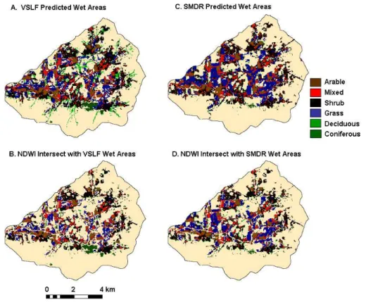
Fig. 5. (a) Saturated areas by land cover predicted by the Variable Source Loading Function (VSLF) model: (b) Intersection of saturated
areas predicted by the NDWI and those predicted by VSLF: (c) saturated areas by land cover predicted by the Soil Moisture Distribution and Routing (SMDR) model: (d) Intersection of saturated areas predicted by the NDWI and those predicted by SMDR.
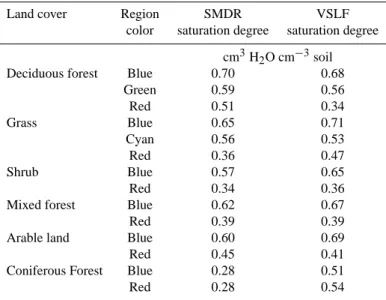
The region maps representing the temporally homoge-neous NDWI regions for each land cover type were overlaid on the saturation degree map and the mean saturation de-gree value within each of the regions was calculated. Results of this comparison are shown in Table 2. In all of the land cover types (except coniferous forests) it seems that the com-mon characteristic of the homogeneous regions that are wet (represented by the blue curves in Fig. 3) in the early grow-ing season and dry in the late growgrow-ing season have higher saturation degrees than those areas predicted as dry. The remotely sensed saturated areas are shown in Fig. 4. The intersection of the NDWI saturated areas and the SMDR and VSLF saturated areas are shown in Fig. 5. The extent of the remotely sensed NDWI based saturated area predic-tions for the arable land, deciduous forest, mixed forest, and shrub were extracted from the GIS and the producer (er-ror of omission) and users (er(er-ror of commission) accuracy were tabulated. Thus, we have a measure of where the re-motely sensed NDWI saturated areas agree with the SMDR or VSLF saturated areas (producers’ accuracy Table 2). The remotely sensed saturated areas generally agree well with the model predictions with overall accuracies of 0.78 and 0.79 for SMDR and VSLF, respectively. However, saturated areas in the deciduous forest land cover predicted by the remote sensing method do not agree as well with SMDR and VSLF
(Fig. 5, Table 2). The positions of the NDWI saturated ar-eas within the deciduous forests were accurately predicted (producer’s accuracy, Table 2) but their extent was over pre-dicted compared to the modeled saturated areas (user’s ac-curacy, Table 2). The main discrepancy between the NDWI saturated areas and the modeled saturated areas is likely that the LAI is greater than six in the forest and the NDWI be-comes saturated and unable to discriminate saturated areas. Additionally, the moisture status of the soil surface likely has limited influence on the water content of the deciduous trees, as they can derive water from deeper in the soil, and the leaf water status may be more affected by regional groundwater dynamics then surface phenomena.
To test the above hypothesis further the SMDR and VSLF predicted saturation degree were compared to the remotely sensed homogeneous regions (Table 3). According to the hypothesis within a land cover type a higher surface water content during the early growing season and lower leaf wa-ter content during the late growing season indicates a hydro-logically sensitive (saturated) area, that are not favorable for plant growth (represented by the blue curve in Fig. 3). In-deed, NDWI predicted saturated areas had a higher soil mois-ture level as predicted by SMDR and VSLF (Table 3).
Due to the uncertainty inherent in the spatial predictions of any model we conducted a field survey of saturated areas in
Red 0.36 0.47 Shrub Blue 0.57 0.65 Red 0.34 0.36 Mixed forest Blue 0.62 0.67 Red 0.39 0.39 Arable land Blue 0.60 0.69 Red 0.45 0.41 Coniferous Forest Blue 0.28 0.51 Red 0.28 0.54
Table 4. Producers (PA) and Users Accuracy (UA) assessment of remotely sensed saturated areas compared to the equivalent areal extent by
land cover of saturated areas mapped using a Garmin GPS (GPSmap 60C). The mapped saturation areas are considered ground truth for the classification comparison.
Land cover Mapping wet NDWI wet Overlap PA UA Deciduous forest 242 214 103 0.43 0.48 Grass 67 195 48 0.72 0.25 Shrub 266 185 132 0.5 0.71 Mixed forest 13 39 11 0.85 0.28 Arable land 0 2 0 0 0 Coniferous forest 61 111 21 0.34 0.19 Total 649 746 315 Overall accuracy 0.49
the south eastern portion of Town Brook on 28–30 April 2006 using a Garmin GPS (GPSmap 60C, Garmin Inc.) with 2 m horizontal accuracy. Areas were deemed saturated if there were signs of surface saturation or water tables close to the ground surface (e.g. bootprints would fill with water). Man-ual delineations of HAAs from the field mapping survey of the Town Brook watershed are shown in Fig. 6. The pro-duced map of saturated areas was converted into a raster file with 30 m×30 m resolution and classified according to the land cover types derived from the remote sensing data (de Alwis, 2007). This map was compared with the 7 May 2001 NDWI derived image. The area of each specific land cover from the May NDWI image within the survey area was cal-culated and a ratio of total mapped saturation area to NDWI saturated area was derived, with the corresponding errors of
omission and commission calculated (Table 4). Since satu-rated areas generally occur in the same location from year to year, we expected a general agreement on the location of these saturated areas but not necessarily on the extent of the saturated areas, since measurements taken in 2006, were made under relatively wet conditions and the NDWI values, were taken on 7 May 2001, following two weeks of dry con-ditions.
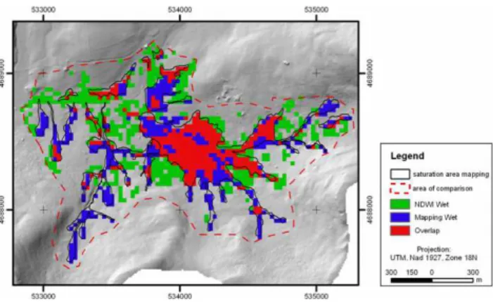
Indeed, we found that the general location of the saturated areas were predicted well but the mapped extent agreed less well with an overall accuracy of 49% (Fig. 6, Table 4). As Table 4 shows, the NDWI predicted a generally larger ex-tent of saturated areas compared to the field survey. Similar to the comparison with the simulation model, the conifer-ous forest was predicted poorly with low user’s accuracies
Fig. 6. Field survey delineated saturated areas in a portion of the
Town Brook watershed compared to the NDWI predicted saturated area of the 7 May 2001 image.
(Table 4). The correspondence between field observation and NDWI based predictions for land cover classes of decidu-ous forest and shrub show good agreements with accuracies of 48% and 71% respectively. As Fig. 6 illustrates, most of the spatial disagreement between NDWI derived and mapped saturated areas results from an over-prediction of saturation areas in the grass land cover classes and an under-prediction in the deciduous forest and shrub land cover classes. The main discrepancy between the NDWI saturated areas and the mapped saturated area extents occurs in the coniferous for-est land cover class, where the NDWI reached the highfor-est (positive) value because of the high LAI. Similar to decid-uous forest during the growing season, the leaf water status of the coniferous forest is most likely less affected by short term changes in soil saturation as in other vegetation classes (grass/pasture, shrub, deciduous forest).
4 Discussion
In theory, areas within a land cover type situated on a steep slope, deep soils, a high permeability, and a low contribut-ing area should remain drier than those areas with shallow slopes and soils, low permeability, and a large contributing area. In such steep-sloped areas within each landcover type the NDWI is lower during the early spring. The depth of the soil, a proxy for soil storage capacity, directly influences the leaf water content in late summer and during dry peri-ods, while the depth of the soil is inversely proportional to the wetness of the soil in early spring.
Analysis of the NDWI data during a complete phenologi-cal cycle within a land cover type highlights significant hy-drological characteristics within the land cover. While the NDWI varies proportionally with the surface water content before leaf on (early spring) and leaf water content during leaf on (summer), the largest differences were consistently detected during the spring (Fig. 3), consistent with the other measurements and model analysis from the region. There
were few differences detected during the summer and early fall periods, as watersheds in this region tend to dry out dur-ing the period from June to October when evapotranspiration is greater than precipitation. However, there were differences in the NDWI for the arable and pasture land covers during the summer. Specifically, the areas with a higher NDWI in the spring had considerably lower values than other areas in the summer (Fig. 3). There are likely numerous explana-tions for this observation, but several appear more probable. First in these HAAs, the shallow, low storage soils are prone to drying out, providing inadequate plant available water to produce similar biomass as the non-saturation prone areas. Second, and related to the first, the arable and pasture land covers typically have less developed root systems and probe the soil less aggressively for moisture than the forest or shrub type land covers, making them more susceptible to moisture stress. In order to capture HAAs using a NDWI a compar-ison of images acquired during wet and dry periods during leaf on season (summer) best support the differentiation of soil moisture and leaf water differences among all land cover classes.
The time series of the NDWI images exhibit characteris-tics consistent with the hydrologic setting of the land covers considered. Interestingly coniferous forest behaved differ-ently than the other land cover types. The region that had high NDWI during the early growing season and low NDWI during the late growing season that was hypothesized as the wet area (HAA) was predicted as dry according to the hydro-logical models. The high NDWI measured during the spring was clearly not due to the soil surface water content as the satellite would not sense the soil surface as the LAI would be well above six. Another reason could be due to the fact that NDWI responds differently to evergreen needles. Fur-ther study needs to be done to explain this atypical behavior among the coniferous forests.
A significant issue in using this approach is the availabil-ity of the imagery for a single year. The Landsat 7 ETM+ satellite collects imagery over the study area once every 16 days or about 23 times per year. The maximum amount of data that would be available to create a one-year time series would be 23 images. In practice, getting a sequence of six to eight images that are roughly equally-spaced through the year could be difficult with Landsat 7 ETM+ data. However, the Landsat 7 ETM+ data were selected because its spatial resolution matched the need to identify relatively small re-gions of uniform land cover classes. Where spatial resolution is not so critical, there are satellite-based instruments (e.g. MODIS with 1 km pixels and appropriate spectral bands) that provide coverage every one to two days, and should be capa-ble of providing much more detailed time series. However, the resolution is such that delineating saturated areas can be difficult (only 37 pixels for Town Brook). This invites the question of how many images are actually required and what the critical time periods are. It is clear that the April image was imperative to capture the saturated areas in the watershed
2011. However, several other sensors can provide promis-ing sources of Landsat-like data, includpromis-ing the China/Brazil Earth Resources Satellite (CBERS-2), and the Indian Remote Sensing (IRS-P6) ResourceSat-1 satellite.
This series analysis of remotely sensed spectral data has never been used for the identification of HAAs but holds great potential, particularly at large scale since the deriva-tion is independent of field measurements and hydrological parameters. However since this study was conducted in a temperate humid region of the country this method is based specifically on vegetation and likely cannot be used to predict saturated areas in semi arid and arid areas, or areas where runoff is generated by infiltration excess processes and not from saturated areas of the landscape. The method might successfully be applied to determine relative differences in moisture contents in many areas, VSA or otherwise. Further work is necessary to investigate application of this method to other regions.
5 Conclusions
Based on the temporal pattern of a wetness index derived from remotely sensed satellite imagery we were able to iden-tify HAAs using an unsupervised classification technique. This method is advantageous because it allows identification of HAAs independent of field measurements at a high spa-tial resolution. The two images in the early and late growing season contributed substantially to the accuracy of the results and were critical in the sequence, since during these periods plant growth is rapid and reflective of the stresses to which they are subjugated. The April image collected when there was four cm of snow on the ground, and the May image that was taken after 15 days of drought contributed substantially to the analysis. The largest variation among each homoge-neous land cover type was seen on the April image with snow cover. The May image showed the NDWI to decrease due to the 15 precipitation free days prior to the image; the increase in NDWI thereafter was due to increases in the leaf water content, particularly for the arable land and pasture land cov-ers.
Beven, K. J.: Rainfall-runoff modeling: the primer, John Wiley & Sons, LTD, Chichester, England, 360 pp, 2001.
Bindlish, R., Jackson, T. J., Wood, E., Huilin, G., Starks, P., Bosch, D., and Lakshmi, V.: Soil moisture estimates from TRMM Mi-crowave Imager observations over the Southern United States, Remote Sens. Environ., 85, 507–515, 2003.
Ceccato, P., Flasse, S., Tarantola, S., Jacquemoudy, S., and Gr’egoire, J. M.: Detecting vegetation leaf water content using reflectance in the optical domain, Remote Sens. Environ., 77, 22– 33, 2001.
Chen, J. M. and Cihlar, J.: Retrieving leaf area index of boreal conifer forests using LANDSAT TM images, Remote Sens. En-viron., 55, 153–162, 1996.
Cohen, W. B., Maiersperger, T. K., Gower, S. T., and Turner, D. P.: An improved strategy for regression of biophysical variables and LANDSAT ETM+ data, Remote Sens. Environ., 84, 561–571, 2003.
de Alwis, D. A.: Identification of hydrologically active areas in the landscape using satellite imagery, PhD Dissertation, Cornell Uni-versity, Ithaca, NY, 2007.
De Jong, R., Shields, J. A., and Sly, W. K.: Estimated soil water reserves applicable to a wheat-fallow rotation for generalized soil areas mapped in southern Saskatchewan, Canadian J. Soil Sci., 64(3), 667–680, 1984.
Dunne, T. and Black, R. D.: Partial area contributions to storm runoff in a small New England watershed, Water Resour. Res., 6, 1296–1311, 1970.
Dunne, T. and Leopold, L: Water in Environmental Planning, W. H. Freeman & Co., New York. 818 pp, 1978.
Easton, Z. M., G´erard-Marchant, P., Walter, M. T., Petrovic, A. M., and Steenhuis, T. S.: Hydrologic assessment of an urban variable source watershed in the northeast United States, Water Resour. Res., 43, W03413, doi:10.1029/2006WR005076, 2007. Farrar, T. J., Nicholson, S. E., and Lare, A. R.: The influence of
soil type on the relationships between NDVI, rainfall, and soil moisture in semiarid Botswana, Remote Sens. Environ., 50(2), 121–133, 1994.
Fassnacht, K. S., Gower, S. T., MacKenzie, M. D., Nordheim, E. V., and Lillesand, T. M.: Estimating the leaf area index of north cen-tral Wisconsin forests using the LANDSAT Thematic Mapper, Remote Sens. Environ., 61, 229–245, 1997.
Fensholt, R.: Earth observation of vegetation status in the Sahe-lian and Sudanian West Africa, comparison of Terra MODIS and NOAA AVHRR satellite data, Int. J. Remote Sens., 25(9), 1641– 1659, 2004.
Foody, G. M. and Arora, M. K: Incorporating mixed pixels in the training, allocation and testing stages of supervised classifica-tions, Pattern Recognition Lett., 17, 1389–1398, 1996.
Frankenberger, J. R., Brooks, E. S., Walter, M. T., Walter, M. F., and Steenhuis, T. S.: A GIS based variable source area hydrology model, Hydrol. Processes, 13, 805–822, 1999.
Friedl, M. A., Michaelsen, J., Davis, F. W., Walker, H., and Schimel, D. S.: Estimating grassland biomass and leaf area index using ground and satellite data, Int. J. Remote Sens., 15, 1401–1420, 1994.
Gao, B.: NDWI. A normalized difference water index for remote sensing of vegetation liquid water from space, Remote Sens. En-viron., 58(3), 257–266, 1996.
Gates, D., Keegan, J. J., Schleter, J. C., and Weidner, V. R.: Spectral properties of plants, Appl. Optics, 4, 11–20, 1965.
Guha, A. and Lakshmi, L.: Sensitivity, spatial heterogeneity, and scaling of C-Band microwave brightness temperatures for land hydrology studies, IEEE Trans. Geosci. Remote Sensing, 40(12), 2626–2635, 2002.
Haith, D. A. and Shoemaker, L. L.: Generalized Watershed Loading Functions for stream flow nutrients, Water Resour. Bull., 23(3), 471–478, 1987.
Hively, W. D., Gerard-Marchant, P., and Steenhuis, T. S.: Dis-tributed hydrological modeling of total dissolved phosphorus transport in an agricultural landscape, part II, dissolved phospho-rus transport, Hydrol. Earth Syst. Sci., 10, 263–276, 2006, http://www.hydrol-earth-syst-sci.net/10/263/2006/.
Hunt Jr., E. R., Rock, B. N., and Nobel, P. S.: Measurement of leaf relative water content by infrared reflectance, Remote Sens. Environ., 22, 429–435, 1987.
Karnieli, A., Kaufman, Y., Remer, L., and Wald, A.: AFRI – aerosol free vegetation index, Remote Sens. Environ., 77(1), 10– 21, 2001.
Kerr, Y. H.: Soil moisture from space: Where are we?, Hydrogeol-ogy J., 15, 117–120, 2007.
Killelea, M.: Carbon storage in New York State forestland, Ph.D. Dissertation, Cornell University, Ithaca, NY, USA, 2005. Law, B. E. and Waring, R. H.: Remote sensing of leaf area index
and radiation intercepted by understory vegetation, Ecol. Apps., 4, 272–279, 1994.
Le Hegarat-Mascle, S., Bloch, I., and Vidal-Madjar, D.: Applica-tion of Dempster-Shafer evidence theory to unsupervised clas-sification in multisource remote sensing, IEEE Trans. Remote Sens., 35, 1018–1031, 1997.
Lu, D., Mausel, P., Brondizio, E., and Moran, E.: Assessment of atmospheric correction methods for Landsat TM data applicable to Amazon basin LBA research, Int. J. Remote Sens., 23, 2651– 2671, 2002.
Lyon, S. W., Walter, M. T., Gerard-Marchant, P., and Steenhuis, T. S.: Using a topographic index to distribute variable source area runoff predicted with the SCS curve-number equation, Hydrol. Processes, 18, 2757–2771, 2004.
Mehta, V. K., Walter, M. T., Brooks, E. S., Steenhuis, T. S., Walter, M. F., Johnson, M., Boll, J., and Thongs, D.: Application of SMR to modeling watersheds in the Catskill Mountains, Environ, Model. Assess., 9, 77–89, 2004.
Needelman, B. A., Gburek, W. J., Petersen, G. W., Sharpley, A. N., and Kleinman, P. J. A.: Surface runoff along two agricultural hillslopes with contrasting soils, Soil Sci. Soc. Am. J., 68, 914–
923, 2004.
Nicholson, S. E. and Farrar, T. J.: The influence of soil type on the relationships between NDVI, rainfall, and soil moisture in semiarid Botswana, Remote Sens. Environ., 50, 107–120, 1994. Research Systems, Inc. ENVI Users Manual, What’s new in ENVI
4.0 ENVI Version 4 Edition, Boulder, Colorado, 2002.
Richardson, A. J., Wiegand, C. L., Wanjura, D. F., Dusek, D., and Steiner, J. L.: Multisite analyses of spectral-biophysical data for Sorghum, Remote Sens. Environ., 41(1), 71–82, 1992.
Schmugge, T.: Remote sensing of soil moisture, in: Hydrological Forecasting, edited by: Anderson, M. G. and Burt, T. P., Wiley, New York, 101–124, 1985.
Schneiderman, E. M., Steenhuis, T. S., Thongs, D. J., Easton, Z. M., Zion, M. S., Mendoza, G. F., Walter, M. T., and Neal, A. L.: Incorporating variable source area hydrology into the curve number based Generalized Watershed Loading Function model, Hydrol. Processes, in press, available online at: http://www3. interscience.wiley.com/cgi-bin/jissue/89013836, 2007.
Song, C., Woodcock, C. E., Seto, K. C., Pax-Lenney, M., and Ma-comber, S. A.: Classification and change detection using Landsat TM data: when and how to correct for atmospheric effects, Re-mote Sens. Environ., 75(2), 230–244, 2001.
Timlin, D. J., Pachepsky, Y., Walthall, C. L., and Loechel, S. E.: The use of a water-budget model and yield maps to characterize water availability in a landscape, Soil and Tillage, 58, 219–231, 2001.
Tou, J. T. and Gonzalez, R. C.: Recognition of handwritten charac-ters by topological Feature extraction and multilevel categoriza-tion, IEEE Trans. Computers, 21, 776–787, 1972.
Tucker, C. J.: Remote sensing of leaf water content in the near in-frared, Remote Sens. Environ., 10, 23–32, 1980.
USDA-SCS (Soil Conservation Service): National Engineering Handbook, Part 630 Hydrology, Section 4, Chapter 10, 1972. Viovy, N.: Automatic Classification of Time Series (ACTS): a new
clustering method for remote sensing time series, Int. J. Remote Sens., 21, 1537–1560, 2000.
Wagner, W., Naeimi, V., Scipal, K., de Jeu, R., and Martinez-Fernandez, J.: Soil moisture from operational meteorological satellites, Hydrogeology J., 15, 121–131, 2007.
Wang, J. R. and Schmugge, T. J.: An empirical model for the com-plex dielectric permittivity of soils as a function of water content, IEEE Trans. Geosci. Remote Sens., 18(4), 288–295, 1980. Wang, J., Price, K. P., and Rich, P. M.: Spatial patterns of NDVI
in response to precipitation and temperature in the central Great Plains, International J. Remote Sens., 22(18), 3827–3844, 2001. Whiting, M. L., Lin, L., and Ustin, S. L.: Predicting water content using Gaussian model on soil spectra, Remote Sens. Environ., 89(4), 535–552, 2004.
Xiao, X., Boles, S., Liu, J. Y., Zhuang, D. F., and Liu, M. L.: Char-acterization of forest types in Northeastern China, using multi-temporal SPOT-4 VEGETATION sensor data, Remote Sens. En-viron., 82, 335–348, 2002.
Yang, J. P., Ding, Y. J., and Chen, R. S.: Spatial and temporal of variations of alpine vegetation cover in the source regions of the Yangtze and Yellow Rivers of the Tibetan Plateau from 1982 to 2001, Environ. Geol., 50(3), 313–322, 2006.
Zollweg, J. A., Gburek, W. J., and Steenhuis, T. S.: SMoRModA GIS-integrated rainfall-runoff model applied to a small northeast U.S. watershed, Trans. ASAE, 39, 1299–1307, 1996.