A two-phase model for compaction and damage 1. General Theory

HAL Id: hal-02046735

https://hal.archives-ouvertes.fr/hal-02046735

Submitted on 25 Jan 2021

HAL is a multi-disciplinary open access

archive for the deposit and dissemination of

sci-entific research documents, whether they are

pub-lished or not. The documents may come from

teaching and research institutions in France or

abroad, or from public or private research centers.

L’archive ouverte pluridisciplinaire HAL, est

destinée au dépôt et à la diffusion de documents

scientifiques de niveau recherche, publiés ou non,

émanant des établissements d’enseignement et de

recherche français ou étrangers, des laboratoires

publics ou privés.

A two-phase model for compaction and damage 1.

General Theory

D. Bercovici, Y. Ricard, G. Schubert

To cite this version:

D. Bercovici, Y. Ricard, G. Schubert. A two-phase model for compaction and damage 1. General

Theory. Journal of Geophysical Research : Solid Earth, American Geophysical Union, 2001, 106 (B5),

pp.8887-8906. �10.1029/2000JB900430�. �hal-02046735�

A two-phase model for compaction and damage

1. General Theory

David Bercovici •

Department of Geology and Geophysics, University of Hawai'i at Manoa, Honolulu, Hawaii

Yanick Ricard

Laboratoire de Sciences de la Terre, Ecole Normale Sup6rieure de Lyon, Lyon, France

Gerald Schubert

Department of Earth and Space Sciences, University of California, Los Angeles, California

Abstract. A theoretical model for the dynamics of a simple two-phase mixture is presented. A classical averaging approach combined with symmetry arguments is used to derive the mass, momentum, and energy equations for the mixture. The theory accounts for surficial energy at the interface and employs a nonequilibrium equation to relate the rate of work done by surface tension to the rates of both pressure work and viscous deformational work. The resulting equations provide a basic model for compaction with and without surface tension. Moreover, use of the full nonequilibrium surface energy relation allows for isotropic damage, i.e., creation of surface energy through void generation and growth (e.g., microcracking), and thus a continuum description of weakening and shear localization. Applications to compaction, damage, and shear localization are investigated in two companion papers.

1. Introduction

The dynamics of two-component, or two-phase (and in general multiphase), media is a complex and well-studied

field [see Drew and Passman, 1999] with innumerable natu- ral applications to sediment and soil mechanics [Biot, 1941; Hill et al., 1980; Birchwood and Turcotte, 1994; see Furbish,

1997, and references therein], glaciology [Fowler, 1984], oil recovery and magma dynamics [McKenzie, 1984; Spiegel- man, 1993a, 1993b, 1993c], crystallization in metal alloys [Ganesan and Poirier, 1990], and slurries [Loper, 1992]. Analysis of dilatant plasticity [Mathur et al., 1996], rate- and-state friction models of earthquake dynamics [Segall and Rice, 1995; Sleep, 1995, 1997, 1998], and void-volatile self-lubrication models of the generation of plate tectonics from mantle flow [Bercovici, 1998] also employ the concept of two phases by relating porosity to a weakening effect or a

state variable.

One of the most complex issues in the mechanics of two-

phase media concerns the physics of the interface between

the phases [Groenwald and Bedeaux, 1995; Osmolovski,

1997]. Interface and surface dynamics is also a vital field

1 Now at Department of Geology and Geophysics, Yale University, New

Haven, Connecticut.

Copyright 2001 by the American Geophysical Union.

Paper number 2000JB900430.

0148-0227/01/2000JB 900430509.00

for the study of rock mechanics and material science [Jaeger

and Cook, 1979; Atkinson, 1987; Atkinson and Meredith,

1987]. One of the primary manifestations of an interface is its intrinsic surface energy, partially expressed as sur-

fhce tension. Surface energy and tension are relevant both

for melt dynamics in the process of crystallization [Tiller, 1991a, 1991b; Lasaga, 1998] and percolation under cap- illary forces [Harte et al., 1993; Stevenson, 1986]. It is also generally recognized that the damage of materials in- volves the generation of a surface energy on newly devel- oped cracks and voids [Griffith, 1921; Jaeger and Cook,

1979; Atkinson, 1987; Atkinson and Meredith, 1987].

The effects of surface tension have been considered for

two-phase systems [Drew, 1971; Drew and Segel, 1971;

Stevenson, 1986; Ni and Beckermatt, 1991; Straub, 1994; Groenwald and Bedeaux, 1995; Osmolovski, 1997], although,

to our knowledge, they have not been self-consistently incor- porated in a closed, fully three-dimensional, two-phase con- tinuum theory. In this paper we derive the simplest possible general equations for a two-phase medium, accounting for the possibility of surface free energy existing on the inter-

face between the two media. Although this surface energy

is often considered to be in static equilibrium with the net work done by the pressure fields of the two phases [e.g., Ni and Beckerman, 1991], we propose a more general relation in which surface energy is generated through nonequilibrium energy sources such as deformational work. Thus the theory provides a simple model not only of compaction with and

without surface tension but also of the creation of surface

8888 BERCOVICI ET AL.: TWO-PHASE COMPACTION AND DAMAGE, 1, THEORY

energy through deformation, and hence microcracking and damage. However, the theory is based on viscous fluid me-

chanics, and thus it is most applicable to viscous and/or long- timescale mantle-lithosphere processes, such as magma dy-

namics and plate boundary formation through ductile local-

ization mechanisms.

Although some of the equations derived in this model dif-

fer little from those derived previously [Drew, 1971; Drew

and Segel, 1971; Loper and Roberts, 1978; Hills et al., 1983, 1992; McKenzie, 1984; Fowler, 1984, 1990a, 1990b; Richter and McKenzie, 1984; Ribe, 1985, 1987; Bennon and Incr- opera, 1987; Scott, 1988; Scott and Stevenson, 1989; Gane- san and Poirier, 1990; Poirier et al., 1991; Loper, 1992; Tur- cotte and Phipps Morgan, 1992; Spiegelman 1993a, 1993b, 1993c; Gidaspow, 1994; Schmeling, 2000; see Drew and

Passman, 1999], others are signficantly different or are en- tirely new. Thus it is necessary that the formalism for arriv-

ing at the theory be established; admittedly, this formalism is

not in itself new, so its presentation will be as brief as possi- ble. In the following subsections we will derive conservation

laws, which, in two-phase theory, involve a particular aver- aging scheme [Drew, 1971;Drew and Segel, 1971; Ganesan and Poirier, 1990; Ni and Beckerman, 1991 ]. Although the averaging method has been discussed elsewhere, we will re-

quire it to carry out some of the derivation; thus we describe

it by example, i.e., through consideration of the mixture's

properties and the conservation of mass law.

To keep our theory as simple as possible, we make the

following assumptions:

1. Both media have constant densities and are thus incom-

pressible.

2. Both media behave as highly viscous fluids (such that inertia and acceleration are neglected, i.e., forces are always in balance), and their individual viscosities are constant.

3. The two-phase mixture remains isotropic, i.e., on av- erage (see below for how the average is defined), pores and

grains are not collectively elongated in a preferred direction. (Some discussion of anisotropy, however, is included in this development.)

Nevertheless, the two-phase mixture will have noncon- stant effective density and viscosity. Other simplifying as-

sumptions will be stated as necessary.

stant. The two phases have true (or microscopic) velocities,

•ri and

•rm within

their

respective

volumes,

and

similarly

for

pressures and stresses. However, in a two-phase or mixture theory, we cannot know the location of every parcel of fluid or matrix; thus we must average all quantities over some vol- ume; the size of this volume determines the validity of the continuum limit for two-phase theory. This limit is analo- gous to that for single-phase continuum theory in which the volume over which properties are averaged must be large enough to contain sufficient numbers of molecules but must also be small enough to distinguish gradients in properties.

In two-phase theory the volume must be large enough to con-

tain sufficient numbers of pores or grains but small enough to resolve gradients. As pore and grain sizes can become macroscopic, the volume size is potentially very constrained,

and thus it is much easier to violate the two-phase contin-

uum limit [Bear, 1988; Furbish, 1997; Drew and Passman,

1999].

Once the two materials, the matrix and fluid, are com-

bined, the mixture has additional properties prescribed by a distribution function which locates pores of fluid or grains

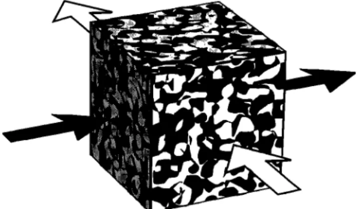
of matrix (Figure 1 ); we define this distribution function 0

which is 1 inside the fluid pores and 0 in the matrix [Drew, 1971; Drew and Segel, 1971; Fowler, 1984; Ganesan and Poirier, 1990; Ni and Beckerman, 1991]. The function 0 is used to average properties over fluid or matrix volumes. In particular, porosity, i.e., the volume fraction of fluid (assum- ing the matrix is saturated), is an average quantity defined

as

1 • OdV,

(1)

where 8V is the total volume of an element of mixture. The

masses of fluid and matrix in the volume 8V are thus the

integrals of py and pm over the fluid and matrix volumes,

respectively

2. Mixture Properties

2.1. Phase Properties and Averaging

We define the two phases as fluid and matrix to be consis- tent with much of the classic literature on this topic. How- ever, we derive all equations to maintain their symmetry; that is, until we make a symmetry-breaking assumption about an extreme difference between the fluid phase and matrix phase, they are strictly speaking both incompressible, cons- tant-viscosity fluids, and thus how we label them should be irrelevant. Therefore an interchange of labels must result in the same equations. We will refer to this symmetry as "ma-

terial invariance."

We define the fluid and matrix phases to have densities

t9f and Pm and viscosities •f and •m, all of which are con-

Figure 1. Schematic of a control volume t$V with a mixture

of fluid (white) and matrix (black). Shading also represents

the distribution function 0 which is 1 in the fluid and 0 in

the matrix. The curve which marks the boundary between

black and white as viewed in the figure is the intersection of the interface between the phases and the surface of the con- trol volume, as denoted by Ci in (25). Arrows illustrate the flux of fluid and matrix mass, momentum or energy through

exposures of fluid and matrix at the surface of the control

Mf-f6vPfOdV,

Mm-f6

V

which,

because

the densities

are constant,

are simply

Mf =

ckpf6V and Mm = (1 - c))pm6V. The fluid velocity aver- aged over the fluid volume is vf, defined such that

1 es

øat5

Ovs

- 3-ff v

where vf is often referred to as the interstitial velocity, while

½vf is the Darcy velocity. The matrix velocity v• is simi-

larly defined such that

1 f• %•(1-O)dV.

U

(4)

Since the two media are assumed incompressible, their true

velocities

•'• and •'• are solenoidal

(V ß •'• = V. •'• =

0); however, the averaged velocities v f and v• are not solenoidal since they have been averaged over pore or grain

volumes that are variable in space and time.

2.2.1. Constant C•o. The constant ao is an important property throughout the development and application of this

model; it has units of m -i and is inversely related to charac-

teristic pore and grain size. Although we cannot offer an

exact demonstration of this relation, it can be understood by a very simple conceptual example [after Spry, 1983). We consider a volume where the pores and grains are the same shape and size for all porosities and these grains and pores fit together exactly; for simplicity, we choose a cubi-

cal volume with sides L and cubical pores and grains of side

d < < L. The total number of pores and grains together is

Ntot = (L/d) a, and if we have

N pores,

then

the porosity

is ½ = N/Ntot. For a small number of pores (N << Ntot)

the net interfacial surface area is Ai = N6d 2, while for a large number of pores (or small number of grains) where

N -+ Ntot we have

Ai = (Ntot- N)6d 2 (for example,

with

Ntot - I pores, there is just one cubic grain of side d). Thus a symmetric formula that gives both limits for Ai would

be Ai = [N(Ntot- N)/Ntot]6d

2, or since

N = Ntot0,

Ai = NtotO(1

- O)6d

2. The interface

area

per volume

is

2.2. Interfacial Area Density

An additional property of the mixture concerns the fabric of the mixture which is specified by the location and orien- tation of the interface between the two phases. The interface location and orientation are given by V0, which is in essence a Dirac 6 function, centered on the interface, times the unit normal to the interface (in fact, pointing from the matrix to the fluid, in the direction of increasing 0). Thus the net in- terface area within a volume 6V is simply

IVOIdV. (5)

However, in a mixture formalism we cannot know the loca- tion and orientation of the interface between fluid and ma-

trix, and thus we must define an averaged property. In this

paper we assume isotropy of the interface (i.e., on average, it has no preferred direction) and that in the control vol-

ume 6V, there is an average interfacial area per unit volume, a - 6Ai/6V [see also Ni and Beckerman, 1991). Since the system is isotropic, we assume that this single quantity

is sufficient to characterize the density of the interface. The

area density a is necesarily a function of porosity since it must vanish when the medium becomes a single-phase sys-

tem, i.e., when ½ - 0 or 1. As discussed by Ni and Beck-

erman [1991], one simple possibility is that a

however, we generalize this assumption to

a = aoOa(1

- O)

b ,

(6)

where ao, a, and b are assumed constants that depend on

the material properties of the phases. Although the general theory presented here does not depend on the exact form of

the function a(O ) (and indeed, other forms of the function are possible), we adopt (6) in the following application pa-

pers [Ricard et al., this issue; Bercovici et al., this issue]. We next briefly consider the implications of the constant ao,

while the constants a and b are further constrained in section

2.2.3.

Ai 6

a- Ntotda

= •O(1-

O),

(7)

which, by comparison to (6), implies that ao = õ/d (and

clearly values of a and b different from unity account for

noncubic pore and grain shapes). Although this is a highly idealized example, it illustrates that ao is characteristic of the inverse of pore or grain size d. For silicates, grain and

pore sizes range from microns to milimeters [Spry, 1983],

and thus ao can be as much as 10 6 m -1.

2.2.2. A note on anisotropy. Although we assume iso-

tropy, a few words on extensions to anisotropy are warranted

since one of the eventual applications of this theory involves

cracked media which are distinctly anisotropic. Informa- tion about fabric anisotropy is necessarily related to inter-

face orientation, and thus we expect that an averaged ten-

sor property defining this fabric should involve V0. In gen- eral, anisotropic properties, such as various conductivities of laminae (e.g., alternating layers of conducting and insulating

material), can be constructed from second-order dyads based

on the normals to the laminae. Moreover, fabric anisotropy should also depend on interface area density since a region with zero area density should be isotropic. We therefore de-

fine a fabric tensor to involve dyads based on V0 and to re-

cover, under isotropy, the area density a; one such obvious

possibility is

1 f5 VOV0

j-ff ivoaV.

(8)

which is symmetric to insure real principal (eigen-) values. Obviously, the trace of this tensor is Tr(•) - • and thus if

• aI, where

I is the identity

ma-

the system is isotropic • - X _ _

trix. (Note that a fabric tensor might also involve other com-

ponents such as dyads of the interface tangent ? x V0, where • is a unit vector directed away from an arbitrary coordinate origin.) We postulate that many potentially anisotropic prop- erties of the mixture (e.g., permeability) should be related to

8890 BERCOVICI ET AL.: TWO-PHASE COMPACTION AND DAMAGE, 1, THEORY

a-. However, a-- involves five independent quantities in ad- dition to a (six total), requiring additional closure relations. As even the isotropic theory is complex enough (as shown in this paper, it leads to 10 unknowns requiring as many equa- tions), we will remark on anisotropy and a- where they are likely to be included if desired but will not attempt to pro- vide a rigorous anisotropic theory (see Sleep [1998] for dis- cussion of anisotropy in rate-and-state theories of earthquake

dynamics).

2.2.3. Interface curvature. As discussed in later sec- tions, we consider surface tension on the interface, whose resulting force intriniscally involves interface curvature; it

is thus useful to relate a (and a-) to the average curvature

of the interface. If we assume isotropy and that a is indeed

a function of •b, then one can show that da/dq3 is related

to the sum of the interface curvatures. This can be un-

derstood by a simple conceptual example (although it also

arises generally from considerations of thermodynamics on an interface; see Appendix A2). Consider a model of an

isotropic two-phase medium as being made up of spheri- cal pores (or grains, although we will refer only to pores for simplicity), and that the distribution of sizes of pores is not extremely broad within a selected volume 6V. At the simplest level, consider N spherical pores of one size, i.e., each with radius r; in this case each element of inter-

face has two identical principal curvatures equal to 1/r (in

contrast to, say, a cylinder of radius r, which also has two

principal curvatures, but one is 0, while the other is l/r).

Moreover,

•b - N47rr3/(36V) and a - N47rr2/6V; thus

da/dq3 - (da/dr)/(dq3/dr) - 2/r, which equals the sum of the principal curvatures. (Although a/•b has dimensions

similar to curvature, it is not the sum of the principal cur- vatures as can be seen in this example; one can also repeat

the example with cylinders to see that da/dq3 not a/•b prop-

erly represents the sum of curvatures.) If the volume 6V has N spherical pores and the radius of the ith pore is ri,

then

the

average

curvature

is 1/r

--

(l/N) •v

Y'•i=I 1/ri, the

3 _ N47rra/(35V)

porosity

is •b - [4•r/(35V)]

,

and

a

--

(47r/SV) •v 2 _ N47r•/SV. If the

Zi--1

distri-

1/r • 1/•, r • • • (where n is 2 or 3), and thus da/dq3 will

still bc roughly the sum of the average curvatures. There-

fore the sum of interface curvatures is represented by da/dq3

(again, scc also Appendix A2). Adopting (6), wc find that

dq3

= ø•øaOa-1

(1

- •)b-1

(1

- )

(9)

where q3c - a/(a +b). It is clear that the sign and magnitude

of the average interface curvature depend on porosity. When

•b is very small, the medium contains mostly small dispersed

pores of fluid, and thus the average curvature is large and positive (again, curvature is defined hcrc to bc positive when the interface is concave to, or encloses, the fluid and negative when it is convex to the fluid or encloses matrix); when •b is

close to l, the medium contains small dispersed grains of

matrix, and the curvature is thus large and negative. Indeed,

in the limits that •b -> 0 and •b -> 1 the average curvature should be infinite in magnitude. This suggests that both a and b are < 1. Moreover, the change in sign of the curva-

ture occurs at •b = •bc = a/(a + b). If the system is purely

symmetric, then a = b and the change in sign of curvature

is at •b = 1/2. However, for real systems, a and b can be

very different. For foams (in which the air is the fluid phase) the curvature remains positive to very large porosities, sug- gesting that a >> b. For silicate melts, interconnectedness of

melt (i.e., dihedral angles < 60 ø) and even disaggregation at low melt fractions [see Harte et al., 1993] suggest a behav-

ior opposite to foam; that is, the curvature becomes negative at low porosity, or a << b.

As indicated above, surfaces are generally defined to have

two distinct principal curvatures locally (i.e., on an infinites-

imal area element) and the sum of these curvatures deter- mines the surface tension force [Landau and Lifshitz, 1987].

With isotropy and averaging, these curvatures are either the

same or (because of random orientiation of elongate or lam-

inar grains and pores) their volume averages are the same. However, with anisotropy due to coherent alignment of elon- gate or laminar grains and pores, the distinct curvatures would be manifested as a fabric in the medium, even after averaging. Since the averaging is over a volume containing whole pores and grains, it involves all the possible curva- tures on the surface area of a pore (or grain), not just the

two local curvatures on an area element. Thus the volume

average of the curvature of an interface should have at least

three characteristic principal curvatures (e.g., consider ellip- soidal pores) which we assume are extractable from the fab-

ric tensor a-, in particular de•/dq3. We assume that the three principal curvatures are the principal values of de•/dq3; for

example, the sum of these principal curvatures is a tensor in-

variant equal to Tr(da/dq3) = da/dq3, which is consistent

with our isotropic formulation for the sum of the principal curvatures.

3. Conservation of Mass

Changes of fluid mass inside the volume 6V depend on the loss of fluid through the surface of the volume and, if ap- propriate, the rate at which matrix is converted to fluid and vice versa (e.g., by melting and solidification). For this paper we are not concerned with transfer of mass between phases, and thus we neglect this conversion rate, which is straightfor-

ward to include (see section 6) and has been discussed exten-

sively in previous studies [Hills et al., 1983, 1992; McKen- zie, 1984; Spiegelman, 1993a, 1993b, 1993c]. The rate of change of fluid mass is thus

pfOdV - - pf•f . fiOdA (10)

•

v

•

where the area integral on the right-hand side represents the net rate of expulsion of fluid through pores exposed on or intersecting the volume's surface area 5A (Figure 1) and fi is the unit normal of the area element dA. Clearly, we wish to express the area integral in terms of the divergence of the

average velocity V f and the porosity •b. However, this is

only permissible under certain conditions relating to the size of the volume 6V. In particular, consider a cubic volume

centered on the point (x, y, z) and extending over the ranges x-x/2 < x < x y-y/2 < y < y

z- 5z/2 _< z _< z + 5z/2, where 5V - 5xSySz. We can

examine the area integral over just one face of this volume, say at the face parallel to the y - z plane and located at

x + 5x/2. We first require that any integral (at any x) over

the area 5ySz includes a sufficient sampling of pores in order to be continuous in x, and thus the area 5ySz cannot be too small. However, we also require that 5x is small enough for this integral to vary no more than linearly in x. With these limitations, and applying the integral mean-value theorem to linear functions, we may write

Of•Odydz]

1

/x+Sx

[/Y+SY/2/z+Sz/2

]

- •f• Odydz dx

•xx

•,

x

LJ

y-Sy/2

J

z-Sz/2

= vf• (x + 5x/2, y, z)qS(x

+ 5x/2, y, z)SySz.

This gives a practical example of the size constraints on 5x, 5y, and 5z. For this integral the area 5ySz cannot be too small, but 5x cannot be too large; considering the other area integrals, the same constraint exists for all permutations of 5x, 5y, and 5z, and thus the length segments can be neither too big nor too small.

The integrated fluxes through the other five faces of the

volume lead to similar results as in (11); the sum of all the

resulting area integrals, divided by 5V, can be replaced with a divergence, assuming small enough 5x, 5y, and 5z, and

thus (10) becomes

o'W

+ v. [0vs]

- 0.

(However, since 5x, 5y, and 5z are not, in fact, infinitesimal, spatial differential operators in two-phase theory are only ap- proximations of their normal continuum counterparts.) An

identical treatment can be made for the mass of matrix ma-

terial leading to the symmetric equation

0(1 - 05)

+ V-[(1 - •5)Vm] - 0. (13) ot

Material invariance between (12) and (13) means that re-

placement of f by m, and 05 by I - 05, in (12) gives (13)

and vice-versa.

We may also define mixture and difference quantities, given, for any general quantity q, by

q -- (•qf q- (1 - (•)qm, Aq -- qm -- qf , (14)

respectively; q is, of course, materially invariant or symmet- ric, while Aq is antisymmetric. We can thus combine the mass equations in two ways, i.e., by first adding (12) and

(13) to yield

v .v -0 (•5)

(where • is the mixture or mean velocity) and second by

finding (1 - 05)x (12) -OSx (13), to obtain

005

+ 9-V•b - V. [05(1 - 05)Av] (16) Ot

(where Av is the velocity difference or phase separation ve-

locity). An interchange of the implicit subscripts f and m

leaves these equations unchanged.

The entire development above is, of course, fairly triv-

ial and has been presented innumerable times and in vari-

ous forms in previous papers and texts [Drew, 1971; Drew

and Segel, 1971; McKenzie, 1984; Ganesan and Poirier,

1990; Ni and Beckerman, 1991]; we have only provided it

to demonstrate the formalism, as well as the necessary as-

sumptions, for obtaining further conservation laws, which

are gradually more complex and novel.

Before proceeding to the other conservation laws, it is necessary to establish one more relation regarding volume integrals involving products of fluid or matrix velocity and

VO; these, in particular, arise when we consider stress ten- sors. Since the individual phases are assumed incompress-

ible, their true velocities are solenoidal (V. •f - V. •m =

0). Therefore the average of the divergence of the fluid ve- locity over the fluid volume is zero, leading to

1 f• (V-

gr•)0av

5V v

= 1 f• [V-(•,i0)-•'i-V0]dV-0

(17)

Given the same constraints and assumptions leading from (10) to (12), this relation yields

I f• •.f.

VOdV

- V-[qSvs]

(18)

5V v

We arrive by similar arguments at the symmetric relation for

the matrix velocity field

1 ]i •'m'

V(X

- O)dV

- V-[(1

- •b)Vm]

(19)

5V v

Both (18) and (19) are obviously related to changes in poros- ity through (12) and (13).

4. Momentum Equations

For simplicity, we assume (along with many other stud- ies, e.g., McKenzie [1984]; Richter and McKenzie [1984]; Spiegelman [1993a, 1993b, 1993c]) that both fluid and ma- trix undergo creeping flow; that is, their forces are always in balance and thus acceleration and inertia are neglected. An extension of this to higher Reynolds number systems is tractable [Loper and Roberts, 1978; Hills et al., 1983, 1992; Bennon and Incroprera, 1987; Ganesan and Poirier, 1990;

Ni and Beckerman, 1991; Loper, 1992].

The total force on the fluid phase is the sum of surface and body forces acting on the fluid part of the volume; since these forces are assumed to balance, we arrive at

8892 BERCOVICI ET AL.' TWO-PHASE COMPACTION AND DAMAGE, 1, THEORY

where

&---I

is the true total stress

tensor

in the fluid, g is

the fluid body

force

per unit mass,

H I is the effective

in-

terfacial stress tensor, and Ai and fii are the area and unit

normal of the fluid-matrix interface (and, obviously, fii =

-X70/IX701). The first integral on the right-hand side of (20)

represents the net surface force acting on the fluid that is ex-

posed at the surface of the volume 5V, while the second in- tegral represents the net interfacial force, that is, the force acting on the fluid at the fluid-matrix interface (also referred to as the interaction force [Drew and Segel, 1971; McKenzie, 1984]). Given that the fluid is an incompressible isoviscous medium, then

&---I

- -/5II + r---I,

(21)

where/5

I is the

true

fluid

pressure

and

(22)

is the true viscous

deviatoric

stress

tensor

([ it implies

ten-

sor transpose). Moreover, we assume for now that the body

force per mass is the same for both phases and is entirely gravitational' g - -g•, where g is gravitational accelera- tion. We can use previous arguments involving area integrals (again, see the discussion surrounding (11)) to rewrite (20)

as

0 - -X7[•bPI]

+ X7. [•brl]- pfc)g•

+ hi,

where PI is the pressure averaged over the fluid volume and

rf is the viscous

stress

tensor

averaged

over

the fluid vol-

ume. The interaction force h I results from forces acting on

the fluid across the interface. A similar development for the

matrix results in

0 - - x7[(1 -4')em] + x7. [(1 -

- pro(1 -- + hm (24)

where Pm and r__ m are the average pressure and stress in the

matrix, while the interaction force hm results from forces acting on the matrix across the interface.

Given the complexity of the interface between the phases, precise knowledge of its orientation and location using the continuum (i.e., volume averaging) approach is not possible.

Thus the interfacial forces hf and hm are difficult to quan-

tify and have been the subject of much discussion in the two- phase literature [Drew and Segel, 1971; McKenzie, 1984; Ganesan and Poirier, 1990]. They are generally treated as

effective body force vectors, which, in the absence of sur-

face tension, are equal and opposite [Drew and Segel, 1971; McKenzie, 1984]. However, they are not equal if the inter- face has an intrinsic surface free energy and tension. The surface tension force acting on a control volume 6V is ap- parent when considering the total force on the whole volume

6V of the fluid-matrix mixture, which leads to

o - -vP + v.

pgi

+

a[de

(25)

(see (14) for the definition of mixture quantities P, r__-, and

p), where 5 is the true surface tension (with units of N m- 1),

A

A

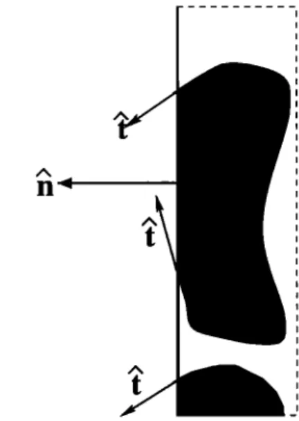
Figure 2. Side view of a cross section of a segment of the mixture adjacent to the surface of a control volume (as shown in Figure 1); the solid line on the left of the rectan- gular sample shows the surface boundary, while the dashed boundaries indicate that the sample is connected to the rest

of the volume. Black and white material is the same as in

Figure 1; that is, they represent either fluid or matrix. The unit tangents to the interface (at the intersection with the sur-

face

of the control

volume)

• and

unit

normal

to the surface

of the control volume fi are illustrated; see text surrounding (25) and (26).

which differs from surface free energy (denoted by •ci in sec- tion 5 and Appendix A2), Ci is the curve which traces the

intersection between the interface and the surface of the con-

trol volume (see Figure 1), dœ is a line element along Ci, and

• is a unit vector that is both normal to the line element dœ

and tangent to the interface (Figure 2 )[see also Drew and Segel, 1971]. However, we seek the effective surface ten- sion force acting on an element of surface area dA (a small segment of 5A); the element dA itself contains the intersec- tion curve ci, which is a small portion of Ci. As shown in

Appendix

A1,

we

can,

with

isotropy,

replace

fc•

•dœ

with

aafidA, where cr is a reduced surface tension (the reduction

is typically O(1); see Appendix A1). Thus summing over all area elements on 5A, the net surface tension force per unit

volume

becomes

(1/SV)

f•A ac•fidA,

in which

case

the

net

force equation assumes the form

0 - -X7P + X7. •_- pg• + X7(aa). (26) The last term in (26) is an effective surface tension body

force on the total mixture. (If we were to allow for anisotropy,

then

fc•

• dœ

would

be

most

likely

related

to a•_.

fidA,

in

a term proportional to X7 ß (aa); see also Drew and Segel

[1971].)

The force equations for each phase, (23) and (24), must sum to equal (26), indicating that

[see also Drew and Segel [1971]. Equation (27) might be easily misconstrued as a stress jump condition since it ap- pears similar to the jump condition for the interface between

two fluids with surface tension [Landau and Lifshitz, 1987;

Leal, 1992]. Such a jump condition is required at an internal boundary whose shape, location, and orientiation are known and that separates two adjacent but distinct fluid volumes that do not individually fill the entire domain. Given the continuum approach of two-phase theory, however, the spe- cific location and orientation of the interface are unknown; the interface as well as the two phases are treated as contin- uous quantities that exist at all points in the domain. (Even if anisotropy is allowed, the tensor a_q_ gives only the average

orientation of fabric due to the interface but not the loca-

tion and orientation of the interface itself.) Thus the two-

phase equations do not require an internal boundary condi- tion, and the inappropriate imposition of such a condition would lead to an overdetermined problem. Therefore (27) does not indicate that there is a jump in the interaction forces

but rather that the interaction forces themselves each con-

tain some component of the surface tension force. Since surface tension acts through the common interface between fluid and matrix, then the volume-averaged, effective body force X7 (orca) acts equally on equal-sized particles of fluid or

matrix (i.e., it does not act differently on the two phases as

does, say, the gravitational body force); we thus assume that at any point (or infinitesimal volume) in the mixture a frac- tion q• of this force acts on the fluid, while a fraction 1 - q•

acts on the matrix. We therefore write

hf = n + q•v'

(orca)

(28)

h,• = -n + (1 - ½) v (ac•) (29)

where r/is the component of the interaction forces that act equally and oppositely to each other; (28) and (29) automat-

ically satisfy (27).

The force r/has few constraints. By material invariance, r/has to be a function of vector variables that are antisym- metric to a switch of the subscripts f and m, such as Av and X7q•. Moreover, r/must account for (1) the viscous in-

teraction due to relative motion between the fluid and ma-

trix and (2) pressure acting at the interface. The simplest viscous interaction force that preserves Galilean invariance

(frame independence) is c(vm - v f) -- cAv, where c is a

scalar to be discussed further below [Drew and Segel, 1971; McKenzie, 1984]. The pressure contribution to the interfa- cial force must allow for equilibrium (no motion) when pres- sure is constant everywhere; for example, at least a portion of this force must cancel the part of the pressure force term

in (23) that goes as -Pf Vq3 (and similarly for (24)). There- fore the most basic form of the interface force is

r/- cAv + P*X7q•, (30) where P* is some averaged pressure that must be the same in each phase and is invariant to a switch of f and m. In

general, we write P* - •/Pf + (1 - ')')Pro, where '), is some

unknown weighting that is _< 1 and that, like q•, switches

to 1 - 3' if f and m are switched. (Note that in writing

P* as a function of Pf and Pro, we assume that the interfa-

cial average pressures are linearly dependent on the average

pressures in each phase; see Drew and Passman [ 1999] for a

discussion of interfacial pressure.) Also, if the system were

anisotropic, the relation for r/would need to be adjusted; see the comment at the end of section 4.3.

It is important to recognize that r/represents the equal and opposite force of one phase against the other, not the force of either phase against surface tension on the interface. In

fact, one can see by (26) that all the other forces involving

VP and V ß •, etc. work against the surface tension force V(cra). (Indeed, the correct stress jump condition arises from integrating (26) about a vanishingly thin volume cen-

tered on the interface, accounting for that the fact that a be-

comes a Dirac r5 function centered on the interface (see (5)),

not by integrating (27) about the interface.) Thus the forces

hf and

hm include

surface

tension,

while

all the other

forces

potentially balance surface tension. Therefore, upon substituting

hf = cAv + ['7Pf

+ (1 - 9')Pm]Vq•

+ q•V(aa) (31)

h,• =-cAv-['yPf+(1-3`)P,•]Vcg+(1-c))V(aa)

(32)

into (23) and (24), we obtain (after some rearrangement)

o = -

[vP +

+ v ß

+ cAv + (1 - 7)APVq• + q•V(aa) (33)

0 = - (1 - q•)[VP,• + p,•!/i] + V. [(1 - q•)r__,•]

- cAv + 9,/XPVq• + (1 - q•)V(aa) (34)

We can estimate 9' by considering the conditions for no motion; this requires zero velocities, zero nonhydrostatic pressure gradients, zero viscous stresses, and a constant cr (since a gradient in surface tension in a viscous medium can only be balanced by viscous stresses; see Landau and Lif-

shitz, 1987; Leal, 1992). In this case, (33) and (34) become

(1 - 7)APVq• + q•crVa = 0 (35) -7APVq• + (1 - q•)crVc• = 0, (36) which can only both be true if

On

the

assumption

that

7 - 1 - ½ for

aI

} situations

our

o = -

[vP +

+ v ß

+ c•v + O [•PVO + V(aa)] (37)

0 - - (1 - qS)[VPm

+ ping

•'1

+ V' [(1 - qS)Zm]

- cAv + (1 - qS)[APVq5

+ V(ac•)].

The force equations in the form of (37) and (38) are by no means complete since there are various issues that remain to be developed, such as the nature of the surface tension force, the form of the volume-averaged viscous stresses

and *'m, the meaning

of c, etc. We will deal with these

se-

8894 BERCOVICI ET AL.: TWO-PHASE COMPACTION AND DAMAGE, 1, THEORY

4.1. Surface Tension Force and Interface Equilibrium As discussed in section 2.2 the interface area density a is

assumed a function of •b wherein da/dck is the sum of av-

erage interface curvatures. With this assumption the surface

tension body force in (26) becomes

da

V(aa)

- a•V•b

+ aver.

(39)

The first term on the right-hand side of (39) represents the

surface tension force due to interface curvature, while the

second term is a force due to gradients in cr itself which result from temperature fluctuations (or gradients in surfac- tants; Landau and Lifshitz, 1987; Leal, 1992). Gradients in

yield effects such as Marangoni convection wherein temper-

ature anomalies in an exposed, thin fluid layer cause imbal- ances in surface tension at the layer's free boundary which in turn drive motion (see review by Berg et al. [ 1966]).

In the case of no motion, as in (35) or (36) using '7 = 1-(b, there can be no gradient in cr (which can only be balanced by

viscous stresses in a fluid [Landau and Lifshitz, 1987; Leal, 1992]), and the force equations yield the equilibrium surface tension (Laplace's) condition (assuming the force balance holds for all

da

Pt - Pm = rr• (40) (see also Appendix A2). However, we must emphasize this

condition is only true when the system is static or quasi- static, adiabatic, and in equilibrium; a more general condi-

tion will be explored in section 5. 4.2. Average Viscous Stress Tensors

To obtain a closed theory, it is necessary to express the

average

viscous

stress

tensors

T_f and

Zm in terms

of aver-

age velocities vf and vm. While the assumption that these stresses obey the constitutive laws for single-phase media

[e.g., Loper and Roberts, 1978; McKenzie, 1984; Loper,

1992] is somewhat ad hoc, we can provide some constraints which partially justify such an approach.

By our definition of volume averaging, the average vis-

cous

fluid

stress

r_f is given

by

1 f• (V•/+

[V•/]

t)

OdV

(41)

given that pf is assumed constant. Derivation of the relation

between

Zf and

vf requires

an evaluation

of the integral

of

the true velocity gradients; by considering one gradient term

we can write (again given the same assumptions associated

with (11 ))

1 f• (X7•,f)OdV_

1 fa [X7(Ogf)-(VO)•'f]dV

5V • 5V •

1 f• (VO)•rfdV.

(42)

= V(0vi)

- -ff v

The other velocity gradient term can be treated identically,

leading to

c•Zf

-- pf {V(oSvf)

+ [V(oSvf)]

t - (U l + IJ})}, (43)

where

1 f• (VO)•rfdV.

(44)

Es=aft v

The tensor

U__f

contains

bulk

information

about

the fluid

ve-

locity at the interface; its evaluation is by no means trivial and has been given a variety of treatments [Ganesan and

Poirier,

1990;

Ni and

Beckerman,

1991

]. Although

Uf can-

not be solved exactly in terms of average velocities, there are several fundamental constraints that can help us estimate its

form:

1. [If must

contain

a term

to insure

that

the stress

tensor

T_f is Galilean

invariant.

In particular,

it must

have

a part

that depends on (V 4)uf, where uf is some as yet undefined

velocity; in this case, the stress terms dependent on velocity

in (43) will appear as (V•5)(vf - uf) thereby removing the

velocity of the frame of reference.

2. The trace

of Uf is given

by (18) and

thus

Tr(Ui) = •bV.v I + v I ß V•b.

(45)

3. The whole

stress

tensor

Zi itself

must

have

zero

trace;

that is, it remains the deviatoric stress even after volume av-

eraging. This is required because regardless of how we do any volume averaging, the fluid and matrix are always in- compressible, and thus when the mixture is exposed to a uni- form isotropic stress, it should not undergo compression and only its pressure should increase.

4. Since

U.i is linear

in • and

0, it is reasonable

to expect

that it be linear in vi and •b (as also suggested by (45)).

5. U__i

must

contain

unique

terms;

that is, it cannot

only

be made up of terms that merely cancel all of V (•bvi), thus

leading

to a null stress

tensor

Zi. In other

words,

although

U__i

= V (•bvi) would

satisfy

all the previous

constraints,

it

would

also

lead

to Zi = 0, which

is unacceptable.

6. Finally,

any stress

tensor

Zi resulting

from

the choice

of U__i

must

have

a positive

definite

contribution

to the

dissi-

pation

function,

i.e., Vvi: Zi _• 0, in order

to satisfy

the

second law of thermodynamics; see section 5 for discussion of dissipation.

The simplest

(but

by no means

unique)

form

of U__i

that

satisfies these six basic constraints is

U

i - (V4)v/+

•4V.

vii.

(46)

This leads to a stress tensor given by

•T---f

--

•tZ

f ( vv

f + [vv

f ]t 2 0

-õV.vs ,

(47)

which is, of course, the simple deviator for nonsolenoidal velocity fields and is thus intuitively appealing. By similar arguments, and by symmetry, we arrive at the relation for the

average matrix stress tensor

(

,

i_)

(1--•))T'

m

-- (1--•))•m

VYm

-• [VYm]

t -- •V'¾m ß

Neither (47) nor (48) explicitly contain the bulk viscosity term used by McKenzie [1984] since we have precluded compression under a uniform isotropic stress. However,

isotropic compaction is allowable if the two phases expe-

rience different isotropic stresses; for example, the matrix

is isotropically loaded but the fluid is left free to escape (D.

McKenzie, personal communication, 2000); as discussed in

section 5 (see the explanation surrounding (68)), this pro-

cess is treated through the pressure difference Ap instead

of through a bulk viscosity effect.

The constitutive laws (47) and (48) are somewhat simpler than those arrived at by various workers [Ishii, 1975; Ni and Beckerman, 1991] and not very different from what others

[Loper and Roberts, 1978; McKenzie, 1984] have assumed

would be the constitutive laws. However, while (47) and (48) are not derived uniquely, they are arrived at more rigorously than usual, and their deduction from the above considera-

tions partially justifies their simple form. Finally, we briefly

note that if we were to consider anisotropy it undoubtedly

occurs

in the tensor

Uf (and its matrix

counterpart)

as it

derives from integrals of the quantity •70; we would thus

assume

that

an anisotropic

version

of Uf would

involve

c•,

thereby leading to an anisotropic stress tensor. 4.3. Interaction Coefficient c and Darcy's Law

The fluid force equation (37) reduces to something similar

to Darcy's

law when

Zf (or more

precisely/•f)

is negligible

and APV•b+ V(act) = 0 (implying that either the pressure

drop balances surface tension or that surface tension and the pressure drop are both zero), i.e.,

C(Vf -- Vm) = -qb(VPf q- pfg9•)

(49)

[see also McKenzie, 1984]. If there is sufficient interconnect-

edness of pores, (49) suggests that the coefficient c should be related to the permeability of the matrix and the viscos-

ity of the fluid,

i.e., c = I•fqb2/k,

where

the permeability

k

is a function of porosity •b [McKenzie, 1984; Ganesan and Poirier, 1990]. However, this relation for c cannot be used generally (i.e., for arbitrary viscosities) since it would violate

material invariance (i.e., symmetry to a switch of subscripts

m and f) of the force equations (37) and (38). We can es-

timate a more general expression for c by considering the

balance of viscous forces at the fluid-matrix interface. We assume that (1) the forces represented by cAv arise from viscous deformation at the pore and grain scale, i.e., due

to deformation of fluid or matrix within the pore or grain;

(2) the scales for the viscous force per volume in the two phases have similar forms; and (3) these forces match at the

interface. These assumptions lead to a relationship between viscous force scales:

V m -- V i V i -- Vf

,

(50)

where vi is the interface velocity and 6; is the typical size

of an element of phase j (meaning a fluid pore if j - f and

terms of vf and vm, we can estimate the viscous force scale (either side of (50)) and equate it to the interface force on the fluid, leading to

C(V

m

-- Vf)

-- ]gmIgf(Vm

_I•f62•

_{+ 1•,•6•}

-- Vf)

_'

₍₅₁₎

If we assume that 6f and 6m are related to permeability k

and (like permeability) me assumed to be functions only of porosity ½, then to preserve symmetry of the equations (ma-

terial invariance), they must be related to the same function of porosity, i.e.,

6f =6(0) 6• = 6(1 - O). (52)

If we wish to recover Darcy's law, then in the limit •f (( •m

we obtain

lim c- /•f(/)2 /•f

(53)

which

implies

we would

use

5(•b) - V/•(•b)/•b.

As ex-

pected, permeability is related to pore and/or grain size and thus contains information about the mixture's fabric; there- fore k is necessarily also related to the interface density a (see section 2.2). If pore and grain sizes are uniquely repre- sented by permeability, then a general form of c is

•m•f•b2(1 -- •b)

2

c --

02 k(•b)(1

0)

2' (54)

which has the proper symmetry.

The dependence of permeability on porosity has vari- ous forms [Bear, 1988; Furbish, 1997], although these are largely based on empirical estimates in which the matrix is

immobile (/•,• >> /•). For small porosities one often uses the simple model k(•b) - koc) n [see Spiegelman, 1993c, and

references therein]. If there is not sufficient interconnected-

ness of pores and/• is not <</•m, then use of Darcy's law

as a constraint is not valid, although a relation of the form

given in (5 l) is probably still general enough to even cap- ture relative motion of isolated bubbles in a matrix [e.g., see

Batchelor, 1967].

Regardless of whether or not we use permeability and

Darcy's law, it is clear that c depends on grain and/or pore size and thus should be related to the interface area density a (see section 2.2). Thus, if the system were anisotropic, we would likely replace c with a tensor c_ that is related to •, and the interaction force cAv would be replaced by c_. Av; by the same token, an anisotropic permeability also should be determined by •. Moreover, the part of the force r/that

represents a pressure acting on the interface (see (30)) would

likely be proportional to V .• instead of V•b.

5. Energy Conservation, Surface Energy, and

Damage

So far, we have derived eight conservation equations: two continuity equations (12) and (13) (or alternatively (15) and

a matrix

grain

if j - m). (Equation

(50) accounts

for the (16)) from

conservation

of mass

and

six force

equations

(37)

fact that as in simple shear across a boundary, if v,• > vi, and (38). However, even without anisotropy, this system is

8896 BERCOVICI ET AL.' TWO-PHASE COMPACTION AND DAMAGE, 1, THEORY

ity ½, six velocities vf and v,• (or alternatively V and Av),

and

two

pressures

Pf and

Pm (or alternatively

P and

Ap).

only valid for zero or weak motion and assumes conditions

of thermodynamic equilibrium and isentropy (see Appendix A2), which are not general conditions and are inappropriate for problems involving large viscous forces and/or rapidly deforming systems. To incorporate deformation and viscous stress, it is tempting to posit a vector jump condition on total

stress such as AZ. X7c) - APVq5 -- V(aa), which would

be analogous to an interface condition [Landau and Lifshitz, 1987; Leal, 1992] in which V ½ serves as crude proxy for the

unit normal to the interface. However, as stated earlier, such

conditions would be valid only if the interface were well de- lineated and thus required a boundary condition across it. With the averaging implicit in a mixture theory the interface is not delineated; it is, instead, mathematically treated as a continuous quantity that exists at all points in the domain with a particular concentration (in this case, area per volume a); thus a vector jump condition would be inappropriate and would impose an overdeterminedness on the system.

Perhaps the simplest relation for Ap, the equilibrium sur- face tension condition (40), is generally derived from ba- sic thermodynamics (i.e., conservation of energy assuming equilibrium, or minimum energy, and isentropic conditions [Landau and Lifshitz, 1987; Bailyn, 1994]); see Appendix A2. In this section we attempt to infer a ninth equation to ef- fectively constrain AP from a more general thermodynamic approach, i.e., conservation of energy far from equilibrium and with entropy production.

Our basic energy conservation law differs little conceptu- ally from that derived previously [McKenzie, 1984; Poirier et al., 1991]; the time rate of change of internal energy within a control volume •V is governed by (1) the rate of loss of this energy through the surface of the volume via both mass transport and diffusion; (2) the rate at which work is done on the volume by the net surface and body forces; and (3) the rate of internal energy or heat production. In our system, however, the internal energy contained within •V exists in not two but three phases, i.e., the fluid and matrix phases and the interface. We will first write down the energy conservation law and then discuss the various assumptions

that have gone into it. If sf and Sm are the internal energy

per unit mass of the fluid and matrix phases, respectively (averaged over the volumes of their respective phases) and •i is the energy per unit of interface area (averaged over a small volume of the mixture), then the rate of energy change per volume is given by

o[

]

0-• •Sp•e•

+ (1 - •)Pmem

+ •iOz

-- Q - V.q

-- V ' (•pf•fVf -•- (1 - •)PmSmV m + •iO• r) + V. (-OvIPI -(1- O)vmPm

+ •Sv• 'r_• + (1 - •5)Vm-r

m + Vac•)

-- qSvf. (pfg•) -- (1 - •p)v m ß (pmg•), (55)

where Q is the inherent rate of energy (heat) production per unit volume, q is the diffusive energy flux vector (e.g., the heat flow vector). The second term on the right of (55) rep- resents the rate of energy transport across the surface of the volume (Figure 1), the third term represents the rate at which work is done by surface forces on the surface of the volume, and the last two terms represent the rate at which work is done by the body forces on the interior of the volume. As basic as this equation appears, several implicit assumptions necessary for its derivation should be discussed:

1. As appropriate for our creeping flow system, changes in kinetic energy are neglected [see also McKenzie, 1984].

2. In (55) the nonlinear products between various depen- dent quantities (in particular, velocity with energy, pressure, or stress) appear to be represented only with the products of the volume-averaged quantities. This representation is not entirely accurate and therefore warrants some discussion. In

particular,

say

we have

two

true

fluid

quantities

.• and

•,

and their averages A and B are defined in the standard way,

e.g.,

qSA

- (1/SV)

far •OdV.

Then

we

can

also

write

that

A - A + A • and/• - B + B •, where

the averages

of the

perturbations A • and B • are zero. The volume average of the

product

A and/• differs

from

the

product

of A and

B, i.e.,

f6 --

1 f, A'

B'

OdV.

1 ABOdV

- c)AB

+ •-• v

5V v (56)

The evaluation of the last term on the right is, of course, a classic problem in turbulence mean field and closure theo- ries. In problems of heat and chemical transport in porous media this term is typically parameterized into a quantity called dispersion, which mathematically looks very much like diffusion [Bear, 1988; Furbish, 1997]. While this type of dispersive transport might be a reasonable representa- tion of the bulk transport terms, i.e., the nonlinear prod- ucts between velocities and internal energies, it is possibly less justified for the products between velocities and stresses or pressures. A rigorous estimate of these nonlinear terms invariably requires higher-order closure theories, introduc- ing yet more equations and unknowns. While this problem might prove fruitful in future studies, we presently opt to maintain the maximum level of simplicity. We thus assume that the nonlinear terms in question are zero (meaning es- sentially a zero correlation between the quantities A • and

B •, regardless of what these quantities are) or that they can

be deemed a form of dispersion and thus absorbed into the quantity q (thus q would not necessarily represent only heat flow). Neither assumption is completely satisfactory, yet the

alternatives are less so.

3. As discussed in section 4, surface tension, when aver- aged over an area element on the surface of a control volume, exerts a force per area ac•fi (where fi is the unit normal of

the area element). Since this effective averaged force acts

equally on particles of matrix and fluid (given that it actu- ally acts through their common interface) we assume that a

fraction ½ of it acts on fluid which moves at velocity v f,

while a fraction 1 - ½ acts on matrix which moves at ve- locity Vm. Thus the net rate of work done (per area) on material at the surface by surface tension is assumed to be