HAL Id: insu-03025061
https://hal-insu.archives-ouvertes.fr/insu-03025061
Submitted on 26 Nov 2020
HAL is a multi-disciplinary open access
archive for the deposit and dissemination of
sci-entific research documents, whether they are
pub-lished or not. The documents may come from
teaching and research institutions in France or
abroad, or from public or private research centers.
L’archive ouverte pluridisciplinaire HAL, est
destinée au dépôt et à la diffusion de documents
scientifiques de niveau recherche, publiés ou non,
émanant des établissements d’enseignement et de
recherche français ou étrangers, des laboratoires
publics ou privés.
Eunok Yim, P. Billant, F. Gallaire
To cite this version:
Eunok Yim, P. Billant, F. Gallaire. Nonlinear evolution of the centrifugal instability using a semi-linear
model. Journal of Fluid Mechanics, Cambridge University Press (CUP), 2020. �insu-03025061�
For Peer Review
This draft was prepared using the LaTeX style file belonging to the Journal of Fluid Mechanics 1
Nonlinear evolution of the centrifugal
instability using a semi-linear model
Eunok Yim
1†, P. Billant
2and F. Gallaire
11LFMI, ´Ecole Polytechnique F´ed´erale de Lausanne, 1015 Lausanne,Switzerland 2LadHyX, CNRS, ´Ecole Polytechnique, F-91128 Palaiseau CEDEX, France
(Received xx; revised xx; accepted xx)
We study the nonlinear evolution of the axisymmetric centrifugal instability developing on a columnar anticyclone with a Gaussian angular velocity using a semi-linear approach. The model consists in two coupled equations: one for the linear evolution of the most unstable perturbation on the axially averaged mean flow and another for the evolution of the mean flow under the e↵ect of the axially averaged Reynolds stresses due to the perturbation. Such model is similar to the self-consistent model of Mantiˇc-Lugo et al. (2014) except that the time averaging is replaced by a spatial averaging. The non-linear evolutions of the mean flow and the perturbations predicted by this semi-linear model are in very good agreement with DNS for the Rossby number Ro = 4 and both values of the Reynolds numbers investigated: Re = 800 and 2000 (based on the initial maximum angular velocity and radius of the vortex). An improved model taking into account the second harmonic perturbations is also considered. The results show that the angular momentum of the mean flow is homogenized towards a centrifugally stable profile via the action of the Reynolds stresses of the fluctuations. The final velocity profile predicted by Kloosterziel et al. (2007) in the inviscid limit is extended to finite high Reynolds numbers. It is in good agreement with the numerical simulations.
Key words: Centrifugal instability, vortex, semi-linear model, stability analysis
1. Introduction
Centrifugal instability or inertial instability, is the most common instability developing on vortices in rotating medium. It is a local instability occurring when the balance between the centrifugal force and the pressure gradient is disrupted, i.e. when the square of the absolute angular momentum of the fluid decreases with radius r in inviscid fluids (Rayleigh 1917; Synge 1933; Kloosterziel & van Heijst 1991). While this condition applies to axisymmetric disturbances, a generalized criterion for non-axisymmetric perturbations has been derived by Billant & Gallaire (2005).
Linear stability analysis of a columnar vortex with Gaussian angular velocity in inviscid fluids shows that the growth rate is maximum at infinite wavenumber (Smyth & McWilliams 1998). However, as soon as viscous e↵ects are taken into account, short wavelength are damped and the fastest growing mode has a finite wavenumber (Lazar et al. 2013; Yim et al. 2016).
Kloosterziel et al. (2007) and Carnevale et al. (2011) have analysed the nonlinear
For Peer Review
evolution of the centrifugal instability in a rotating medium at high Reynolds number. They have shown that the vortex saturates to a centrifugally stable state where the Rayleigh instability condition is no longer satisfied, i.e. the square of the axial average of the absolute angular momentum does not decrease with radius. Hence, the instability redistributes the regions of positive and negative absolute angular momentum under the constraint of absolute angular momentum conservation in the inviscid limit.
The saturation of an instability towards a periodic limit cycle for which the mean flow is stable has been recently described by means of a self-consistent approach (Mantiˇc-Lugo et al. 2014). In this approach, the flow is decomposed into time-averaged mean flow and unsteady perturbations. Then, the nonlinear saturation can be described by computing the mean flow distortion due to the Reynolds stresses of the perturbation and the linear growth of the perturbation on the mean flow. Here, we develop a similar approach for the centrifugal instability using a spatial average instead of a time average since the instability is spatially periodic but not periodic in time.
2. Governing equations
We consider the Carton & McWilliams vortex (Carton et al. 1989) with angular velocity (figure 1a)
⌦ = ⌦0exp( r2/R2), (2.1)
where ⌦0 is the maximum angular velocity and R the radius of the vortex. Such isolated
profile is frequently observed (Ioannou et al. 2017) and its stability has been extensively studied (Carton et al. 1989; Gent & McWilliams 1986; Smyth & McWilliams 1998; Billant & Gallaire 2005; Kloosterziel et al. 2007; Yim & Billant 2015). The vortex (2.1) is a steady solution of the Euler equation since it is axisymmetric and axially uniform. It is also an exact solution of the Navier-Stokes equation when ⌦0 and R are allowed to vary with
time as follows: ⌦0= ⌦i(Ri/R)4 with R2= R2i+ 4⌫t, where ⌫ is the kinematic viscosity
and ⌦i, Ri are the initial angular velocity and radius. In the following, the length and
time are non-dimensionalised with R and 1/⌦0, respectively. The governing equations
for the velocity field u = [u, v, w] in cylindrical coordinates (r, ✓, z) read @u
@t + u· ru + 2Ro
1e
z⇥ u = rp + Re 1r2u, (2.2)
r · u = 0, (2.3) where the Reynolds and Rossby numbers are defined as Re = ⌦0R2/⌫ and Ro = 2⌦0/f ,
respectively with f the Coriolis parameter. The divergence free condition (2.3) is not further written in the following sections but is always guaranteed.
2.1. Linear stability
The linear stability of the base flow (2.1) has been first studied by linearizing the equations (2.2)–(2.3) and assuming infinitesimal perturbations with axial wavenumber k, azimuthal wavenumber m and growth rate
[˜u, ˜p](r, ✓, z, t) = [u, p](r)e t+ikz+im✓+ c.c., (2.4) where c.c indicates the complex conjugate and giving
u +Lm,k(ub)u = 0, (2.5)
where
Lm,k(ub)u⌘ ub· rm,ku + u· rub+ 2Ro 1ez⇥ u + rm,kp Re 1r2m,ku, (2.6) Cambridge University Press
For Peer Review
Nonlinear evolution of the centrifugal instability using a semi-linear model 3
(a) 0 1 2 3 0 1 2 r ⌦ , ⇣ ⌦ ⇣ (b) 0 10 20 0 0.1 0.2 0.3 kz Re = 800 Re = 2000 (c) 0 1 2 2 1 0 1 r u Im(u) Im(v) Re(w)
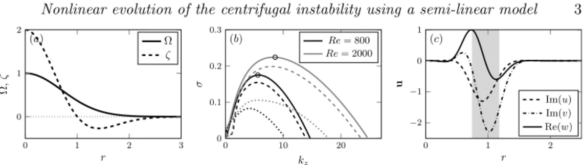
Figure 1. (a) Angular velocity (⌦) and axial vorticity (⇣) of the base flow. (b) Linear growth rate as a function of the vertical wavenumber k for di↵erent azimuthal wavenumbers: m = 0(solid lines), m = 1(dashed lines), m = 2(dotted lines) for Re = 800(black lines) and Re = 2000(grey lines) for Ro = 4 The circles indicate the most unstable modes. (c) Most unstable eigenmode for Re = 800. The shaded area indicates the region where < 0.
where ub= [0, r⌦, 0]. Here, rm,k andr2m,k are respectively the gradient and Laplacian
in cylindrical coordinates with the azimuthal derivative replaced by im and the vertical derivative by ik.
In the inviscid limit, the necessary and sufficient condition for the instability of axisymmetric perturbations reads (Rayleigh 1917; Synge 1933; Kloosterziel & van Heijst 1991), = 2 ✓ v r + 1 Ro ◆ ✓ ⇣ + 2 Ro ◆ < 0. (2.7) For the base flow (2.1), (2.7) is satisfied when Ro < 1 or Ro > exp(2). Figure 1b shows the linear growth rate as a function of k for di↵erent azimuthal wavenumbers m for Ro = 4 for two di↵erent Reynolds numbers, Re = 800 and Re = 2000. The growth rate is maximum for the axisymmetric mode at km = 5.6 for Re = 800 and
km= 8.6 for Re = 2000. As predicted by the generalized criterion of Billant & Gallaire
(2005), only the first nonaxisymmetric modes m = 1 and m = 2 are unstable and their maximum growth rate is lower than for m = 0. Hence, in the following, we will focus on the axisymmetric mode at the most amplified vertical wavenumber km. Figure 1c shows
the most unstable eigenmode for Re = 800, Ro = 4. It is mostly localized in the region where the Rayleigh discriminant is negative (shaded area).
3. Semi-linear formulation
We decompose the flow as
u(r, ✓, z, t) = u(r, ✓, t) + ˆu(r, ✓, z, t), (3.1) where u = z 1
max
Rzmax
0 udz is the axially averaged mean flow and ˆu the perturbation which
is not assumed to be small as in the linear stability analysis. Averaging the equation (2.2) in z leads to
@u
@t + u· ru + 2Ro
1e
z⇥ u + rp Re 1r2u = uˆ· rˆu. (3.2)
Substracting (3.2) from (2.2) yields the equation for the perturbation ˆu, @ ˆu
@t + u· rˆu + ˆu · ru + 2Ro
1e
z⇥ ˆu + rˆp Re 1r2u =ˆ uˆ· rˆu + ˆu · rˆu. (3.3)
These mean and fluctuation equations are similar to those of the Reynolds decomposition (Reynolds & Hussain 1972). They involve several coupling terms between the mean
For Peer Review
and the fluctuation. The right hand side of (3.2) is the Reynolds stress due to the fluctuations which acts as forcing or added momentum to the nonlinear mean flow equation (left hand side of (3.2). The amplitude of this forcing is proportional to the square of the fluctuation amplitude. In turn,the fluctuation in (3.3) is a↵ected by the evolution of the mean flow through the advection operator (u· rˆu + ˆu · ru). The fluctuation evolves also due to nonlinear e↵ects with zero mean (right-hand side of 3.3) (Mantiˇc-Lugo et al. (2014, 2015)).
3.1. Single harmonic
We introduce now the normal mode form of the perturbation for m = 0: ˆu(r, ✓, z, t)⌘ ˆ
u(r, z, t)' u1(r, t)exp(ikmz) + c.c. where kmis the most amplified wavenumber obtained
from the linear stability analysis. At t = 0, the perturbation is set as u1(r, 0) = A0um
where um is the dominant eigenmode and A0 the initial amplitude of the perturbation.
Neglecting the higher harmonics, the governing equations (3.2)-(3.3) reduce to @u @t + u· ru + 2Ro 1e z⇥ u + rp Re 1r2u = ⇠(u1), (3.4) @u1 @t +L0,k(u)u1= 0, (3.5) whereL0,k(u) is a linear operator defined in (2.6) with m = 0 and ⇠(u1) = u1· r ku⇤1+
u⇤
1· rku1 is the Reynolds stress. It is worth mentioning that (3.4) – (3.5) are now only
a function of time and the radial coordinate r. In addition, the divergence free condition reduces to 1/r@ru/@r = 0 since @w/@z = 0 due to the axial averaging. This implies u = 0. It can also be shown that w remains identically zero for all time if w = 0 at t = 0, since the Reynolds stress in the z direction is zero. Thus, the mean flow has only a component along the azimutal direction u = [0, v, 0]T. Hence, (3.4) simplifies to
@v @t = Re 1 @2v @r2 + 1 r @v @r v r2 ⇠(u1)✓, (3.6)
which is a simple di↵usion equation with a source term independent from the Rossby number Ro. Using the axisymmetry of the mean flow and of the perturbation, the linear equation (3.5) can be also further reduced to
@⌘1 @t ✓ 2v r + 2Ro 1 ◆ ikv1 Re 1 @2⌘ 1 @r2 + 1 r @⌘1 @r ⌘1 r2 k 2⌘ 1 = 0, (3.7a) @v1 @t + ⇣ + 2Ro 1 u 1 Re 1 @2v 1 @r2 + 1 r @v1 @r v1 r2 k 2v 1 = 0, (3.7b)
where ⌘1 = @zu1 @rw1= iku1 (i/kr)@r((1/r)@rru1) is the azimuthal component of
vorticity.
Therefore, our model consists in the semi-linear 1D equation (3.5), or equivalently (3.7), for the evolution of the perturbation over the mean flow coupled to the equation (3.6) for the evolution of the mean flow under the e↵ects of the Reynolds stresses of the perturbation and viscous di↵usion. The only di↵erence compared to pure linear equations is this evolution of the mean flow. Such semi-linear model is similar to the self-consistent model proposed by Mantiˇc-Lugo et al. (2014). The main di↵erence is that the Reynolds decomposition (Reynolds & Hussain 1972) to separate the flow into a mean flow and a fluctuation is here based on spatial axial average since the perturbation is harmonic along the axis while the self-consistent model relies upon a time average because the perturbation is harmonic in time for the flows they have considered. Another di↵erence
For Peer Review
Nonlinear evolution of the centrifugal instability using a semi-linear model 5 is that the perturbation equations are here simply integrated in time while, in the self-consistent model, an eigenvalue problem has to be solved after each variation of the mean flow.
3.2. Two harmonics
One can easily include higher harmonics of the fundamental mode following the same approach. For instance, taking into account the second harmonic in the velocity perturbation: ˆu = u1(r)exp(ikmz) + u2(r)exp(i2kmz) + c.c., the perturbation equations
become @u1 @t +L0,k(u)u1= (u2· r ku ⇤ 1+ u⇤1· r2ku2), (3.8a) @u2 @t +L0,2k(u)u2= (u1· rku1). (3.8b) The mean flow (3.6) is then forced by the Reynolds stress of both harmonics
@v @t = Re 1@2v @r2 + 1 r @v @r v r2 ⇠(u1)✓ ⇠(u2)✓. (3.9)
Higher harmonics 3km, 4km,· · · can be taken into account similarly. Since the
per-turbations equation are integrated in time, there is no particular complexity arising when several harmonics are considered. This is in contrast with the self-consistent model (Mantiˇc-Lugo et al. 2014) where the eigenvalue problems become increasingly complicated when more than one harmonic is considered (Meliga 2017).
3.3. Numerical method
The semi-linear numerical simulations have been performed with the FreeFEM++ software (Hecht 2012) for axisymmetric cylindrical coordinates (r, z). The velocity and pressure of equations (2.2)–(2.3) are discretised with Taylor-Hood P2 and P1 elements, respectively. The time is discretised using the first order backward Euler formula. The total numbers of degree of freedom is 4687. Three-dimensional (3D) DNS have been performed using the open source spectral element code Nek5000 (Fischer et al. 2008) in Cartesian coordinates (x, y, z) in cylindrical geometry. The domain is discretized by 120000 hexahedral elements and each element is composed with 8 (velocity) or 6 (pressure) Gauss-Lobatto-Legendre quadrature points along each direction (resulting in 250 million degrees of freedom, i.e. 50000 times more than for the semi-linear models). The time and the nonlinear convection terms are discretised using third order backward di↵erentiation and third order explicit extrapolation formula, respectively.
Both DNS and semi-linear models are initialized with the perturbation ˆu = A0umexp(ikmz) + c.c. where A0 = 0.001 is the initial amplitude and um is the
most unstable linear eigenmode (figure 1c) obtained by means of the restarted Arnoldi method. The eigenmodes have been normalized so that the absolute maximum value of the vertical velocity is unity, max(|wm|) = 1 such that max(| ˆw|) = A0.
The domain size for the semi-linear model is chosen to be r = [0, rmax] where rmax= 8.
Since the base angular velocity decays exponentially with r2, the radial extent does not
need to be large: the eigenvalues and eigenvectors are converged as soon as rmax >
5. Periodic boundary conditions are applied on z = 0 and z = zmax. The boundary
conditions at r = 0 are u = v = 0 since the flow is axisymmetric (Batchelor & Gill 1962). At r = rmax, all perturbations are enforced to vanish. The domain sizes in the DNS are
r = [ 8, 8] along the horizontal with no slip boundary conditions and z = [0, 13· 2⇡/km]
For Peer Review
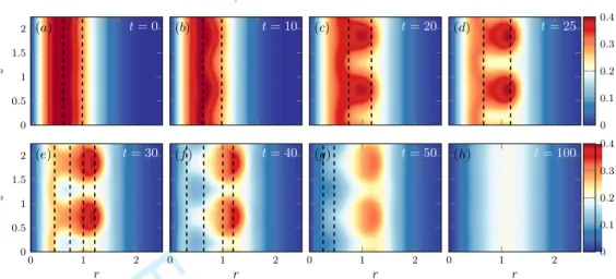
(a) t = 0 0 0.5 1 1.5 2 z (b) t = 10 (c) t = 20 (d) t = 25 0 0.1 0.2 0.3 0.4 (e) t = 30 0 1 2 0 0.5 1 1.5 2 r z (f ) t = 40 0 1 2 r (g) t = 50 0 1 2 r (h) t = 100 0 1 2 r 0 0.1 0.2 0.3 0.4Figure 2. Vertical cross-sections at x = 0 of the evolution of the azimuthal velocity field v in DNS for km= 5.6, Ro = 4, Re = 800. The dashed lines delimit the regions where ¯ < 0 based
on the mean azimuthal velocity ¯v. Only two wavelengths are shown whereas the full domain contains 13 wavelengths along the vertical (see§3.3).
some DNS and simulations with the semi-linear models have been also performed with an independent pseudo-spectral code NS3D (Deloncle et al. 2008). Identical results have been obtained.
4. Results
We consider a single Rossby number Ro = 4. This value has been chosen to be sufficiently far from the marginal stability limit Ro = 1 so that the initial growth rate and non-linear e↵ects are not weak. In other words, we are not in a weakly nonlinear regime as assumed to derive asymptotically amplitude equations. Two Reynolds numbers will be investigated: Re = 800 and Re = 2000 corresponding to di↵erent viscous damping and, thus, to di↵erent values of the initial growth rates (figure 1b). This allows us to test the semi-linear models for two representative cases where nonlinear e↵ects and higher harmonics are expected to be moderate (Re = 800) or more important (Re = 2000). Alternatively, di↵erent growth rates could have been obtained by varying Ro with Re fixed.
4.1. 3D DNS
Figure 2 shows snapshots of the azimuthal velocity v in a DNS for Ro = 4 and Re = 800. Only two wavelengths are displayed although the computation is performed over 13 wavelengths. The vertical lines delimit the regions where the Rayleigh discriminant ¯ is negative, where ¯ is based on the axially averaged azimuthal velocity ¯v(t, r). At t = 10, a slight deformation can be seen in the region where ¯ < 0. Subsequently, the perturbation grows and rearranges the distribution of azimuthal velocity (20 < t < 30). For t > 30, the ‘mushrooms’ start to fade out. Finally, vertical deformations are no longer visible by t = 100 so that the vortex then evolves only by viscous di↵usion.
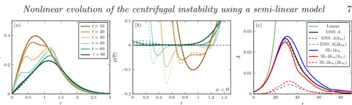
The solid lines in figure 3a show the evolution of the corresponding mean azimuthal velocity ¯v. The mean flow profile first decays by viscous di↵usion until t = 10. A distortion of the mean flow due to the instability can be seen at t = 20. At t = 30 and t = 40, it becomes strong and the profile exhibits two distinct peaks near r = 0.4 and r = 1. Then, the peak at r ⇠ 0.4 disappears and the mean azimuthal velocity profile becomes linear
For Peer Review
Nonlinear evolution of the centrifugal instability using a semi-linear model 7
(a) 0 0.5 1 1.5 2 2.5 3 0 0.2 0.4 r v t = 10 t = 20 t = 30 t = 40 t = 60 t = 80 (b) < 0 0 0.2 0.4 0.6 0.8 1 1.2 1.4 0.2 0.1 0 0.1 r (v ) (c) 0 20 40 60 80 0 0.01 0.02 0.03 t A Linear DNS A DNS A(km) DNS A(2km) SL-1km SL-2km(km) SL-2km(2km)
Figure 3. (a) Mean azimuthal velocity ¯v from DNS (solid lines) and SL-1km model (dashed
lines), (b) corresponding Rayleigh discriminant ¯ and (c) perturbation amplitudes A as a function of time for Ro = 4 and Re = 800.
for r < 1 for t > 60. During this process, the maximum velocity has decreased from max(¯v(t = 0)) = 0.47 to max(¯v(t = 80)) = 0.23 and the corresponding radius has moved from r = 0.7 to r = 1.2. The corresponding Rayleigh discriminant is shown in figure 3b (solid lines). At t = 0, ¯ is minimum at r = 0.95 and is negative for 0.75 < r < 1.18. For t = 20, the region where ¯ < 0 has enlarged but the minimum of ¯ has decreased in absolute value. At t = 30, there exist two regions where ¯ < 0: near r = 0.3 and r = 0.8 while ¯ > 0 in between. The minimum value decreases and then increases again for larger time. By comparing figure 3a and figure 3b, we can see that the mean flow is mostly deformed near the negative peaks of ¯ at least until t = 40. At t = 60, min( ¯) is no longer negative.
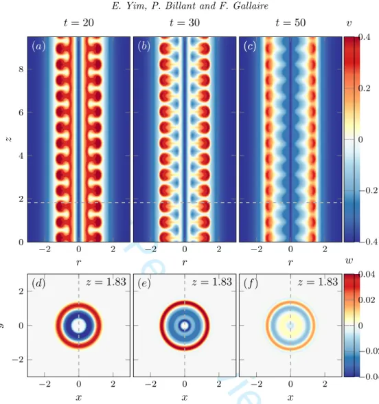
The evolution of the instability is qualitatively similar for the higher Reynolds number Re = 2000. (figure 4). For this DNS, full vertical cross-sections of the azimuthal velocity and horizontal cross-sections of the vertical velocity are displayed at three selected times. As can be seen, the flow seems to remain axisymmetric and no subharmonic modulations of the primary wavelength are visible along the vertical. This is confirmed quantitatively in figure 5a,b which shows the averaged azimuthal P✓(m, t) and axial Pz(k, t) Fourier
spectra defined as P✓(m, t) = 1 rmaxzmax Z rmax 0 Z zmax 0 F T✓[w(r, ✓, z, t)]F T✓⇤[w(r, ✓, z, t)]dzdr, (4.1) Pz(k, t) = 1 rmax Z rmax 0 F Tz[w(r, [0, ⇡], z, t)]F Tz⇤[w(r, [0, ⇡], z, t)]dr, (4.2)
where F T✓[w(r, ✓, z, t)] and F Tz[w(r, ✓, z, t)] are the azimuthal and axial Fourier
trans-forms of the axial velocity w. The axisymmetric m = 0 mode remains always largely dominant (figure 5a) and only the fundamental mode km and higher harmonics grows
significantly (figure 5b). This legitimates the assumptions behind the semi-linear models where only the most amplified axisymmetric mode, and possibly higher vertical harmon-ics, are taken into account.
The evolution of the mean azimuthal velocity ¯v for Re = 2000 (solid lines in figure 6a) resembles the one for the lower Reynolds Re = 800 (figure 3). The deformations at intermediate times are nevertheless more pronounced for Re = 2000.
4.2. SL-1km semi-linear model
The dashed lines in figure 3a represent the mean azimuthal flow predicted by the semi-linear model with one harmonic, abbreviated as SL-1km, for Re = 800. The agreement
with the DNS is almost perfect for t = 10, 20 while some discrepancies can be seen at t = 30, 40. It becomes excellent again for t > 60. Similar agreement and discrepancies are
For Peer Review
(a)
2 0 2 0 2 4 6 8r
z
t = 20
(b)
2 0 2r
t = 30
(c)
(c)
2 0 2r
t = 50
0.4 0.2 0 0.2 0.4v
(d)
z = 1.83
2 0 2 2 0 2x
y
(e)
z = 1.83
2 0 2x
(f )
z = 1.83
2 0 2x
0.04 0.02 0 0.02 0.04w
Figure 4. Evolution of the azimuthal velocity (a, b, c) and axial velocity (d, e, f ) in a DNS for km = 8.6, Ro = 4, Re = 2000. (a, d) t = 20, (b, e) t = 30 and (c, f ) t = 50. The vertical
cross-sections (a, b, c) are at x = 0 and the horizontal cross-sections (d, e, f ) at z = 1.83. The location of the di↵erent cross-sections are indicated by the dashed lines.
also observed for the Rayleigh discriminant ¯ (figure 3b). Figure 3c shows the amplitude of the velocity perturbation A = max(|w|), in the DNS (black solid line) and the semi-linear model. The amplitude first increases exponentially from its initial value A0= 0.001.
The linear prediction (dotted line) agrees with the DNS only for small time (t < 10). Then, the growth rate becomes smaller than the linear growth rate. The perturbation grows until t = 30 and then decreases. The amplitude of the first and second harmonics A(km), A(2km) have been decomposed using FFT (broken lines). The amplitude of the
second harmonic is around 15% of the amplitude of the first harmonic. The amplitude of the perturbation in the semi-linear model SL-1km (blue thick line) is in very good
agreement with the one in the DNS until t = 30. Then, it slightly overestimates the amplitude extracted from the DNS.
For the higher Reynolds number Re = 2000, the evolution of the mean azimuthal flow and amplitudes of the perturbation in the DNS and SL-1km model are also globally in
For Peer Review
Nonlinear evolution of the centrifugal instability using a semi-linear model 9 (a) 0 2 4 6 8 10 5 0 m log 10 (P (m, t)) t = 0 t = 20 t = 30 t = 50 (b) k = 8.6 0 10 20 30 5 0 5 k log 10 (P (k ,t ))
Figure 5. (a) Axially averaged azimuthal spectral amplitude P✓(m, t) and (b) radially averaged
axial spectral amplitude, Pz(k, t) of axial velocity w for times t = 0, 20, 30 and 50 for
Re = 2000, Ro = 4. (a) 0 1 2 3 0 0.2 0.4 r v t = 10 t = 20 t = 30 t = 40 t = 60 (b) 0 1 2 3 0 0.2 0.4 r v t = 10 t = 20 t = 30 t = 40 t = 60 (c) 0 20 40 60 80 0 0.02 0.04 t A DNS A DNS A(km) DNS A(2km) SL-1km SL-2km(km) SL-2km(2km)
Figure 6. (a) Mean azimuthal velocity from DNS (solid lines) and semi-linear model SL-1km
(dashed lines) and (b) for SL-2km (dashed lines). (c) The perturbation amplitudes A as a
function of time for Ro = 4 and Re = 2000 for both SL-1kmand SL-2km.
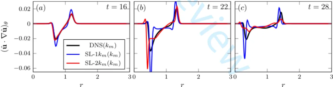
(a) t = 16 0 1 2 3 0.06 0.04 0.02 0 0.02 r (ˆu ·r ˆu )✓ DNS(km) SL-1km(km) SL-2km(km) (b) t = 22 0 1 2 3 r (c) t = 28 0 1 2 3 r
Figure 7. Mean Reynolds stresses in the azimuthal direction from DNS and semi-linear models at (a) t = 16, (b) t = 22 and (c) t = 28.
good agreement (figure 6a,c). Nevertheless, some deviations can be seen at t = 30, 40, in particular the first peak at small radius is not captured at t = 40. In addition, the maximum amplitude of the second harmonic reaches 1/3 of the maximum amplitude of the fundamental harmonic (figure 6c).
4.3. SL-2km semi-linear model
As seen in figures 3c and 6c, the second harmonic is triggered and reaches a non-negligible amplitude for both Re = 800 and Re = 2000. Its e↵ect can be taken into account by means of the semi-linear model (3.8-3.9), called SL-2km. Since the
For Peer Review
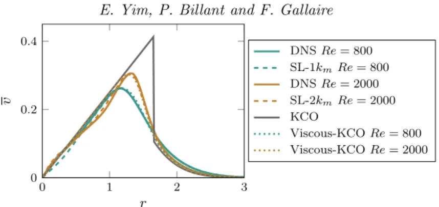
0 1 2 3 0 0.2 0.4 r v DNS Re = 800 SL-1kmRe = 800 DNS Re = 2000 SL-2kmRe = 2000 KCO Viscous-KCO Re = 800 Viscous-KCO Re = 2000Figure 8. Mean azimuthal velocity in the DNS and semi-linear models at t = 60 for Ro = 4 for Re = 800 and Re = 2000. KCO indicates the velocity distribution predicted by Kloosterziel et al. (2007) in the inviscid limit. Viscous-KCO corresponds to the velocity profile (5.11) which takes into account viscous e↵ects.
second harmonic is set to zero. Therefore, even if it is also unstable (figure 1b), its initial evolution is only due to the forcing by the fundamental harmonic.
For Re = 800 (figure 3c), the evolution of the amplitude of the first harmonic predicted by the SL-2km model (red continuous line) is slightly closer to the amplitude A(km) in
the DNS (black dashed line) than for the SL-1kmmodel (blue continuous line). However,
for Re = 2000 (figure 6c), the SL-2km(km) amplitude is not closer to A(km) in the DNS
than the SL-1kmmodel for 20. t . 30. The amplitudes of the second harmonic are also
well predicted by the SL-2km model. It reaches 15% and 26% of the amplitude of the
fundamental harmonic for Re = 800 and Re = 2000, respectively.
For Re = 2000, the predicted profiles for the mean azimuthal velocity for the SL-2km
model (figure 6b) are smoother than for the SL-1kmmodel (figure 6a). However, the first
peak near r⇠ 0.3 at t = 30 is less pronounced. To understand this discrepancy, we have plotted the Reynolds stresses in the ✓-direction in the DNS and the semi-linear models (figure 7). At t = 16, the SL-2kmmodel is in excellent agreement with the DNS, while at
t = 22 and t = 28, there are some departures especially at small radius (r⇡0.5). This is the reason why the SL-2kmmodel does not capture the first peak of the mean azimuthal
velocity (figure 6b).
Including higher harmonics might further improve the predictions. However, this would complicate the models while the primary goal of the present approach is the simplicity rather than the accuracy.
5. Final profiles of azimuthal velocity
The profiles of mean azimuthal velocity observed at late time t = 60, once the instability has ceased, have been compared to the theory of Kloosterziel et al. (2007) and Carnevale et al. (2011). As mentioned in the introduction, this theory states that the centrifugal instability homogenizes negative and positive absolute angular momentum L = r(v+r/Ro) so as to suppress negative gradients of L2under the constraint of absolute
angular momentum conservation. For anticyclones, the final profile of L in the inviscid limit is such that L is zero until a radius rcgiven byR
rc
0 rLidr = 0, where Li is the initial
absolute angular momentum. Beyond this radius, the velocity profile remains identical to the initial one. Therefore, the theoretical angular velocity is
⌦(r < rc) = 1
Ro, ⌦(r> rc) = exp( r
2). (5.1) Cambridge University Press
For Peer Review
Nonlinear evolution of the centrifugal instability using a semi-linear model 11 This profile (labelled KCO) is compared to those observed in the DNS and SL models for Re = 800 and Re = 2000 in figure 8. It is close to the observed profiles except in the vicinity of the radius rc where the latter are smooth while the theoretical profile is
discontinuous due to the inviscid approximation. In order to take into account viscous e↵ects, we have further considered the viscous di↵usion of (5.1). For large Reynolds number, the di↵usion equation
@⌦ @t = Re 1 @2⌦ @r2 + 3 r @⌦ @r . (5.2) shows that the angular velocity should decay slowly everywhere except in the vicinity of rc where radial derivatives are expected to be large because of the discontinuity.
To describe the local viscous evolution near rc, we therefore define a rescaled radial
coordinate ˜r =pRe(r rc) and we assume that ⌦ depends both on ˜r and the unscaled
radius r. We also introduce a slow time ⌧ = Re 1t. Hence, (5.2) becomes
@⌦ @t + 1 Re @⌦ @⌧ = @2⌦ @ ˜r2 + 1 p Re ✓ 2@ 2⌦ @ ˜r@r+ 3 r @⌦ @ ˜r ◆ + 1 Re ✓ @2⌦ @r2 + 3 r @⌦ @r ◆ . (5.3) Then, the solution is sought as an expansion in Reynolds number
⌦ = ⌦0+ Re 1/2⌦1+ Re 1⌦2+· · · . (5.4)
The zero-th and first order problems are @⌦0 @t = @2⌦ 0 @ ˜r2 , and @⌦1 @t @2⌦ 1 @ ˜r2 = 2 @2⌦ 0 @ ˜r@r + 3 r @⌦0 @ ˜r . (5.5) The solutions are chosen as
⌦0= A(r, ⌧ )erf ✓ r˜ 2pt ◆ + H(r, ⌧ ), and ⌦1= ✓ 2@A @r + 3 A r ◆ rt ⇡exp ✓ ˜r2 4t ◆ . (5.6) where A and H are arbitrary functions of r and ⌧ . These functions are found by considering the problem at order Re 1:
@⌦2 @t @2⌦ 2 @ ˜r2 = @⌦0 @⌧ + @2⌦ 0 @r2 + 3 r @⌦0 @r + 2 @2⌦ 1 @r@ ˜r + 3 r @⌦1 @ ˜r . (5.7) It can be shown that the solution ⌦2presents secular growth unless we set
@A @⌧ = @2A @r2 + 3 r @A @r, and @H @⌧ = @2H @r2 + 3 r @H @r. (5.8) The solutions are taken as
A =D exp ⇣ r2 B+4⌧ ⌘ (B + 4⌧ )2 + C, and H = E exp⇣ G+4⌧r2 ⌘ (G + 4⌧ )2 + F, (5.9)
where B, C, D, E, F and G are constants. We then impose that ⌦0at t = ⌧ = 0 matches
the profile (5.1). This implies B = G = 1, E = D = 1/2, F = C = 1/(2Ro). Then, the solution of (5.7) can be found
⌦2= p1 ⇡ ✓ @2A @r2 + 3 r @A @r + 3 4r2A ◆ ˜ rpt exp ✓ ˜ r2 4t ◆ . (5.10)
For Peer Review
Finally, the complete solution for ⌦ up to order Re 1, written back in terms of the
original variables r and t, reads ⌦ = Aerf p Re(r rc) 2pt ! + A 1 Ro+ 2@A @r + 3 rA ✓@2A @r2 + 3 r @A @r + 3 4r2A ◆ (r rc) r t ⇡Reexp ✓ Re(r r c)2 4t ◆ , (5.11) where A is given by (5.9) with the substitution r = r and ⌧ = Re 1t. The azimuthal
velocity profiles corresponding to (5.11) are plotted with dotted lines (viscous-KCO) in figure 8. The time in (5.11) has not been set to t = 60 but to t = 20. Indeed, since the profile (5.1) is the outcome of the centrifugal instability, we have assumed that it is virtually formed only at t = 40 once the instability has almost ceased. These viscous profiles are in much better agreement with the DNS than the inviscid profile of Kloosterziel et al. (2007) and Carnevale et al. (2011). Besides, we emphasize that the profiles in the DNS and SL models are in excellent agreement.
6. Conclusion
We have studied the nonlinear growth of the centrifugal instability in an anticyclone with Gaussian angular velocity in rotating fluids for Ro = 4. We have used an approach similar to the one behind the self-consistent model (Mantiˇc-Lugo et al. 2014). Using Reynolds decompositions (Reynolds & Hussain 1972) based upon a time average, Mantiˇc-Lugo et al. (2014) have separated the flow into mean flow and time harmonic fluctuations. These two components are coupled via Reynolds stresses in the mean flow equation and via the evolution of the mean flow in the fluctuation equation. In the present study on the centrifugal instability, we have used a spatial average instead of a time average and separated the flow into axially averaged mean flow and spatial harmonic fluctuation. Like for the self-consistent model, the fluctuation grows over an evolving mean flow while the mean flow is forced by the Reynolds stresses due to the fluctuations. They contribute to the progressive smoothing of the destabilizing vorticity, thereby reducing the instantaneous growth of disturbances. A similar saturating or stabilizing e↵ect is encountered in supercritical instabilities like vortex shedding behind a cylinder and flow over a cavity, although the Reynolds stresses can also be further destabilizing in subcritical flows like wall-bounded shear flows. The present semi-linear model with one harmonic is in very good agreement with DNS for Re = 800 and Re = 2000 concerning both the time evolution of the fluctuation amplitude and of the mean flow profiles. Including a second harmonic 2kminto the model improves slightly the predictions.
We have also compared the ‘final’ azimuthal velocity profile observed in the DNS and semi-linear models when the instability has disappeared to the inviscid profile proposed by Kloosterziel et al. (2007) based on homogenization of angular momentum towards a centrifugally stable flow. They agree except in the neighbourhood of the radius where the inviscid profile is discontinuous. To improve the prediction, we have computed asymptotically for large Reynolds number the viscous di↵usion of the theoretical profile of Kloosterziel et al. (2007). The discontinuity is then smoothed and the predicted profiles are in much better agreement with the profile observed in the DNS and semi-linear models.
The main interest of the present semi-linear models is their simplicity which may enable a deeper understanding of the underlying physics. In addition, we emphasize that they are very cheap in terms of computational cost. Indeed, the computing time for the present
For Peer Review
Nonlinear evolution of the centrifugal instability using a semi-linear model 13 3D DNS with the Nek5000 code takes 18 hours (elapsed real time) with 168 processors for 13 vertical wavelengths and for 100 time units. In contrast, a run of the semi-linear model with one or two harmonics only takes 6min or 10min, respectively with a single processor. This dramatic decrease on the computing time comes from the reduction of the problem to only few one-dimensional equations.
In the future, it would be interesting to investigate the connection between semi-linear models and amplitude equations derived from weakly nonlinear analyses. In addition, it would be interesting to develop similar models for non-axisymmetric centrifugal insta-bilities since they can be dominant in presence of background stratification (Lahaye & Zeitlin 2015; Yim et al. 2016, 2019). A similar approach could be also attempted for the two-dimensional shear instability by means of an azimuthal average.
Declaration of Interests. The authors report no conflict of interest.
REFERENCES
Batchelor, G. K. & Gill, A. E. 1962 Analysis of the stability of axisymmetric jets. J. Fluid Mech. 14 (4), 529–551.
Billant, P. & Gallaire, F. 2005 Generalized rayleigh criterion for non-axisymmetric centrifugal instabilities. J. Fluid Mech. 542, 365–379.
Carnevale, G. F., Kloosterziel, R. C., Orlandi, P. & Van Sommeren, D. D. J. A. 2011 Predicting the aftermath of vortex breakup in rotating flow. J. Fluid Mech. 669, 90–119. Carton, X., Flierl, G. R. & Polvani, L. M. 1989 The generation of tripoles from unstable
axisymmetric isolated vortex structures. EPL (Europhysics Letters) 9 (4), 339.
Deloncle, A., Billant, P. & Chomaz, J.-M. 2008 Nonlinear evolution of the zigzag instability in stratified fluids: a shortcut on the route to dissipation. J. Fluid Mech. 599, 229–239.
Fischer, P. F., Lottes, J. W. & Kerkemeier, S. G. 2008 Nek5000 Web page. http://nek5000.mcs.anl.gov.
Gent, P. R. & McWilliams, J. C. 1986 The instability of barotropic circular vortices. Geophys. Astrophys. Fluid Dyn. 35 (1-4), 209–233.
Hecht, F. 2012 New development in freefem++. J. Numer. Math. 20 (3-4), 251–265.
Ioannou, A., Stegner, A., Le Vu, B., Taupier-Letage, I. & Speich, S. 2017 Dynamical evolution of intense ierapetra eddies on a 22 year long period. J. Geophys. Res. 122 (11), 9276–9298.
Kloosterziel, R. C., Carnevale, G. F. & Orlandi, P. 2007 Inertial instability in rotating and stratified fluids: barotropic vortices. J. Fluid Mech. 583, 379–412.
Kloosterziel, R. C. & van Heijst, G. J. F. 1991 An experimental study of unstable barotropic vortices in a rotating fluid. J. Fluid Mech. 223, 1–24.
Lahaye, N. & Zeitlin, V. 2015 Centrifugal, barotropic and baroclinic instabilities of isolated ageostrophic anticyclones in the two-layer rotating shallow water model and their nonlinear saturation. J. Fluid Mech. 762, 5–34.
Lazar, A., Stegner, A. & Heifetz, E. 2013 Inertial instability of intense stratified anticyclones. part 1. generalized stability criterion. J. Fluid Mech. 732, 457–484. Mantiˇc-Lugo, V., C., Arratia, C. & Gallaire, F. 2014 Self-consistent mean flow description
of the nonlinear saturation of the vortex shedding in the cylinder wake. Phys. Rev. Lett. 113, 084501.
Mantiˇc-Lugo, V., C., Arratia, C. & Gallaire, F. 2015 A self-consistent model for the saturation dynamics of the vortex shedding around the mean flow in the unstable cylinder wake. Phys. Fluids 27 (7), 074103.
Meliga, P. 2017 Harmonics generation and the mechanics of saturation in flow over an open cavity: a second-order self-consistent description. J. Fluid Mech. 826, 503–521.
Rayleigh, Lord 1917 On the dynamics of revolving fluids. Proc. R. Soc. A 93 (648), 148–154. Reynolds, W. C. & Hussain, A. K. M. F. 1972 The mechanics of an organized wave in turbulent shear flow. part 3. theoretical models and comparisons with experiments. J. Fluid Mech. 54 (2), 263–288.
For Peer Review
Smyth, W. D. & McWilliams, J. C. 1998 Instability of an axisymmetric vortex in a stably stratified, rotating environment. Theor. Comp. Fluid Dyn. 11 (3-4), 305–322.
Synge, J. L. 1933 The stability of heterogeneous liquids. Trans. R. Soc. Canada 27, 1. Yim, E. & Billant, P. 2015 On the mechanism of the gent–mcwilliams instability of a columnar
vortex in stratified rotating fluids. J. Fluid Mech. 780, 5–44.
Yim, E., Billant, P. & M´enesguen, C. 2016 Stability of an isolated pancake vortex in continuously stratified-rotating fluids. J. Fluid Mech. 801, 508–553.
Yim, E., Stegner, A. & Billant, P. 2019 Stability criterion for the centrifugal instability of surface intensified anticyclones. J. Phys. Oceanogr. 49 (3), 827–849.