HAL Id: hal-03083636
https://hal.archives-ouvertes.fr/hal-03083636
Submitted on 8 Jan 2021
HAL is a multi-disciplinary open access
archive for the deposit and dissemination of
sci-entific research documents, whether they are
pub-lished or not. The documents may come from
teaching and research institutions in France or
abroad, or from public or private research centers.
L’archive ouverte pluridisciplinaire HAL, est
destinée au dépôt et à la diffusion de documents
scientifiques de niveau recherche, publiés ou non,
émanant des établissements d’enseignement et de
recherche français ou étrangers, des laboratoires
publics ou privés.
of Fault Slip and Geothermal Subsidence
John Dale B. Dianala, Romain Jolivet, Marion Y. Thomas, Yo Fukushima,
Barry Parsons, Richard Walker
To cite this version:
John Dale B. Dianala, Romain Jolivet, Marion Y. Thomas, Yo Fukushima, Barry Parsons, et al.. The
Relationship Between Seismic and Aseismic Slip on the Philippine Fault on Leyte Island: Bayesian
Modeling of Fault Slip and Geothermal Subsidence. Journal of Geophysical Research : Solid Earth,
American Geophysical Union, 2020, 125 (12), pp.e2020JB020052. �10.1029/2020JB020052�.
�hal-03083636�
Bayesian Modeling of Fault Slip
and Geothermal Subsidence
John Dale B. Dianala1,2 , Romain Jolivet3,4 , Marion Y. Thomas5 , Yo Fukushima6 ,
Barry Parsons1, and Richard Walker1
1COMET, Department of Earth Sciences, University of Oxford, Oxford, UK,2National Institute of Geological
Sciences, University of the Philippines Diliman, Quezon City, Philippines,3Laboratoire de Géologie, Département de
Géosciences, École Normale Supérieure, PSL Université, UMR 8538, Paris, France,4Institut Universitaire de France, Paris, France,5Sorbonne Université, CNRS-INSU, Institut des Sciences de la Terre Paris, ISTeP UMR
7193, Paris, France,6International Research Institute of Disaster Science, Tohoku University, Sendai, Japan
Abstract
Delineating seismic and aseismic slip on faults allows the exploration of the complex relationship between these different modes of slip. Further, quantifying them helps in the assessment of seismogenic potential. We present a distributed slip model of the rate of aseismic slip along the Leyte island section of the Philippine Fault and make comparisons with the extent of seismic slip from the latest significant earthquakes in July 2017. We derived both coseismic and aseismic slip distributions from kinematic inversions of synthetic aperture radar interferometric (InSAR) observations using a probabilistic (Bayesian) framework. Velocity maps from stacking and time series analysis of ALOS interferograms spanning 4 years (2007–2011) show a step change in ground deformation right on the fault. Inverting for slip at depth reveals along-strike variations of aseismic slip rate over ∼100 km. Aseismic slip on the surface reaches rates of more than 3 cm/yr, equivalent to the long-term slip rate (3.3 ± 0.2 cm/yr). Over the same period, a 20-km segment in Tongonan appears to be locked. This segment ruptured in Mw6.5 and Mw5.8 earthquakes on 6 and 10 July 2017, respectively, as constrained by Sentinel-1 and ALOS-2 InSAR data. Seismic slip appears to be restricted within the Tongonan segment, with up to 152 ± 21 cm of left-lateral displacement. The slip budget and complementarity between the extents of interseismic and coseismic slip suggest that a seismogenic asperity exists in Tongonan. The presence of active hydrothermal systems and rate-strengthening materials provide physical conditions that can promote aseismic slip.Plain Language Summary
In July 2017, the Philippine Fault on Leyte island produced a damaging earthquake that was unexpected. Previous studies that tracked the movement of the Earth's crust have suggested that the fault in Leyte does not accumulate strain, and hence stress, as the fault primarily slides stably and slowly. This is in contrast to earthquake-generating faults that go on a cycle of building up stress for a long period of time, due to the crust staying stuck (or locked) on the fault, and then releasing the stored stress as an earthquake. With analysis of high-resolution satellite radar, we now show that while 100 km of the fault indeed appears to be moving slowly and gradually, a 20-km-long portion in the middle of the fault appears to be locked. Our observations and models of the July 2017 earthquake confirm that this same section of the fault alone moved then. The geometry of the fault, the abundance of fluids, and the presence of specific types of minerals may all play a role on how the fault behaves. This work is the first of its kind on the Philippine Fault, highlighting the importance of exploring relatively less well studied faults and their physical properties.1. Introduction
Faults that slip aseismically, as opposed to locked faults, are often considered less likely to generate large earthquakes due to the lack of long-term strain accumulation. Hence, the seismogenic potential of faults can be assessed by appraising the degree and extent of locking on faults and by exploring the relationship between seismic and aseismic slip (Avouac, 2015; Harris, 2017). Geodetic and seismological observations
Key Points:
• We present the first probabilistic model of interseismic aseismic slip throughout seismogenic depth along 100 km of the Philippine Fault
• Joint inversion for anthropogenic subsidence and fault deformation reveals downdip locking from the surface on a 20-km section in Tongonan
• Extent of seismic rupture of the July 2017 magnitude 6.5 and 5.8 earthquakes correlates with geometric complexity and lack of slip deficit Supporting Information: • Supporting Information S1 Correspondence to: J. D. B. Dianala, john.dianala@earth.ox.ac.uk; jddianala@nigs.upd.edu.ph Citation: Dianala, J. D. B., Jolivet, R., Thomas, M. Y., Fukushima, Y., Parsons, B., & Walker, R. (2020). The relationship between seismic and aseismic slip on the Philippine Fault on Leyte Island: Bayesian modeling of fault slip and geothermal subsidence.
Journal of Geophysical Research: Solid Earth, 125, e2020JB020052. https:// doi.org/10.1029/2020JB020052
Received 23 APR 2020 Accepted 20 OCT 2020
Accepted article online 24 OCT 2020
©2020. The Authors.
This is an open access article under the terms of the Creative Commons Attribution License, which permits use, distribution and reproduction in any medium, provided the original work is properly cited.
show that fault segments that appear to slip aseismically on the surface may host locked sections at depth. This has been made apparent on relatively well studied faults in California (USA) (e.g., Burgmann et al., 2000; Chaussard et al., 2015; Jolivet, Simons, et al., 2015; Johnson, 2013; Lienkaemper et al., 2012; Tse et al., 1985), most strikingly along the central section of the San Andreas Fault, where the Parkfield segment has hosted repeated strong earthquakes on a locked asperity (e.g., Bakun et al., 2005). Continen-tal faults in other settings, including the Longitudinal Valley Fault (Taiwan) and the Alto Tiberina Fault (Italy), also show a similar behavior of partial locking with a potential for strong earthquakes (e.g., Anderlini et al., 2016, and Thomas, Avouac, Champenois, et al., 2014, respectively). In addition, numerical models based on rate-and-state friction suggest that seismic ruptures may propagate across sections of faults that host aseismic slip during the interseismic period (e.g., Noda & Lapusta, 2013; Thomas et al., 2017). Isolating seismogenic asperities and documenting how far seismic slip propagates into sections that slip aseismically is therefore key in estimating seismic hazard, especially when these faults run across populated regions. Many advances in understanding the diverse spatial and temporal nature of aseismic slip on continen-tal faults have been brought about by interferometric synthetic aperture radar (InSAR) (Bürgmann, 2018; Jolivet & Frank, 2020). Thanks to its fine resolution, global coverage, and convenient access to the data, space geodesy using InSAR has become a powerful tool for studying earthquakes and active tectonics (Elliott et al., 2016). The earliest InSAR observations of the seismic cycle revolutionized our ability to explore fault and crustal mechanics (e.g., Deng, 1998; Massonnet et al., 1993; Peltzer et al., 2001; Price & Sandwell, 1998; Wright et al., 2001). Continuous monitoring through interseismic periods has further enabled us to delin-eate aseismic slip on remote and less well instrumented faults (e.g., Cavalié et al., 2008; Cetin et al., 2014; Jolivet et al., 2013; Fattahi & Amelung, 2016; Pousse Beltran et al., 2016; Thomas, Avouac, Champenois, et al., 2014; Tong et al., 2018). This allows us to discover and explore potential earthquake sources that might not be well known, like on faults sometimes referred to as “creeping faults” (e.g., Jolivet, Simons, et al., 2015). For two decades, shallow aseismic slip of more than 2.0 cm/yr on the Leyte island section of the Philippine Fault has been measured using sparse GPS surveys alone (Duquesnoy et al., 1994; Duquesnoy, 1997) (Figure 1). The similarity of these estimates to the long-term slip rate, along with the lack of induced seis-micity from injection experiments, has led to the notion that this portion of the fault is primarily aseismic (Prioul et al., 2000). However, on 6 July 2017, a moment magnitude (Mw) 6.5 earthquake occurred in Leyte
(Fukushima et al., 2019; PHIVOLCS, 2017; Yang et al., 2018). With up to 1.1 m of slip on the surface, most prominently in the village of Tongonan, within the city of Ormoc, the Mw6.5 earthquake registered Inten-sity VIII shaking (on the PHIVOLCS Earthquake IntenInten-sity Scale) near the epicenter (Llamas et al., 2017; PHIVOLCS, 2017). The temblor happened in populated areas, resulting to three deaths and widespread economic disruption (PHIVOLCS, 2017). InSAR has been used to model the extent of seismic slip (Yang et al., 2018) and to juxtapose the seismogenic section with the surface manifestation of aseismic slip in the interseismic (Fukushima et al., 2019). However, anthropogenic subsidence adjacent to the fault and the coe-seismic area has hindered detailed comparisons of intercoe-seismic and cocoe-seismic slip distribution (Fukushima et al., 2019). Furthermore, abundant geothermal resources in Leyte have spurred more than 30 years of detailed geological investigations on and near the fault, even up to around 2 km depth (e.g., Caranto & Jara, 2015; Reyes, 1990; Scott, 2001), allowing the rare opportunity to directly correlate in-situ physical conditions of an active fault with its behavior.
In this study, we constrain interseismic deformation from fault and anthropogenic subsidence sources in Leyte and analyze the relationship between aseismic and seismic slip modes. The distributed slip models that we present are the first of their kind on the Philippine Fault, as we invert for the subsidence parameters and slip rates through probabilistic (Bayesian) approaches. This permits us to explore how fault zone geometry and geological conditions correlate and might control the distribution of the slip modes, adding to a rich body of literature on fault and earthquake mechanics. Independent of the available InSAR data, we incorporate information from leveling surveys (from Apuada et al., 2005) to understand the anthropogenic subsidence source. For coseismic displacements, we isolate the slip of the July 2017 mainshock from that of a Mw5.8
aftershock, which are combined in previous coseismic slip models (Fukushima et al., 2019; Yang et al., 2018), and this shows how the spatiotemporal distribution of seismic slip might relate to geometrical complexity of the fault. Finally, we provide a physics-based framework for estimating the earthquake return time in a probabilistic sense and check this against the possibility of the July 2017 earthquake as a repeat of a surface magnitude (Ms) 6.9 event in 1947 (Fukushima et al., 2019), which is of societal importance.
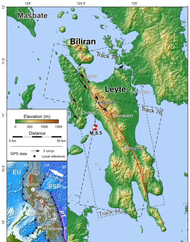
Figure 1. Active tectonics of the island of Leyte in the Philippines. Shaded relief map is based on SRTM 30-m resolution elevation data. Surface trace of the
Philippine Fault (red, modified from Tsutsumi & Perez, 2013) is based on observations from AirSAR-derived DEM and InSAR. Arrows are GPS-derived
velocities from Duquesnoy (1997) relative to a local reference station (black diamond). Red “beach ball” indicates the mechanism of the 6 July 2017 Mw6.5
earthquake (USGS). Long and short black dashed lines indicate spatial coverage of ALOS data in ascending (Track 443) and descending (Tracks 76 and 77) passes, respectively. Inset: Geographic location of Leyte (white box) with respect to regional tectonic features around the Philippine Mobile Belt (shaded area)
(modified from Aurelio et al., 2013). White circles=epicenters of known historical and recent surface-rupturing earthquakes (see text for discussion):
L=Luzon, magnitude Mw7.7, 1990; R=Ragay Gulf, Ms7.3, 1973; M=Masbate, Ms6.2, 2003; S=Surigao, Ms6.9,1879 and Mw6.5, 2017. White arrow
indicates the velocity of the Philippine Sea Plate (PSP) relative to the Eurasian Plate (EU) (DeMets et al., 2010). Sawtooth pattern: subduction zones, with PT denoting the Philippine Trench.
2. Tectonic Setting
2.1. The Philippine Fault: Geodynamic and Seismic Context
The Philippine Fault is an approximately 1,200-km-long left-lateral strike-slip fault (Allen, 1962; Tsutsumi & Perez, 2013). It accommodates part of the the oblique convergence between the Philippine Sea Plate and the Philippine Mobile Belt, on the margin of the Eurasian Plate, in a strain partitioning regime (Aurelio, 2000; Barrier et al., 1991) (Figure 1). The Philippine Sea Plate moves northwestward at around 8.8 cm/yr rel-ative to a fixed Eurasian Plate (DeMets et al., 2010). Regional Euler pole rotation suggests that the Philippine Fault has a long-term strike-slip rate of 1.9–2.5 cm/yr (Barrier et al., 1991). In the northern Philippines, 100–150 km-long GPS transects indicate a long-term slip rate of 2.4–4.0 cm/yr on the Philippine Fault (Galgana et al., 2007; Yu et al., 2013). These estimates, however, go across several branches of the fault on Luzon island. More detailed block models from campaign surveys suggest interseismic slip rates of around 0.7 to 3.1 cm/yr on individual branches of the Philippine Fault in Luzon (Hsu et al., 2016).
Geologic, geodetic, and seismotectonic studies have shown a spectrum of fault slip behavior along differ-ent sections of the Philippine Fault. The location of several major modern and historical earthquakes are associated with northern and southern splays of the Philippine Fault (Bautista & Oike, 2000). However, only a handful have been determined to have produced surface ruptures, like the 1990 magnitude Mw7.7
Luzon (Punongbayan et al., 1992; Silcock & Beavan, 2001), the 1973 Ms7.3 Ragay Gulf (southern Luzon)
(Tsutsumi et al., 2015), and the 1879 Ms6.9 and 2017 Mw6.5 Surigao (Mindanao) (Perez & Tsutsumi, 2017;
PHIVOLCS, 2018) earthquakes. The central section of the fault (from 10–12.5◦N) is known for clusters of moderate to strong earthquakes (∼M 5–6), including the surface-rupturing 2003 Ms6.2 Masbate earthquake (Bacolcol et al., 2005). It has also been suggested that the Masbate earthquake was followed by postseismic afterslip (Besana & Ando, 2005). In addition, directly south of Masbate, aseismic slip on the island of Leyte was first quantified from campaign GPS surveys around the Tongonan geothermal area in northern Leyte. Fault-parallel aseismic slip rates on the surface range from 2.6 cm/yr (Duquesnoy et al., 1994) to 3.5 cm/yr (Duquesnoy, 1997; Prioul et al., 2000). As previously mentioned, the 6 July 2017 Mw6.5 earthquake ruptured
the section of the fault where these surveys were conducted. 2.2. Seismotectonics of Leyte Island
The Philippine Fault goes through the island of Leyte from its northern to its southern shores, with a marked 150-km-long onshore trace. At the latitude of the island, the fault crosses the volcanic arc associated with the Philippine Trench subduction zone (Barrier et al., 1991) (inset of Figure 1). The fault is especially clear on narrow linear valleys and portions that cut through Quaternary volcanoes and the central highlands (Allen, 1962; Aurelio et al., 1993; Lagmay et al., 2003; Tsutsumi & Perez, 2013; Willis, 1944).
Active fault maps, based on topographic data from aerial photos and 90-m resolution global digital elevation models (PHIVOLCS, 2016; Tsutsumi & Perez, 2013), reflect the main fault trace as a linear feature along the length of the island, with a bend near Tongonan village. There, subparallel secondary faults east of the main trace demarcate a 2- to 2.5-km-wide relay zone that, further south (west of Burauen in Figure 2a), becomes a 4-km-wide left-stepping step-over at around 11◦N. Structural field observations and tectonic models expound on localized extension and secondary faulting along this releasing bend (Aurelio et al., 1993; Duquesnoy et al., 1994) and the sigmoidal structures that result from long-term volcano-tectonic interactions (Lagmay et al., 2003). The Leyte Geothermal Production Field in Tongonan has been exploiting the abundant geothermal resources related to the Quaternary volcanoes for commercial energy production since the 1980s. Geothermal exploitation within the fault bend leads to subsidence of up to 3 cm/yr (Apuada et al., 2005). South of Tongonan, a rift-like morphology can be observed on the wide valleys west of Burauen, which Willis (1944) attributes to be a part of a “Visayan Rift.” Subsequent mapping by Allen (1962) describes the active left-lateral strike-slip kinematics. The most recent work by Tsutsumi and Perez (2013) does not map out structures west of the main trace as active.
Several studies focusing on geothermal energy exploration suggest that the faulting (e.g., Aurelio et al., 1993; Lagmay et al., 2003) and continuous aseismic slip (Caranto & Jara, 2015) on the Philippine Fault in the volcanic area enhances the permeability in the shallow crust, allowing for the outflow of geothermal fluids. Duquesnoy et al. (1994) propose that the high heat flow and the clay alteration of volcanic rocks, due to the hydrothermal activity, might affect the rheology of the fault zone. They postulate that this causes the weakening of the fault zone, which, in turn, promotes aseismic slip.
(a)
(b)
Figure 2. Seismotectonics of Leyte island. (a) Main Philippine Fault segments referred to in the text (red line), along with secondary structures (dashed black
lines) and surface exposures of ophiolitic rocks (Aurelio et al., 1993; Guotana et al., 2018; Suerte et al., 2005). (b) Instrumental seismicity (1984 to July 2017) in Leyte based on the rebuilt International Seismological Centre (ISC) catalog (Storchak et al., 2017). Symbol sizes are scaled according to surface wave magnitude
(Ms). The mechanism and location of the July 2017 mainshock reported by the USGS is shown for reference (red beach ball).
The ophiolitic basement is also exposed on the surface in Leyte (Aurelio et al., 1993; Cole et al., 1989; Dimalanta et al., 2006; Guotana et al., 2018; Suerte et al., 2005), as shown in Figure 2. While the mineralogy of serpentinites from ophiolites along the San Andreas Fault has been considered to explain aseismic slip (e.g., Moore & Rymer, 2007), this has yet to be suggested for the Philippine Fault, so we expound on this in detail in the discussion (section 5).
Fukushima et al. (2019) show the along-strike variability of surface aseismic slip rates based on the step change of InSAR-derived surface velocity. However, due to the large magnitude of subsidence in the geother-mal area, they are unable to estimate the rate of interseismic aseismic slip where the 2017 earthquake happened.
We focus this paper on two main segments of the Philippine Fault in Leyte, which are primarily based on distinct continuous surface traces: the Northern Leyte Segment (the section of the fault from Leyte town to Ormoc) and the Central Leyte Segment (from Burauen to Abuyog) (Figure 2a). Plotting the reviewed catalog of the International Seismological Centre (ISC; Storchak et al., 2017) of seismic events from 1964 to just before the July 2017 earthquake shows a clustering of seismicity in northern Leyte, which con-trasts with what can be seen in central Leyte (Figure 2b). Besana and Ando (2005) have implied that a “large” earthquake in 1608 ruptured the Central Leyte Segment and may suggest that a “seismic gap” exists between Burauen and Abuyog. Bautista and Oike's (2000) review of the preinstrumental historical record of
Table 1
Summary of ALOS SAR Data per Track Used for Interseismic Time Series Analysis and Stacking
Date range Track # of acquisitions # of interferograms Nvalida
2006/12 to 2011/01 443, Ascending 25 86 50
2006/10 to 2011/01 76, Descending 5 10 6
2008/09 to 2010/12 77, Descending 3 3 2
Note. Dates are formatted as yyyy/mm.
aNumber of required coherent measurements from interferogram network on a pixel to make a velocity
estimate.
earthquakes in the Philippines, however, suggests that the 1608 earthquake had a Msof 5.0 and a poorly
con-strained location (i.e., this event only has two reports that could be used as basis for the equivalent Modified Mercalli intensity). In southern Leyte, seismicity broadly clusters to the east of the fault trace.
3. Interseismic (2007–2011) Velocity Field and Aseismic Fault Slip
In this section, we explore the aseismic slip throughout the fault in Leyte including where the anthropogenic subsidence occurs. By deriving high-resolution velocity maps from InSAR data and including a subsidence source in the kinematic inversions, we are able to isolate the strike-slip fault deformation. We generated line-of-sight velocity maps with a spatial resolution of around 100 m in radar range (nominally of higher resolution compared to the 1,500-m resolution velocity maps in Fukushima et al., 2019). This allows us not only to to revisit the surface manifestation of shallow aseismic slip on the fault but also to capture the anthropogenic subsidence in enough detail that corresponds to data from local leveling surveys (Apuada et al., 2005).
3.1. InSAR Data Processing
Using available synthetic aperture radar (SAR) data from ascending and descending passes of the ALOS satellite (Table 1), we analyze the surface deformation on Leyte during the 2007 to 2011 interseismic period. Because there has not been any large earthquake in the area in the 70 yr prior to the 2017 earthquake, we do not expect significant postseismic transient motion, and we can be confident that the ALOS measurements capture only interseismic motion. ALOS L-band SAR data (wavelength,𝜆 = 23.6 cm) has the advantage of being able to produce coherent interferograms in vegetated areas despite long temporal baselines (e.g., Pousse Beltran et al., 2016; Sandwell et al., 2008), unlike SAR data at shorter wavelengths (e.g., C and X bands).
We used the GAMMA Software to produce unwrapped interferograms from single-look complex images (SLC). For each track, we coregistered all SLCs to a corresponding reference SLC. Reference SLCs for Tracks 443, 76, and 77 were chosen as a compromise between the perpendicular baseline of individual interfero-grams and overall baseline extent of the whole interferogram network. We first generated interferointerfero-grams and multilooked them to a pixel size of around 100 m × 100 m in azimuth and range. We used an adap-tive spectral filter to improve the signal-to-noise ratio while preserving high-phase gradients (Goldstein & Werner, 1998). We unwrapped the interferograms using a minimum cost flow (MCF) algorithm (Werner et al., 2002) and masked decorrelated pixels (i.e., those with coherence less than 0.4). We manually corrected unwrapping errors between adjacent islands with less than 2𝜋 phase jumps and no expected relative motion (i.e., islands that are on the same side of the fault). For removal of the topographic phase and generating a lookup table for geocoding the data, we used an airborne SAR-derived “bare-Earth” digital elevation model (DEM) from the National Mapping and Resource Information Authority of the Philippines (NAMRIA) (e.g., Luzon et al., 2016). For computational efficiency, we downsampled the 5-m resolution NAMRIA DEM to 10-m resolution.
3.1.1. Estimating Surface Deformation Rates
As the temporal coverage of the ascending and descending passes are not uniform (see supporting information Figures S1–S3 for temporal and spatial baselines, and interferogram pairs), we employed dif-ferent strategies to measure the surface deformation rate. The ascending track has 25 acquisitions between December 2006 and February 2011 and covers the whole length of the fault in Leyte. The two descending tracks that cover the fault have fewer acquisitions. Data from Track 76 encompasses most of central and
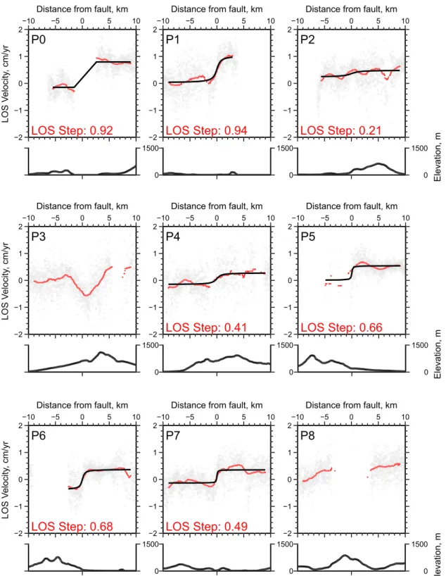
Figure 3. Interseismic surface deformation in Leyte in satellite line-of-sight (LOS) with rates in cm/yr (positive values indicate movement toward the satellite),
and the Philippine Fault as the solid black line. Gray areas within the velocity field correspond to pixels masked out due to temporal decorrelation. (a) Surface
deformation from time series analysis of ascending ALOS data (Track 443). The 6 July 2017 mainshock (Mw6.5) location is shown for reference. LOS velocity
swath profiles, P0–P8, are in Figure 4. (b) LOS displacement rate derived from stack of ALOS descending interferograms (Tracks 76 and 77).
southern Leyte and has five acquisitions from 2006 to 2011. Track 77, which covers northern Leyte and Biliran, has only three acquisitions between 2008 and 2011.
For the ascending track, we followed an N-SBAS (Small Baseline) time series analysis approach imple-mented in the Generic InSAR Analysis Toolbox (GIAnT; Agram et al., 2013). This method allows the estimation of velocities in areas that have decorrelated signals in some interferograms but have at least a specific number of coherent measurements (N) in the interferogram network (e.g., Doin et al., 2011; Jolivet et al., 2012). For the time series inversion, we manually selected 86 interferograms with no apparent nonlinear phase ramps, which are usually due to ionospheric perturbations (Gomba et al., 2016). The result-ing interferogram network still covers 4 yr of data (from 2007–2011, as shown in supportresult-ing information Figure S1). We estimated the LOS velocity for pixels where more than 50 interferograms are unwrapped, assuming a linear rate. We included a step function in time to remove the coseismic signal from a Mw5.3
earthquake in southern Leyte that has visible surface deformation off the Philippine Fault. Prior to inverting for the LOS velocity, we applied atmospheric corrections based on the European Centre for Medium-Range Weather Forecasting ERA-Interim models (Jolivet et al., 2014). We also removed planar ramps on individ-ual interferograms and corrected for DEM errors. The resulting velocity map has a mean root-mean-square error of 1.3 cm/yr (supporting information Figure S4a).
For the descending tracks, we did not perform a complete time series analysis to derive deformation rates as we do not have enough acquisitions. Instead, we estimated the average LOS displacement rate, ̇𝜙d, through a simple yet robust stacking approach, implemented in GAMMA, from the unwrapped interferograms. For N number of interferograms, the algorithm uses the temporal baseline, Δtj, of the respective j interferograms
as a weight for LOS displacement,𝜙j, to derive ̇𝜙d, as
̇𝜙d= ∑N 𝑗=1Δt𝑗𝜙𝑗 ∑N 𝑗=1Δt2𝑗 . (1)
Similar to the N-SBAS time series approach, this formulation lets us estimate deformation rate on pixels that have coherent signals in N number of interferograms in the stack. We set N to to be more than half the total number of interferograms of each stack (Table 1). The mean standard deviation for the descending Tracks 76 and 77 stacks are around 1.1 and 0.9 cm/yr, respectively (supporting information Figure S4b).
3.1.2. Deriving Subsidence From InSAR
The LOS velocity maps show a sharp velocity gradient across the Philippine Fault (Figure 3). We measure 0.2 to 0.9 cm/yr difference in the ascending LOS velocity across the fault with a step-like function right on the fault (Figure 4). Motion is compatible with the left-lateral sense of slip on the fault, as shown by the opposite LOS deformation rate observed on ascending versus descending tracks. We also observe an elliptical deformation feature that is most likely related to subsidence adjacent to the fault. Leveling surveys by Apuada et al. (2005) indicate up to 18 cm of subsidence in the Leyte Geothermal Production Field between 1997 and 2003. They associate this phenomena with net mass loss from energy production, as extraction rates exceed fluid reinjection rates. Since the geothermal production is ongoing, it is likely that subsidence still occurs in the area.
With InSAR displacements from multiple LOS directions, we can derive horizontal and vertical velocity components and provide new measurements of subsidence. The off-nadir LOS of the SAR satellites makes InSAR most sensitive to vertical deformation; nonetheless, it is also possible to derive the eastward and northward component of horizontal motion (e.g., Fialko et al., 2001; Wright et al., 2004). As we lack a third velocity vector, however, we are unable to independently constrain the eastward and northward components of horizontal motion. We can instead project the east and north horizontal components of the InSAR LOS to the dominant horizontal direction of movement around the fault (as in Lindsey et al., 2014; Tymofyeyeva & Fialko, 2018).
Given the LOS velocity from ascending ( ̇𝜙a) and descending ( ̇𝜙d) tracks, we inverted for vertical and fault-parallel velocity components, Vvand Vf, respectively, as
[ ̇𝜙a ̇𝜙d ] = [ easin(𝛼) + nacos(𝛼) ua edsin(𝛼) + ndcos(𝛼) ud ] [ V𝑓 Vv ] , (2)
where e, n, and u are the east, north, and up components, respectively, of the unit vector pointing toward the satellite.𝛼 is the average strike of the Philippine Fault (328◦), which corresponds to its large-scale strike-slip nature, and is, to first order, consistent with the GPS observations (Duquesnoy, 1997) (Figure 1).
To maintain temporal consistency, we derived the ascending LOS displacement rate for this inversion from stacking interferograms (as in section 3.1.1) that cover the same time period as the descending track (2008–2010). The derived fault-parallel and vertical velocities are shown in Figure 5.
3.2. Manifestation of Surface Aseismic Slip
The LOS velocity map from the ALOS ascending track data shows a clear discontinuity across the fault (Figures 3a and 4, Profiles P0, P1, and P4 to P7). This is apparent on a ∼100-km-long section of the fault, albeit discontinuously, between 10.5◦N and 11.5◦N. Comparing the LOS velocity with the elevation on the same profiles suggests that this step change does not correlate to elevation gradients. The contrast in sur-face velocity, however, coincides with well-preserved fault scarps and most of the mapped sursur-face trace of the Philippine Fault (as in Tsutsumi & Perez, 2013) in the northern and central sections of the island. We therefore attribute the velocity step to aseismic slip on the surface. Surface deformation derived from the
Figure 4. ALOS ascending track (443) LOS velocities and step change (in cm/yr) within 20-km-long, 1-km-wide swath profiles centered on the Philippine Fault
in Leyte (see Figure 3 for location). Corresponding elevations are shown below each profile. Gray dots and red line represent the LOS velocity and median value, respectively. Black lines indicate the step function fit to the median LOS velocity (see Appendix A).
(a)
(c)
(b)
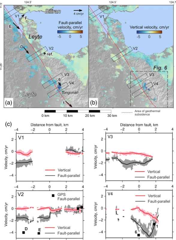
Figure 5. Estimated fault-parallel and vertical velocity in northern Leyte. (a) Fault-parallel velocity from InSAR
analysis. Black boxes show the spatial extent of swath Profiles V1 to V4. Black vectors are GPS velocities from Duquesnoy (1997) (same as Figure 1) relative to the reference station (black diamond), with station names outlined in white. (b) Same, but showing the vertical velocity and the geothermal subsidence area (based on Apuada et al., 2005) in Tongonan (dotted outline). (c) Profiles of fault-parallel velocity (gray: data, black: median) and vertical velocity (pink: data, red: median) from Swaths V1–V4. V2 shows a clear step function in fault-parallel velocity right on the fault, which is absent in V3. This suggests that shallow aseismic slip on the fault occurs near the surface at V2, but not on V3. The fault-parallel component of Duquesnoy (1997) GPS data (black squares) are shown in provile V2 for reference.
descending track acquisitions (Figure 3b) has a lot more spatial variability and observation gaps. This is likely due to consistent temporal decorrelation of interferograms, resulting to less than the N number of obser-vations required to estimate the average velocity. We nevertheless still observe a contrast in the descending LOS velocity across the fault, as also noted by Fukushima et al. (2019). We describe below in more detail the deformation field, from north to south.
North of 11.4◦N, while the Philippine Fault disappears below water in the strait between Leyte and Biliran, we observe a clear difference in velocity between the two islands, which are on opposite sides of the fault (P0 in Figures 3 and 4). Although unwrapping across water requires the assumption that no significant phase jump exists between landmasses, we are confident that the consistency between surface deformation rates in Leyte and Biliran suggests our velocity field is robust. In the town of Leyte, just north of Profile P1, field observations and anecdotal reports suggest that roads, houses, and other concrete structures show signs of left-lateral displacement even if there are no significant seismic events (supporting information Figures S5b and S5c). Profiles V1 and V2, in Figure 5, highlight the fault-parallel motion across the fault between the islands of Leyte and Biliran and onshore in northern Leyte, respectively. They both correspond to left-lateral motion, which on Profile V2 is a clear step function of 2 cm/yr right on the fault. This signifies that, for this time period at least, the northern section of the fault in Leyte slipped aseismically at around the long-term rate near the surface. The GPS fault-parallel velocities from Duquesnoy (1997) (black squares in Profile V2) appear to suggest faster motion than the InSAR data across the fault. This may reflect temporal variations on the interseismic slip rate in this location, but the sparse GPS data coverage makes it difficult to make robust inferences.
Contrast in surface velocities across the Philippine Fault is less prominent on Profile P2 (Figure 4), north of Tongonan. The derived fault-parallel surface velocity also shows no discontinuity across the fault in this area (Figure 5c, Profile V3), possibily indicating that the fault is locked near the surface. Another possibility is that the aseismic slip signal between Profiles P2 and P3, if any, might be obscured by the subsidence-related deformation in Tongonan (Profile V4 in Figure 5c). Finally, significant surface ruptures related to the 6 July 2017 Mw6.5 earthquake are found just south of Profile V4 (PHIVOLCS, 2017).
Along the central highlands in Leyte, temporal decorrelation leads to gaps in the LOS velocity maps near the fault. Still, LOS velocity steps are visible across the fault from Burauen down to Abuyog, between 11◦N and 10.6◦N (Profiles P4 to P7 in Figure 3). In the field, continuous and slow offset of roads in Abuyog have been documented by Tsutsumi et al. (2016). One of these roads has been repaved recently, but it appears the prerepavement displacement has been preserved (supporting information Figure S5d).
South of Abuyog, no clear contrast in the LOS velocity is observable (e.g., P8 in Figure 3). However, it does not necessarily mean that the fault does not slip aseismically near the surface. The ascending track LOS is orthogonal to the fault in this area, which makes fault-parallel deformation, if it exists, unresolvable. Looking at the descending data, which has a LOS oblique to the fault, there does appear to be a difference in the far-field velocities across the fault. However, we lack sufficient coherent data to be able to resolve the deformation rates closer to the fault. The off-main trace faulting in southern Leyte (Figure 2a) might also mean that deformation is more distributed across a wider area.
3.3. Subsidence in Tongonan
Our analysis of LOS surface velocities makes it apparent that to delineate the expression of shallow aseismic slip, we need to understand the contribution of the subsidence source to the deformation field adjacent to the fault. The vertical displacement rate, as seen in Figure 5b, shows subsidence in an area previously monitored by leveling surveys (Apuada et al., 2005). We estimate up to ∼2.5 cm/yr of subsidence (Profile V4, Figure 5c), which is slightly less than the reported ∼3 cm/yr of maximum subsidence from the geothermal survey by Apuada et al. (2005). This discrepancy may be due to temporal variations in net mass loss, especially as a gradual decrease in extraction rates since the early 2000s has been reported (Hazel et al., 2015). We also note a significant amount of horizontal motion in the subsidence area (Profile V4 in Figure 5c), but in the opposite direction of that corresponding to left-lateral slip on the fault (see Profiles V1 and V2, Figure 5c). Since both ascending and descending tracks are not consistently coherent in this area, we cannot derive meaningful horizontal and vertical deformation rate maps there. However, the apparent horizontal motion in Profile V4 may be related to the subsidence, in which case, it represents the surface moving toward the area of peak subsidence.
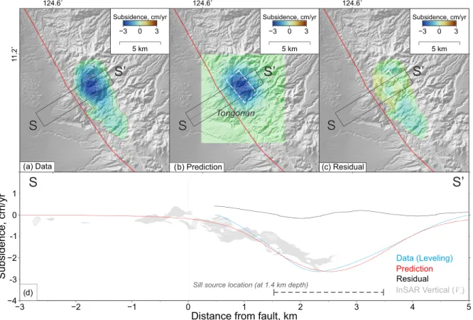
Figure 6. Subsidence data, model prediction, and residuals from modeling using leveling data (Apuada et al., 2005). (a) Interpolated subsidence rates based on
leveling contours, with extent of swath profile, S-S′(black rectangle). The outermost contour represents zero subsidence as published in Apuada et al. (2005),
and each contour interval represents 0.2 cm/yr of subsidence. (b) Predicted subsidence from the optimal source model geometry, with the surface projection of the sill source (white dashed polygon). (c) Residual deformation (the difference between data and predictions). (d) Profiles of median subsidence data (blue), prediction (red), and residuals (black) in Swath S-S′. Vertical surface velocity (V
v) in the swath from InSAR decomposition (gray points) and the location of the
sill (dashed line) at the swath midsection also shown for reference.
3.4. Modeling Deformation Sources
Surface observations indicate that the Philippine Fault slips aseismically up to the surface for a significant fraction of its Leyte section. The geothermal production field also leads to surface deformation in Tongonan. Hence, in our attempt to model the distribution of aseismic slip on the fault, we need to account for the contribution of a subsidence source to the interseismic deformation field. We describe in this section the details of our modeling approach, where we first determined a simple horizontal rectangular source for the subsidence from leveling surveys conducted in 1997 and 2003 (section 3.4.1). While we do not aim to explain the subsidence mechanism, deflationary elastic source models can be used to explain compacting or deflating geothermal sources (e.g., Receveur et al., 2019). Then, using this subsidence source and a fault geometry based on the known trace of the Philippine Fault, we jointly solved for the rates of subsidence source deflation and aseismic slip on the fault using the LOS velocity maps derived over the 2007–2011 period (section 3.4.3). Our main assumption is that the geometry of the source of subsidence did not change from the time of early leveling surveys (i.e., the data we use to infer the geometry of the source) to the time of SAR observations.
We followed a probabilistic (Bayesian) approach to invert for the various parameters of our model. The linear problem, d = Gm, allows us to invert for a vector of unknown model parameters, m, from a vector of surface observations, d (e.g., InSAR and leveling data), and a Green's function matrix, G, assuming a homogeneous elastic half-space (Okada, 1985). With Bayes theorem, we are able to derive the a posteriori probability distribution (also called posterior probability density function, PDF), of the model parameters given the data, p(m|d), as
p(m|d) 𝛼 p(m) exp[1 2(d − Gm) TC−1 d (d − Gm) ] , (3)
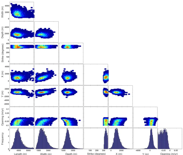
Table 2
A Priori Bounds and Inversion Results for a Horizontal Rectangular Source for the Observed Subsidence (From Leveling Surveys)
Length (m) Width (m) Depth (m) Strike (◦) Opening (cm/yr) X(m) Y(m)b
Lower bound 500 300 100 300 −10.0 −500 4,000
Upper bound 10,000 5,000 5,000 359 10.0 4,000 2,500
Optimala 3,516 1,939 1,377 321.2 −4.2 1,022 577.1
2.5% 1,338 1,838 958.7 302.1 −9.8 151.2 −1,302
97.5% 8,536 1,737 3,588 356.9 −1.5 2,436 1,610
Note. We give the optimal valuesa, and 2.5% and 97.5% percentile bounds of the posterior distributions (shown in
Figure 7).
aMaximum a posteriori probability bXand Y refer to the position in eastings and northings of the center of the
north-eastern edge of the sill relative to the reference point (124.641208◦E, 11.164502◦N). Opening is negative for a deflating source.
where p(m) is the prior PDF of the model parameters, which can be defined from a priori understanding of the physics of the problem (e.g., Bagnardi & Hooper, 2018; Jolivet, Simons, et al., 2015; Minson et al., 2013). For example, to model slip on the Philippine Fault, we can define prior PDFs that correspond to the known kinematics of the fault, that is, left-lateral strike slip. Cdis a variance-covariance matrix that describes the
noise in the data (as in Jolivet et al., 2012; Lohman & Simons, 2005; Sudhaus & Jónsson, 2009, among others). We then can sample models (m) to describe the posterior PDF and evaluate the model statistics (e.g., in terms of the mean and uncertainties of the PDF). We apply two different approaches to sample two different PDFs in the following sections, first to recover the geometry of the source of subsidence and then to derive the distribution of aseismic slip along the fault.
3.4.1. Inversion for the Subsidence Source Geometry
We used the subsidence measured from leveling surveys, done by Apuada et al. (2005) between 1997 and 2003, to infer the geometry of the underground source of subsidence. This allowed us to constrain the source geometry independently from the InSAR data and use the vertical velocity derived from InSAR as verifica-tion instead. We avoided inverting for the subsidence source geometry from the derived InSAR velocity maps as this might lead to parameter overfitting to the complex deformation field in the InSAR line-of-sight. We excluded the leveling data in the joint inversion of fault and subsidence deformation rates. As the raw level-ing data no longer exists, we digitized the subsidence contours from Apuada et al. (2005) and interpolated a raster of the subsidence rate using GRASS GIS (GRASS Development Team, 2017) (Figure 6a). Further, the elongated elliptical shape of the subsidence suggests a northwest trending source. We therefore inverted for a horizontal rectangular source (sill) in an elastic half-space (Okada, 1985) (Figure 6b and Table 2). We constrained the source parameters using the Geodetic Bayesian Inversion Software (GBIS; Bagnardi & Hooper, 2018). We determined the optimal source parameters, including length, width, depth, strike, position, and rate of opening. GBIS uses a Markov chain Monte Carlo (MCMC) sampling, controlled by a Metropolis-Hastings algorithm, to approximate the posterior PDF from the parameter space based on a priori assumptions of the source (Bagnardi & Hooper, 2018, and references therein). The prior PDFs are expressed as uniform probability density functions. As the subsidence source in Tongonan is unknown, we set broad bounds for the prior PDFs to allow exploration of different sill geometries between 0 and 5 km depth (a priori bounds are summarized in Table 2).
We generated 106samples of the posterior PDFs of the source parameters. The first 20,000 iterations of sampling, wherein the GBIS fine-tunes the ideal step size for the random walk in the parameter space for the succeeding samples (Bagnardi & Hooper, 2018), are excluded from the posterior PDFs. The maximum a posteriori probability is taken as the optimal solution from the whole distribution. For spatially continuous data (e.g., InSAR), GBIS also considers the uncertainties of the data in evaluating the posterior probability based on empirical estimation of variance and range (correlation distance) from semivariograms of the noise outside of deforming areas (e.g., Lohman & Simons, 2005; Sudhaus & Jónsson, 2009). As our subsidence data are spatially continuous but do not have far-field information, we arbitrarily assumed a variance (𝜎2) of 5 cm2/y2and a range (𝜆) of 1 km. The former is larger than the observed subsidence gradient (∼3 cm/yr), while the latter is smaller than the spatial extent of the data.
Figure 7. Posterior distribution and joint probabilities of subsidence source parameters from inversion with leveling data. Parameters include length, width,
depth, strike, position (X and Y ) relative to reference point, and rate of opening. Cooler colors correspond to lower frequency, and warmer colors indicate higher frequency. See Table 2 for the summary of the statistics of the inversion.
The results show an optimal sill geometry and negative opening (deflation) that largely captures the mag-nitude and pattern of subsidence (Figures 6). The observed subsidence can be explained by a northwest striking sill source at around 1.4 km depth from the surface, with deflation reaching 4.2 cm/yr (Table 2). The source depth coincides with the depth of the bottom of most wells in the Leyte geothermal production field (i.e., approximately between 1 and 2 km Apuada et al., 2005; Prioul et al., 2000, as displayed in supporting information Figure S6); hence, the probable depth of compaction that can result from geothermal fluid extraction (for a similar geothermal case in Iceland, see Receveur et al., 2019). Based on the joint marginals (Figure 7), we observe that the source geometry parameters are well constrained, with only a slight bias (or correlation) between the sill width and its location. The opening parameter negatively correlates with the width, length, and depth (between 1.2 and 2 km) of the source. The negative correlation between depth and opening means that a deeper source with a larger deflation could predict the observations on the surface as well as a shallower source with smaller deflation. Such bias is expected from the formulation of elastic dislocations and cannot be resolved with surface deformation data only. The fault-perpendicular profiles in Figure 6d show that the extent of the predicted subsidence is slightly wider than the observations, so the source might be slightly shallower. Nevertheless, we find that the extent of deformation and the location
Figure 8. Rate and extent of aseismic slip on the Philippine Fault in Leyte and model fit. (a) Mean of posterior PDF of aseismic slip, in cm/yr, with darker
colors indicating faster slip. Star: hypocenter of the July 2017 Mw6.5 earthquake. (b) Standard deviation of posterior PDF. (c–e) Downsampled ALOS ascending
Track 443 InSAR line-of-sight (LOS) velocity data, mean model prediction, and residuals. White square: extent of Figure 8, which shows fit of model to the data in Tongonan. Red line: faults included in model inversion. For the fit of model predictions to descending data, see supporting information Figure S8.
of the optimal model's predicted peak subsidence rate is similar to the vertical velocity component derived from the InSAR data (as shown by the red line and gray dots, respectively, in Profile S-S′, Figure 6d). The root-mean-square of the residuals (Figure 6c) is 0.2 cm/yr. These give us some confidence that the sill-like elastic subsidence source is a useful model to adopt for joint inversion with fault slip.
3.4.2. Fault Parametrization
We then defined the geometry of the fault in the joint inversion for aseismic slip and subsidence deforma-tion rate. Given the regional-scale strike-slip nature of the Philippine Fault, we assumed a vertical fault with the along-strike geometry based on existing active fault maps (Tsutsumi & Perez, 2013), modified to match the fault scarps and linear valleys observable from the 5-m resolution NAMRIA DEM. We reflected the left-stepping nature of the fault as two separate segments—the Northern Leyte and the Central Leyte Segments.
From 0 to 15 km depth, we divided the fault into rectangular patches with increasing patch sizes in three rows (see Figure 8 for the shallow fault geometry).
We explored different discretizations through qualitative trial-and-error tests (e.g., Sagiya & Thatcher, 1999), increasing the size variability from uniform 2 × 2 km square patches. We adopted the variable patch size
distribution that balances the ability to capture the heterogeneity at the shallowest sections of the fault (represented by smaller patches at the surface), the decreasing resolution with depth of inversion from sur-face data, and the convergence of the Bayesian sampling algorithm (Gombert et al., 2018; Jolivet, Simons, et al., 2015).
The downdip widths are 2 km on the top row, 5 km on the middle row, and 8 km on the bottom row. For the Northern Leyte Segment, the along-strike length from the top, middle, and bottom rows are 2, 10, and 30 km, respectively. We set slightly longer patches on the deeper rows of the Central Leyte Segment to account for the gaps in the surface data along the central highlands. The middle and bottom rows of the Central Leyte Segment have 12- and 40-km-long patches, respectively. At depths greater than 15 km, we introduced a single vertical fault with fewer but much larger patches to effectively mimic surface displacements related to an infinitely deep dislocation source, to capture deep slip below the seismogenic zone (Savage & Burford, 1973). Slip on the “deep” patch reflects the secular rate and predicts far-field displacements due to plate motion across a strike-slip boundary.
3.4.3. Joint Modeling of Aseismic Slip and Deflation From InSAR Data
We used AlTar (e.g., Gombert et al., 2018; Jolivet et al., 2014) to jointly solve for the PDF of slip on the fixed fault geometry and deflation rate on the subsidence source. AlTar is a parallel MCMC solver based on the early CATMIP algorithm (Minson et al., 2013) that benefits from GPU acceleration. This algorithm samples the parameter space, imposed by the prior PDF, using a Bayesian formalism. The sampling provides an ensemble of probable models that fit the data within its uncertainties. Furthermore, it does not involve any form of arbitrary smoothing of the solution, often used to regularize the inverse problem. Smoothing of slip between adjacent fault patches is usually a source of discrepancies between deterministic slip models (Duputel et al., 2015; Gombert et al., 2018; Minson et al., 2013, 2014).
We first downsampled the InSAR-derived surface deformation rates with a resolution-based algorithm (Lohman & Simons, 2005). We masked out points within 500 m from the fault to account for uncertainty in the geometry of the fault near the surface. Finally, we excluded data south of 10.6◦N where left-lateral slip is likely poorly resolved because the ascending track line-of-sight is orthogonal to the fault fault strike (as discussed in section 3.2). We used empirical exponential function fits to the noise covariograms of each InSAR data set to build the variance-covariance matrix (Cdin Equation 3), as in Jolivet et al. (2012). The empirical standard deviations and correlation lengths, respectively, were 0.1 cm/yr and 6 km for ascending Track 443, 0.2 cm/yr and 4 km for descending Track 76, and 0.3 cm/yr and 3 km for Descending Track 77. The covariograms are shown in supporting information Figure S7.
We assumed a uniform prior PDF for the deflation rate and slip parameters, reflecting our a priori under-standing of the left-lateral nature of the Philippine Fault. The fault patches at depths shallower than 15 km had a uniform prior PDF between −0.01 and 4 cm/yr, with positive values denoting left-lateral slip. The negative lower bound was set to allow efficient sampling of zero values. We assigned a normal (Gaussian) prior PDF to the deeper patches, with a mean of 3.0 cm/yr and a standard deviation of 0.25 cm/yr, to reflect the range of published farther-field and long-term slip rates (Barrier et al., 1991; Duquesnoy, 1997; Duquesnoy et al., 1994). As far-field displacement data (i.e., further than ∼20 km) is sparse, slip rate on the deeper patches may be less well constrained. Therefore, in order to speed up the sampling and to study only the distribution of aseismic slip consistent with current plate models, we used the Gaussian distribution with rather small standard deviation as the prior PDF.
We obtained more than 100,000 probable models that approximate the posterior PDF. For simplicity, in the following section, we primarily cite the mean and 1𝜎 of the posterior distribution of the parameters (the “mean model,” as shown in Figure 8), unless otherwise specified. The mode, skewness, and kurtosis of the posterior marginals (Figure 9) give us further indication of the robustness of inversion results as qualitative indicators of the “shape” of the posterior distribution.
3.5. Results: Variable Aseismic Slip Rate and Apparent Locked Section
The results of the modeling show varying rates of aseismic slip along-strike, with the mean model showing more than 3 cm/yr of slip on several section of the fault (Figure 8). The highest slip rates are present on the onshore Northern Leyte Segment and also along the shallowest patches of the Central Leyte Segment. Along most of the fault, between 2 and 15 km depth, most patches slip rapidly at around 2–3 cm/yr. The model also shows that, below 15 km depth, the fault slips at a rate of 3.3 ± 0.2 cm/yr. This rate is higher than the rates
Figure 9. (a) Mode, (b) skewness, and (c) kurtosis of the posterior distribution. (d) Resolution of the inversion on the
fault patches, with higher values indicating better resolution (see Appendix B for the resolution analysis).
from plate-scale kinematic analysis (2–2.5 cm/yr Barrier et al., 1991) but is similar to the rates derived from campaign GPS studies in Leyte (2.5–3.5 cm/yr; Duquesnoy et al., 1994; Duquesnoy, 1997).
In contrast, the southern end of the Northern Leyte Segment, hereafter referred to as the Tongonan Segment, appears to slip at a slower rate compared to the rest of the fault. Figure 8a shows that the aseismic slip rate on several contiguous patches from 0 to 7 km depth is close to 0. The small standard deviation (Figure 8b), as well as the mode, skewness, and kurtosis of the posterior PDF (Figure 9a to 9c) provide further indications of very low slip rate in Tongonan across the ensemble of probable models.
This reveals a previously unrecognized section of the fault that has a significant interseismic slip deficit, that is, a locked asperity, which can be a source of earthquakes. The depth of the hypocenter reported by
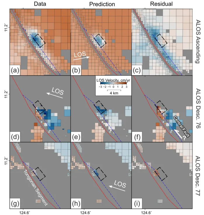
Figure 10. Downsampled InSAR LOS velocity data (left column), model prediction (middle column), and residuals (right column) in the Tongonan area, for
ALOS ascending Track 443 (top row, a–c), descending Track 76 (middle row, d–f), and descending Track 77 (bottom row, g–i). Red line: trace of the fault model. Dashed blue line: trace of the Tongonan Central Fault (Aurelio et al., 1993; Prioul et al., 2000). Dashed black rectangle: surface projection of the sill source. The residual velocity across the Tongonan Central Fault branch suggests that this fault is active. The opposite signs of LOS velocity between the ascending and descending tracks suggest that this is likely left-lateral deformation. See text for discussion (section 3.5).
the USGS for the July 2017 Mw6.5 earthquake is 9 ± 1.8 km, just at the bottom of the locked section (yellow
star in Figure 8a). PHIVOLCS, on the other hand, reports a depth of 2 km and a 6.5 surface magnitude (Ms)
(PHIVOLCS, 2017). We make further comparisons betweenthe interseismic and coseismic slip models for the July 2017 earthquakes (section 4) in the discussion (section 5).
The resolution matrix indicates that the inversion has resolving power on majority of the patches (Figure 9d, with details on the resolution analysis in Appendix B). The absence of any data points promixal to the shallowest sections of the fault where it goes underwater, in between Leyte and Biliran islands, have much poorer resolution than the patches that correspond to the onshore trace of the Philippine Fault.
(a)
(c)
(d)
(b)
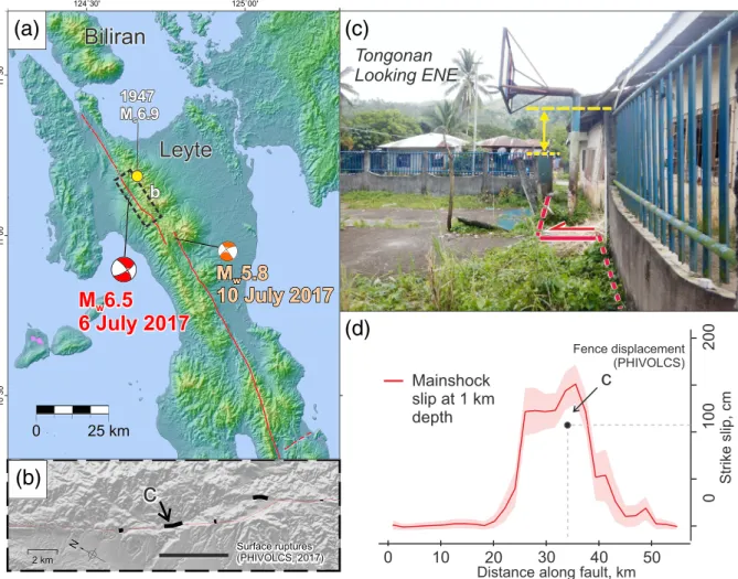
Figure 11. July 2017 earthquakes in Leyte. (a) Map showing the 6 July 2017 Mw6.5 mainshock (red) and 10 July 2017 Mw5.8 aftershock focal mechanisms,
obtained from the USGS website. Also shown for reference is the location of the 1947 Ms6.9 earthquake (yellow) from the ISC-GEM catalog (USGS, https://
earthquake.usgs.gov/earthquakes/eventpage/iscgem897883/executive). Dashed boxed indicates location of map in (b). (b) Surface ruptures mapped by PHIVOLCS (2017) quick-response team. (c) Displaced concrete fence near the village center of Tongonan, showing left-lateral displacement (red) with a vertical
component (yellow) associated with the July 2017 earthquakes, as reported by PHIVOLCS. (d) Along-strike variation of mean (red) and 1σrange (pink area) of
posterior strike-slip PDF at 1-km depth from the mainshock model (Figure 14). Distance, in km, is relative to the northern end of the fault in onshore Leyte. Reported displacement by PHIVOLCS (2017) of the fence shown for reference.
The far-field model predictions and residuals of LOS velocity show that our model largely captures the gradi-ent of fault deformation across Leyte (Figure 8d and 8e, respectively). The remaining residuals likely reflect uncorrected atmospheric noise or deformation that is not captured by a simple straight fault model in an elastic half-space.
Closer to the Philippine Fault in Tongonan, however, a linear pattern in residuals is visible, around 2 km east of the main fault trace (Figure 10). This probably is a manifestation of complexity in the deformation field in Tongonan that is not captured by the model. Our sill source model is in this area (dashed black rectangle in Figure 10) and has a deflation rate of 5.4 ± 0.4 cm/yr. This estimate appears to be well constrained as we do not observe obvious trade-offs between the joint marginal PDF of sill deflation and fault slip on adjacent patches (supporting information Figure S9). We, however, cannot exclude the possibilty of a more complex nature of vertical deformation, like subsidence controlled by minor faults. The residuals also might reflect aseismic slip on a secondary, parallel branch of the Philippine Fault—the Central Fault branch (Aurelio et al., 1993; Prioul et al., 2000) (Figure 10f). This seems to be a likely explanation as, when comparing Figure 10c and Figure 10f, the residual velocities between opposing line-of-sights are of different signs across the Central Fault, denoting horizontal motion. We explore this possibility and its implications in the discussion (section 5).
Table 3
Summary of Coseismic Interferograms Used in This Study
Event covered Date pair Satellite Track
M 2017/07/01-2017/07/07 Sentinel-1 61, Descending
A 2017/07/07-2017/07/13 Sentinel-1 61, Descending
M and A 2017/07/01-2017/07/13 Sentinel-1 61, Descending
M and A 2017/06/04-2017/07/15 ALOS-2 136, Descending
M and A 2016/02/13-2017/07/15 ALOS-2 24, Ascending
Note. M: Mainshock, A: Aftershock. Dates are formatted as yyyy/mm/dd.
4. Coseismic: 6 July 2017 M
w6.5 Mainshock and M
w5.8 Aftershock
The interseismic model of aseismic slip in Leyte suggests that the Tongonan section of the Philippine Fault could be locked. Following the 6 July 2017 Mw6.5 earthquake in Leyte, we thus evaluate any potential
over-lap between seismic and aseismic slip. The Mw6.5 event produced discontinuous surface ruptures, with
quick-response surveys by PHIVOLCS (2017) indicating that slip was distributed along the known traces of the fault in Tongonan (Figure 11). Offset of concrete structures show around a maximum of 1.1 m of left-lateral displacement, with around 0.6 m vertical displacement (Llamas et al., 2017) (Figure 11b). The earthquake was followed by several aftershocks, the largest of which (a Mw5.8 event) happened 4 days
later on 10 July 2017, with a similar strike-slip mechanism (orange “beach ball” in Figure 11a). No histori-cal earthquakes are known to have produced surface ruptures along this fault, although Besana and Ando (2005) suggest that earthquakes of magnitudes greater than 6.0 could have occurred in Leyte. More recently, Fukushima et al. (2019) highlight the similarity of the recorded waveforms of a Ms6.9 event in 1947 and the 2017 mainshock.
The recent published slip models of the 6 July 2017 mainshock have used interferograms that span both the mainshock and the aftershock (Fukushima et al., 2019; Yang et al., 2018). Hence, these slip distributions actually show the combined seismic slip from the 6 July mainshock and the 10 July aftershock. As listed in Table 3, there is a Sentinel-1 acquisition one day after the mainshock. We therefore propose to constrain the deformation from the mainshock and aftershock independently. However, only one Sentinel-1 acquisition was realized between the two events, so information is available for only one line-of-sight in constrain-ing the separate slip distributions of each event. ALOS-2, on the other hand, has only premainshock and postaftershock acquisitions, but data are available on both ascending and descending tracks. The modeling strategy we have developed to invert for the mainshock and aftershock slip distributions using all available interferograms (similar to Ragon et al., 2019) is described in the following section. This approach exploits the advantage of using different look geometries from distinct satellite tracks, providing more constraints to infer fault displacements.
4.1. Data and Methods 4.1.1. InSAR Data Processing
We used Sentinel-1 interferograms generated by the LiCSAR semiautomated processing chain (González et al., 2016). LiCSAR automatically combines bursts and subswaths of Sentinel-1 SLC images within predefined frames to create interferograms using GAMMA Software with minimal manual input. The inter-ferograms were multilooked by 20 and 4 in azimuth and range, respectively, roughly equivalent to pixels of around 60 m × 60 m pixels. We took the unfiltered interferograms from LiCSAR frame 061D_07906_131313 (derived from Sentinel-1 descending Track 61 data) that covers Leyte. In the processing, we included the NAMRIA IfSAR DEM (the same as in section 3.1) for topographic corrections and geocoding.
The ALOS-2 interferograms, as in Fukushima et al. (2019), were processed using the RINC software (Ozawa et al., 2016) with the SRTM1 DEM for topographic phase and geocoding. These interferograms were multilooked to an equivalent pixel size of 100 m × 100 m in range and azimuth.
We used an adaptive spectral filter on both data sets to increase the signal-to-noise ratio (Goldstein & Werner, 1998, as described in section 3.1). We unwrapped each interferogram with a region-growing branch-cut algo-rithm (i.e., grasses program in GAMMA). In order to reduce the occurrence of unwrapping errors in the
coseismic interferograms, we applied this method iteratively. We initially unwrapped regions with coher-ences above 0.8 and decreased the coherence threshold on each iteration. This step also flagged branch cuts to prevent unwrapping between pixels with sudden phase jumps, and then unwrapped small regions with high coherence. Succeeding iterations unwrapped areas with progressively lower coherence adjacent to the previously unwrapped regions. We manually checked for unwrapping errors at each iteration. Finally, from the result of the iteration with minimal unwrapping errors, we made manual corrections where nec-essary and masked any outstanding unwrapping errors that could not be corrected. For the Sentinel-1 interferograms, we did the filtering twice to make the unwrapping more efficient.
We estimated the noise covariance in each interferogram in regions where no coseismic deformation has been recorded, and downsampled the data for use in the inversion (both methods as described in section 3.4.3). The empirical standard deviation and correlation length of the Sentinel-1 coseismic data are ∼1.5 cm and ∼6 km, respectively. For the ALOS-2 data, these are ∼1 cm and 2 km, respectively. The covariance functions of the coseismic InSAR data sets can be found in supporting information Figure S10.
4.1.2. Inverting for Mainshock and Aftershock Slip
In order to obtain models of the mainshock and aftershock slip, we set up the inverse problem considering the different data sets (Table 3). The long temporal baseline of the ALOS-2 interferograms means that they include some interseismic (preseismic) and postseismic slip. For example, the premainshock acquisition of the ALOS-2 ascending Track 24 is almost 1.5 yr prior to the Mw6.5 event, which means that there could be
up to almost 6 cm of left-lateral displacement on sections that slip aseismically.
To separate the mainshock, aftershock, and preseismic and postseismic slips, we write the direct problem as
On the left-hand side, the d vector contains the five LOS displacement observations including only one or both of the mainshock- and aftershock-related signals (superscripts M and A, respectively), along either the ascending (subscript a) or descending (d) LOS from the ALOS-2 and Sentinel-1 satellites. The G matrix is a combination of Green's functions that relate slip on the fault from different source patches of the fault (m) to the observations in d. mMis the distribution of the mainshock coseismic slip, mAis the distribution of the
aftershock coseismic slip, and mPis the distribution of the sum of preseismic and postseismic slip recorded
by the ALOS-2 interferograms. We also include terms in G and m that allow us to fit a residual ramp for each individual data set.
We used the same fault parametrization of the Northern Leyte Segment as in the interseismic model (section 3.4.2), but use only the onshore patches. Our prior PDF is uniform for all strike-slip parameters, between −5 and 300 cm, and Gaussian for the dip-slip component (mean at 0 cm and the 3𝜎 probability range within −200 and 200 cm). Positive values of slip indicate left-lateral and reverse slip for strike slip and dip-slip, respectively.
As we also modeled the coseismic slip with AlTar, we primarily cite, in the following sections, the mean and standard deviation of the posterior PDF of slip, unless otherwise stated. We find that the mean and the mode of the posterior PDF are not significantly different (comparisons can be found in supporting information Figure S11). The fit of the model prediction to the observations are shown in supporting information Figure S12 for the Sentinel-1 data, and supporting information Figure S13 for the ALOS-2 data.
4.2. Results: Surface Deformation and Slip on the Fault
The interferograms clearly show the left-lateral deformation related to the Mw6.5 mainshock and the Mw5.8 aftershock. As respectively displayed in Figure 12 and Figure 13c, descending track Sentinel-1 and ALOS-2 interferograms show movement away from satellite LOS east of the fault, and displacement in the oppo-site sense on the west side. This is apparent despite poor coherence in the Sentinel-1 data near the fault.
Figure 12. Pairs of wrapped and unwrapped coseismic interferograms, from Sentinel-1 data, showing phase change and line-of-sight (LOS) displacement of
either the 6 July mainshock (Mw6.5) or the 10 July aftershock (Mw5.8), and their combined signal. Each map pair shows filtered wrapped interferogram (top)
and unwrapped displacement (bottom). Positive unwrapped LOS displacement indicates movement toward the satellite. Focal mechanisms of the earthquakes are included for reference. T: Tongonan. (a, d) Sentinel-1 descending Track 61 data, showing mainshock displacement only. (b, e) Same track, but showing aftershock displacement only. (c, f) Combined mainshock and aftershock displacement from Sentinel-1 descending Track 61.
In the ascending track ALOS-2 interferogram (Figure 13d), we note an opposite sign of LOS displacement compared to that in the descending track interferogram (Figure 13c). Thanks to the good coherence to the west of the fault in all interferograms, we can observe large LOS displacement right along the Tongonan Segment of the fault (white T in Figure 12d). This coincides with the location of the largest reported surface displacements in the field (Llamas et al., 2017; PHIVOLCS, 2017).
Comparing the Sentinel-1 wrapped interferograms that include the mainshock and the aftershock separately (Figures 12a and 12b, respectively) reveals that most of the deformation occurring during the aftershock hap-pened south of the mainshock. Discontinuities in the wrapped phase of both the mainshock and aftershock data appear to be on the same fault trace (the Tongonan Segment). For the aftershock, this discontinuity is just south of the fault bend. These observations strongly suggest that both seismic events ruptured the Tongonan Segment, but at different locations.
The model slip distributions in Figure 12 suggest that most of the seismic slip from both events occurred at depths shallower than 7 km. The largest magnitude of slip for the mainshock is confined within the upper 2 km of the fault, with up to 152 ± 21 cm of left-lateral slip (Figure 14a). This corresponds well with the location of the mapped surface ruptures in Tongonan (Figure 11a and 11b). The modeled strike-slip magnitude is only slightly higher than the observed field offsets (∼1.1 m, PHIVOLCS, 2017) (Figure 11c). Likewise, vertical displacements can also be observed in the field, with the eastern side downthrown by about 50 cm (PHIVOLCS, 2017) (Figure 11b). In our model, dip-slip of 27 ± 33 cm on the patch with the greatest slip reflects this but is not as well constrained as the strike slip (i.e., the standard deviation is larger than the mean). The discrepancies between the field observations and the model may be due to local ground conditions that can attenuate slip, and may also reflect limitations imposed by the size of the model's shallowest patches.
The aftershock model shows slip on fault patches directly south of the mainshock deformation, with a maximum slip of 36 ± 10 cm at depths between 2 and 7 km (Figure 14b). As similarly apparent in the inter-ferograms, it is notable that most of the aftershock slip is located just south of the fault bend. This may