HAL Id: insu-02998270
https://hal-insu.archives-ouvertes.fr/insu-02998270v2
Submitted on 4 May 2021
HAL is a multi-disciplinary open access
archive for the deposit and dissemination of
sci-entific research documents, whether they are
pub-lished or not. The documents may come from
teaching and research institutions in France or
abroad, or from public or private research centers.
L’archive ouverte pluridisciplinaire HAL, est
destinée au dépôt et à la diffusion de documents
scientifiques de niveau recherche, publiés ou non,
émanant des établissements d’enseignement et de
recherche français ou étrangers, des laboratoires
publics ou privés.
and liquid water cloud microphysical properties – Part
II: Results over oceans
Anne Garnier, Jacques Pelon, Nicolas Pascal, Mark Vaughan, Philippe
Dubuisson, Ping Yang, David Mitchell
To cite this version:
Anne Garnier, Jacques Pelon, Nicolas Pascal, Mark Vaughan, Philippe Dubuisson, et al.. Version 4
CALIPSO Imaging Infrared Radiometer ice and liquid water cloud microphysical properties – Part
II: Results over oceans. Atmospheric Measurement Techniques, European Geosciences Union, 2021,
pp.3277-3299. �10.5194/amt-14-3277-2021�. �insu-02998270v2�
https://doi.org/10.5194/amt-14-3277-2021 © Author(s) 2021. This work is distributed under the Creative Commons Attribution 4.0 License.
Version 4 CALIPSO Imaging Infrared Radiometer ice and liquid
water cloud microphysical properties – Part II: Results over oceans
Anne Garnier1, Jacques Pelon2, Nicolas Pascal3, Mark A. Vaughan4, Philippe Dubuisson5, Ping Yang6, andDavid L. Mitchell7
1Science Systems and Applications, Inc., Hampton, VA 23666, USA
2Laboratoire Atmosphères, Milieux, Observations Spatiales, Sorbonne University, Paris, 75252, France 3AERIS/ICARE Data and Services Center, Villeneuve-d’Ascq, 59650, France
4NASA Langley Research Center, Hampton, VA 23681, USA
5Laboratoire d’Optique Atmosphérique, Université de Lille, Villeneuve-d’Ascq, 59655, France 6Department of Atmospheric Sciences, Texas A&M University, College Station, TX 77843, USA 7Desert Research Institute, Reno, NV 89512, USA
Correspondence: Anne Garnier (anne.emilie.garnier@nasa.gov) Received: 25 September 2020 – Discussion started: 9 November 2020 Revised: 4 March 2021 – Accepted: 12 March 2021 – Published: 4 May 2021
Abstract. Following the release of the version 4 Cloud-Aerosol Lidar with Orthogonal Polarization (CALIOP) data products from Cloud-Aerosol Lidar and Infrared Pathfinder Satellite Observations (CALIPSO) mission, a new version 4 (V4) of the CALIPSO Imaging Infrared Radiometer (IIR) Level 2 data products has been developed. The IIR Level 2 data products include cloud effective emissivities and cloud microphysical properties such as effective diameter (De) and
water path estimates for ice and liquid clouds. This paper (Part II) shows retrievals over ocean and describes the im-provements made with respect to version 3 (V3) as a re-sult of the significant changes implemented in the V4 algo-rithms, which are presented in a companion paper (Part I). The analysis of the three-channel IIR observations (08.65, 10.6, and 12.05 µm) is informed by the scene classification provided in the V4 CALIOP 5 km cloud layer and aerosol layer products. Thanks to the reduction of inter-channel ef-fective emissivity biases in semi-transparent (ST) clouds when the oceanic background radiance is derived from model computations, the number of unbiased emissivity retrievals is increased by a factor of 3 in V4. In V3, these biases caused inconsistencies between the effective diameters re-trieved from the 12/10 (βeff12/10 = τa,12/τa,10) and 12/08
(βeff12/08 = τa,12/τa,08) pairs of channels at emissivities
smaller than 0.5. In V4, microphysical retrievals in ST ice clouds are possible in more than 80 % of the pixels down to
effective emissivities of 0.05 (or visible optical depth ∼ 0.1). For the month of January 2008, which was chosen to illus-trate the results, median ice De and ice water path (IWP)
are, respectively, 38 µm and 3 g m−2in ST clouds, with ran-dom uncertainty estimates of 50 %. The relationship between the V4 IIR 12/10 and 12/08 microphysical indices is in better agreement with the “severely roughened single col-umn” ice habit model than with the “severely roughened eight-element aggregate” model for 80 % of the pixels in the coldest clouds (<210 K) and 60 % in the warmest clouds (>230 K). Retrievals in opaque ice clouds are improved in V4, especially at night and for 12/10 pair of channels, due to corrections of the V3 radiative temperature estimates de-rived from CALIOP geometric altitudes. Median ice Deand
IWP are 58 µm and 97 g m−2at night in opaque clouds, with again random uncertainty estimates of 50 %. Comparisons of ice retrievals with Moderate Resolution Imaging Spec-troradiometer (MODIS)/Aqua in the tropics show a better agreement of IIR Dewith MODIS visible–3.7 µm than with
MODIS visible–2.1 µm in the coldest ST clouds and the op-posite for opaque clouds. In prevailingly supercooled liquid water clouds with centroid altitudes above 4 km, retrieved median De and liquid water path are 13 µm and 3.4 g m−2
in ST clouds, with estimated random uncertainties of 45 % and 35 %, respectively. In opaque liquid clouds, these values are 18 µm and 31 g m−2 at night, with estimated
uncertain-ties of 50 %. IIR Dein opaque liquid clouds is smaller than
MODIS visible–2.1 µm and visible–3.7 µm by 8 and 3 µm, respectively.
1 Introduction
The Imaging Infrared Radiometer (IIR) is one of the three instruments on board the Cloud-Aerosol Lidar and Infrared Pathfinder Satellite Observations (CALIPSO) satellite which has been in quasi-continuous operation since mid-June 2006 (Winker et al., 2010). IIR is co-aligned with Cloud-Aerosol Lidar with Orthogonal Polarization (CALIOP) and with the Wide Field Camera (WFC), which are all arranged in a star-ing, near-nadir-looking configuration. The IIR instrument in-cludes three medium resolution channels in the atmospheric window centered at 08.65, 10.6, and 12.05 µm with 1 km2 pixel size. Geolocated and calibrated radiances for all chan-nels are reported in IIR Level 1 products. The IIR Level 2 data products include clouds effective emissivities and cloud microphysical properties such as effective diameters and ice or liquid water path estimates. Following the release of the version 2 IIR Level 1 products (Garnier et al., 2018) and of the version 4 (V4) CALIOP data products, a new version 4 (V4) of the IIR Level 2 data products has been developed and is now available publicly.
The V4 algorithm and its changes with respect to version 3 (V3) are presented in a companion paper (Garnier et al., 2021, hereafter “Part I”). Cloud microphysical properties are derived using the split-window method relying on the analy-sis of inter-channel effective absorption optical depth ratios, or microphysical indices, from which effective diameter is inferred. The concept of the microphysical index was intro-duced by Parol et al. (1991) and has been widely used for op-erational retrievals (Heidinger and Pavolonis, 2009; Pavolo-nis, 2010). Ice cloud absorption is stronger at 12.05 µm than at 10.6 µm or 08.65 µm. As a result, the brightness temper-atures are smaller at 12.05 µm; hence, a well-known split-window retrieval approach is used in the analysis of inter-channel brightness temperature differences (Inoue, 1985). Hyperspectral infrared sensors such as Atmospheric Infrared Sounder (AIRS) or Infrared Atmospheric Sounder Interfer-ometer (IASI) allow advanced multi-channel analyses using optimization techniques (Kahn et al., 2014) and the analy-sis of the spectral coherence of the retrieved cloud emissiv-ities (Stubenrauch et al., 2017). The split-window technique in the thermal infrared spectral domain is very sensitive to the presence of small particles having a maximum dimen-sion smaller than approximately 50 µm in the size distribu-tion (Mitchell et al., 2010). It was shown using the Mod-erate Resolution Imaging Spectroradiometer (MODIS) ther-mal infrared bands that observations in this spectral domain are perfectly suited to unambiguously identify the presence of small ice crystals in cold cirrus clouds (Cooper and
Gar-rett, 2010). As such, thermal infrared techniques can provide insights into the observations of small crystals by some in situ instruments when measurements of sizes smaller than 15 µm are uncertain (Mitchell et al., 2018) and help evaluate the possible effects of crystal shattering (Cooper and Garrett, 2011).
Regardless of the retrieval approach, the split-window technique is best adapted for retrievals in clouds of medium effective emissivity. Uncertainties are minimum for cloud effective emissivities between 0.2 and 0.9 (Garnier et al., 2013, hereafter G13), or cloud optical depth between about 0.45 and 4.6, where the information content is the largest (Iwabuchi et al., 2014; Wang et al., 2016). Given sufficiently accurate emissivity estimates, retrievals of cloud properties beyond these lower and upper limits remain possible un-til the emissivities are either too close to 0 for subvisible clouds or too close to 1 for clouds behaving as blackbody sources, at which points the technique totally loses sensitiv-ity. In addition, the logarithmic relationship between cloud optical depth and infrared emissivity causes a saturation of the cloud optical depths retrievals. For instance, emissivities larger than 0.99 correspond to cloud optical depth larger than only 9. Techniques relying on the combination of visible and near-infrared bands, as used in MODIS operational retrievals (Nakajima and King, 1990; Platnick et al., 2017), are bet-ter suited than thermal infrared techniques for cloud optical depths larger than 5 (Wang et al., 2011), but these methods are limited to daytime observations only.
Due to its sensitivity to small particles, the split-window technique is an attractive option for retrievals of liquid droplet sizes (Rathke and Fisher, 2000), and microphysical retrievals in liquid water clouds are now included in the V4 IIR products. All other things being equal, the performance of the split-window technique increases with the radiative contrast between the cloud and the surface. Consequently, re-trieval uncertainties are larger for liquid water clouds, which typically form relatively close to the Earth’s surface, and hence these retrievals were not included in V3. Liquid wa-ter clouds such as marine stratocumulus clouds, which are an important component of the Earth system, have optical depths typically larger than 10, well beyond the range of ap-plicability of the technique. However, infrared observations have the potential to provide new insight into the microphysi-cal properties of thin liquid water clouds (Turner et al., 2007; Marke et al., 2016) and supercooled mid-level liquid water clouds.
The IIR analyses start with the retrieval of cloud effec-tive emissivities in each channel, which are then converted to effective absorption optical depths as τa,k= −ln(1 − εeff,k),
where εeff,08, εeff,10, and εeff,12 are the effective emissivities
retrieved in IIR channels 08.65 (k = 08), 10.6 (k = 10), and 12.05 (k = 12), respectively. Effective emissivity is mostly a measure of cloud absorption, and the term “effective” refers to the contribution from scattering, which is the most significant at 08.65 µm. The first IIR microphysical index,
βeff12/10 = τa,12/τa,10, is the ratio of the effective
absorp-tion optical depths at 12.05 and 10.6 µm and the second one, βeff12/08 = τa,12/τa,08, is the ratio of the effective
absorp-tion optical depths at 12.05 and 08.65 µm. Two main pieces of information are needed to retrieve these quantities: the cloud top-of-atmosphere (TOA) blackbody radiance, which requires a good estimate of the cloud radiative temperature, and the TOA background radiance that would be observed if no cloud were present. The former drives the accuracy at large emissivities and the latter the accuracy at small emis-sivities.
The first step into any retrieval approach is the detec-tion of a cloud and the determinadetec-tion of its thermodynamic phase and radiative temperature. The ability to ascertain cloud amounts and characteristics varies with the observ-ing capabilities of different passive sensors (Stubenrauch et al., 2013). Even though IIR has only three medium resolu-tion channels, its crucial advantage is the quasi-perfect co-location with CALIOP observations. Indeed, as emphasized by Cooper et al. (2003), cloud boundaries measured by ac-tive instruments provide an invaluable piece of information for obtaining accurate estimates of cloud radiative tempera-tures. The IIR algorithm relies on CALIOP’s highly sensitive layer detection to characterize the atmospheric column seen by each IIR pixel. CALIOP provides geometrical altitudes which are converted into radiative temperatures. The radia-tive temperature, Tr, of a multi-layer cloud system is
esti-mated as the thermodynamic temperature, Tc, at the centroid
altitude of the CALIOP attenuated backscatter at 532 nm. In the V4 algorithm, this estimate is further corrected when single- or multi-layer ice cloud systems are observed (Part I). The thermodynamic temperature is derived from interpo-lated temperatures profiles of the Global Modeling and As-similation Office (GMAO) Modern-Era Retrospective anal-ysis for Research and Applications version 2 (MERRA-2) model (Gelaro et al., 2017).
The second retrieval step is the determination of the TOA background radiance, which often requires simulations us-ing ancillary meteorological profiles and surface data. These simulations are generally more accurate over oceans than over land because the surface emissivities in the various channels are better known and less variable over oceans, and the skin temperature data are usually more accurate. In this paper, we therefore focus on retrievals over oceans. In the IIR algorithm, the TOA background radiance is preferentially de-termined using observations in neighboring pixels in those cases when clear-sky conditions, as determined by CALIOP, can be found. Otherwise, it is computed using the fast-calculation radiative transfer (FASRAD) model (Garnier et al., 2012; Dubuisson et al., 2005). In V3, IIR microphysical retrievals over oceans were possible down to εeff,12∼0.05
(or optical depth ∼ 0.1) when the background radiance could be measured in neighboring pixels (G13). When the back-ground radiance had to be computed by FASRAD, which represents about 75 % of the cases, inter-channel biases in
the model simulations caused discernable flaws in the micro-physical retrievals. The inter-channel biases in the FASRAD simulations have been significantly reduced in V4, as dis-cussed in Part I.
This paper aims at demonstrating the improved accuracy of the V4 effective emissivities and of the subsequent micro-physical indices that result from the changes implemented in the V4 algorithm (Part I) and at illustrating the changes in the retrieved microphysical properties. Our assessment is carried out after carefully selecting the relevant cloudy scenes, fol-lowing the rationale presented in Sect. 2. Retrievals in ice clouds are presented in Sect. 3, which includes step-by-step comparisons between V3 and V4, examples of V4 retrievals, and comparisons with MODIS retrievals. Section 4 is dedi-cated to retrievals in liquid water clouds that were added in V4, and Sect. 5 concludes the presentation.
2 Cloudy scene selection
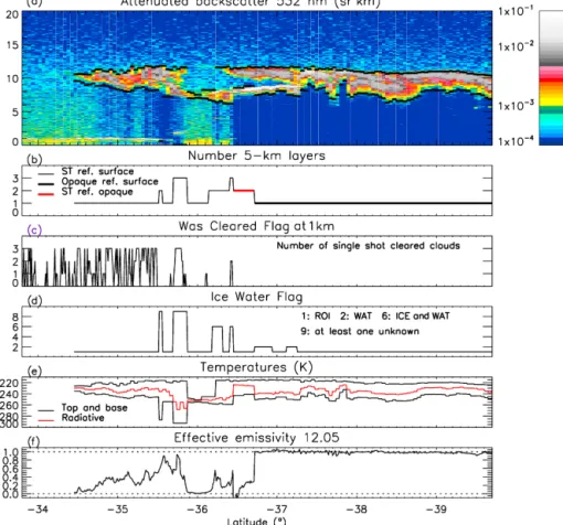
The analysis of the IIR observations is informed by the scene classification provided by the V4 CALIOP cloud and aerosol 5 km layer products. This scene classification is established for layers detected by the CALIOP algorithm at 5 and 20 km horizontal averaging intervals (Vaughan et al., 2009). An ex-ample is shown in Fig. 1, which was extracted from nighttime granule 2008-01-30T09-15-45ZN on 30 January 2008.
Figure 1a shows the Level 1 CALIOP attenuated backscat-ter averaged at 5 km horizontal resolution with the top and base altitudes of the cloud system shown in black. Cloudy scenes can include one or several layers (Fig. 1b). When the lowest of at least two layers is opaque to CALIOP, this opaque layer is used as a reference assuming it behaves as a blackbody source and the algorithm retrieves the properties of the overlying semi-transparent (ST) layers. An example is found between latitudes −36.45 and −36.7◦, highlighted in red in Fig. 1b, where the algorithm retrieves the proper-ties of two ST layers overlying the opaque cloud located at about 8 km altitude. South of −36.7 and down to −37.2◦, the portion of this cloud which is used as an opaque ref-erence between −36.45 and −36.7◦ is included in a single opaque cloud of top altitude equal to 11.5 km, which ex-tends down to the southernmost latitudes. North of −36.45 and up to −34.45◦, the atmospheric column includes one to three semi-transparent clouds. Finally, no cloud layers are seen north of −34.45◦, where the scenes contain only low ST non-depolarizing aerosol layers (not shown). The atmo-spheric column might also contain clouds having top alti-tudes lower than 4 km that are detected at single-shot reso-lution and then cleared before searching for the more tenu-ous layers typically reported in the 5 km products (Vaughan et al., 2009). These single-shot detections are not included in Fig. 1b. The number of these single-shot cleared clouds seen within each IIR pixel is shown in Fig. 1c. We showed in Part I (Fig. 5 in Part I) that the presence of these cleared clouds
Figure 1. Example of the CALIOP scene classification information used for effective emissivity retrievals on 30 January 2008 (granule 2008-01-30T09-15-45ZN). (a) CALIOP attenuated backscatter with top and base altitudes of the cloud system highlighted in black; (b) number of cloud layers in the cloud system; cases with Earth surface as a reference are denoted with black lines (thin: semi-transparent (ST) layers; thick: one opaque layer), and in red are the cases with the lowest opaque cloud as a reference; (c) CALIOP “Was Cleared” flag at 1 km IIR pixel resolution; (d) ice water flag of the cloud system; (e) temperatures at cloud top and cloud base (black) and radiative temperature used by the IIR algorithm (red); (f) effective emissivity of the cloud system at 12.05 µm. See text for details.
modifies the background radiance compared to the radiance due to the ocean surface and ultimately biases the effective emissivity retrievals. Because these biases cannot be quan-tified a priori, scenes that contain single-shot cleared clouds should be treated with caution. The ice water flag shown in Fig. 1d characterizes the ice–water phase of the cloud layers included in the cloud system. These layers are classified ei-ther as ice, liquid water, or “unknown” by the V4 CALIOP ice–water phase algorithm (Avery et al., 2020). Most of the ice clouds are composed of randomly oriented ice (ROI) crystals. Clouds containing significant fractions of horizon-tally oriented ice (HOI) crystals are also detected, mainly be-fore the end of November 2007, when the platform tilt angle was changed from its initial 0.3◦orientation to a view angle of 3◦(Avery et al., 2020). In Fig. 1, we find cloud systems composed of ROI only (flag = 1), liquid water (WAT) only (flag = 2), ice and WAT (flag = 6), and some systems that in-clude at least one layer of unknown phase (flag = 9). IIR ef-fective emissivities are reported for all single- or multi-layer scenes, regardless of the phase. In V4, the phase
informa-tion is used to adjust the radiative temperature (Fig. 1e) esti-mates in cases containing ice clouds (Part I). For illustration purposes, the V4 retrieved effective emissivities at 12.05 µm are shown in Fig. 1f. In this example, emissivity values in the opaque cloud are mostly around 1, the lowest value be-ing 0.91 at −39.5◦ where the CALIOP image suggests the presence of a faint signal below the cloud. Effective emissiv-ities in ST clouds vary between 0 and 0.9. The only excep-tion is between −36.45 and −36.52◦, where non-physical negative effective emissivities are retrieved because the com-puted background radiances are smaller than the observed radiances and are therefore underestimated. In this case, the reference is a cloud classified as opaque by CALIOP (see area highlighted in red in Fig. 1b), which is likely not suffi-ciently dense to behave as a blackbody reference.
This example shows that a cloudy scene can include a vari-ety of conditions for the IIR retrievals. Because the goal here is to present the cloud microphysical properties as retrieved with the IIR V4 algorithm and improvements with respect to V3, we chose to limit the analyses to scenes that contain
only ROIs, only HOIs, or only WAT clouds with background radiances from the ocean surface. Furthermore, in order to facilitate the interpretation of the results, we require that the CALIOP cloud–aerosol discrimination algorithm (Liu et al., 2019) assign high confidence to the cloud classifications and likewise that the ice–water phase algorithm determined the phase classifications with high confidence. Finally, scenes containing single-shot cleared clouds are discarded. Table 1 reports the fraction of scenes that fall into these categories. The statistics are for IIR pixels between 60◦S and 60◦N in January and July 2008. The ROI scenes represent 13 % to 16 % of all the IIR pixels. The HOI scenes represent less than 0.1 % of all the IIR pixels, and we found that they represent less than 1 % at the beginning of the mission when the plat-form tilt angle was 0.3◦. Thus, in the rest of the paper, ice clouds will refer to scenes containing only ROI layers. The WAT scenes represent 14 % to 19 % of all the IIR pixels.
Clear-sky conditions are defined as cloud-free scenes with the “Was Cleared” flag at 1 km resolution equal to zero, with no aerosol layers or only low (<7 km) semi-transparent “not dusty” layers. Dusty layers are those identified as dust, pol-luted dust, or dusty marine (Kim et al., 2018) and are dis-carded because they may have a signature in the IIR channels (Chen et al., 2010). For comparison with the previous cate-gories, the clear-sky conditions represent 20 % of the cases for daytime data and 15 % for nighttime data. It is noted that 6 % to 10 % of the pixels are rejected as “clear sky” in V4 due to the presence of single-shot cleared clouds. These pix-els would have been accepted by the V3 algorithm: they rep-resent 25 % and 35 % of the V3 clear-sky conditions for day-time and nightday-time data, respectively.
Scenes composed of only high-confidence ROI layers or only WAT layers can include either one opaque layer or a number of ST layers. This is quantified in Table 2 for the months of January and July 2008. For these months, 45 to 53 % of the selected ROIs are opaque to CALIOP, while opaque clouds represent 67 % to 90 % of the WATs. Daytime fractions of opaque clouds are larger than nighttime ones, which is likely due daytime surface detection issues. Scenes with only ST layers are spread into three main categories: only one layer, two vertically overlapping layers detected at different horizontal averaging resolutions where the top alti-tude of the lower layer is greater than the base altialti-tude of the higher layer, and multi-layer configurations with two non-overlapping layers or more than two layers. For both ROI and WAT clouds, the vast majority of the ST scenes have only one layer in the column, which is explained by the fact that we required all the layers to be characterized with high con-fidence. Thus, the study will be carried out for single-layer cases for simplicity.
3 Retrievals in ice clouds
The accuracy of the effective emissivity in each IIR channel and of the subsequent microphysical indices is a prerequi-site for successful retrievals of cloud microphysical proper-ties. In Sect. 3.1, we use internal quality criteria to demon-strate the improvements in the V4 effective emissivities in ice clouds that result from the revised computed background radiances over oceans and from the revised radiative tem-perature estimates (Part I). After examining the changes in εeff,12 (at 12.05 µm), inter-channel effective emissivity
dif-ferences, 1εeff12 − k = εeff,12−εeff,k, are assessed, keeping
in mind that they should tend towards zero on average when εeff,12 tends towards 0 and towards 1 (G13; Part I). Changes
in the visible cloud optical depth, τvis, inferred from the
sum-mation of absorption optical depths at 12.05 µm and 10.6 µm (τa,12+τa,10; Part I), are shown in Sect. 3.2.
The subsequent improvements in the microphysical in-dices and in the performance of the microphysical algorithm are discussed in Sect. 3.3, where we also illustrate changes in the effective diameters (De) reported in V3 and V4. We recall
that Deis defined as De=(3/2) × (V /A), where V is the
to-tal volume of the size distribution and A is the corresponding projected area (Foot, 1988; Mitchell, 2002). The V4 algo-rithm uses two ice habit models from the “TAMUice2016” database (Bi and Yang, 2017; Yang et al., 2013), namely the severely roughened solid column (SCO) and severely rough-ened eight-element column aggregate (CO8) models, and the model used for the retrievals is selected according to the re-lationship between βeff12/10 and βeff12/08. IIR retrieved
De is the mean of the De12/10 and De12/08 effective
di-ameters when these two values can be retrieved from the respective βeff12/ k; that is, De= (De12/10 + De12/08) /2.
Both De12/10 and De12/08 are reported in the product for
users interested in specific analyses. The V4 look-up tables (LUTs) that relate microphysical index and effective diam-eter are computed using the fast discrete ordinate method (FASDOM) (Dubuisson et al., 2008) model and bulk single scattering properties derived using an idealized gamma par-ticle size distribution. In V3, the LUTs were derived using single scattering properties of the “solid column” and “aggre-gate” ice habit models from the database described in Yang et al. (2005), with no particle size distribution. We showed in Part I that, everything else being equal, the size distribution introduced in V4 increases retrieved De. As illustrated in Part
I, the microphysical indices are very sensitive to Desmaller
than 50 µm and the sensitivity decreases progressively up to De=120 µm, which is considered the sensitivity limit of our
retrievals in ice clouds.
In Sect. 3.4, we show examples of V4 De and ice water
path (IWP) microphysical retrievals and comparisons with MODIS retrievals are presented in Sect. 3.5.
Table 1. Total number of IIR pixels, fraction of IIR pixels with only high-confidence ROI, WAT, and HOI layers in the column and no single-shot cleared clouds for retrievals with background radiance from the ocean surface between 60◦S and 60◦N, and fraction of clear-sky pixels.
January 2008 July 2008 Night Day Night Day No. of IIR pixels 4.2 × 10⁶ 4.2 × 10⁶ 3.8 × 10⁶ 3.9 × 10⁶
Fraction of IIR pixels
ROI 0.132 0.160 0.127 0.155 HOI <0.001 <0.001 <0.001 <0.001 WAT 0.175 0.192 0.143 0.182 Clear sky 0.143 0.204 0.165 0.208 Clear sky rejected in V4 0.083 0.063 0.097 0.074
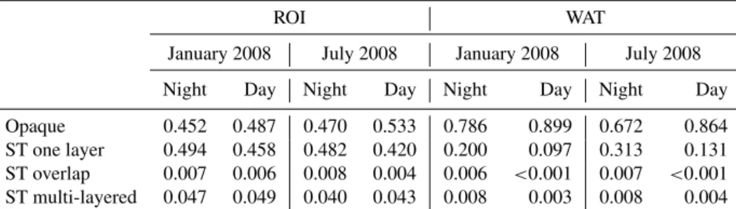
Table 2. Detailed statistics for IIR pixels with only ROI or WAT high-confidence layer(s) in the column and no cleared clouds for retrievals with background radiance from the ocean surface between 60◦S and 60◦N in January and July 2008: fraction of opaque clouds, single-layered ST clouds, ST clouds with two overlapping layers, and multi-single-layered ST clouds.
ROI WAT
January 2008 July 2008 January 2008 July 2008 Night Day Night Day Night Day Night Day Opaque 0.452 0.487 0.470 0.533 0.786 0.899 0.672 0.864 ST one layer 0.494 0.458 0.482 0.420 0.200 0.097 0.313 0.131 ST overlap 0.007 0.006 0.008 0.004 0.006 <0.001 0.007 <0.001 ST multi-layered 0.047 0.049 0.040 0.043 0.008 0.003 0.008 0.004
3.1 Effective emissivity: V4 vs. V3
Because of numerous changes in the CALIOP V4 algo-rithms, the cloud layers reported in the V3 and V4 CALIOP data products are not identical, so direct comparisons of the V3 and V4 IIR data products could be misleading. In order to isolate the changes due to the IIR algorithm, the V3 emissivi-ties (hereafter V3_comp) for clouds reported in CALIOP V4 were recomputed using the V3 computed background radi-ances reported in the V3 product and the V3-like blackbody temperatures derived directly from the centroid temperatures, Tc, which are available in the V4 product along with the V4
blackbody temperatures. The exercise was carried out for V4 scenes over oceans that contain a single cloud layer classified as high-confidence ROI with no cleared clouds, as discussed previously in Sect. 2. Illustrations are shown for the month of January 2008 between 60◦S and 60◦N.
3.1.1 Effective emissivity in channel 12.05
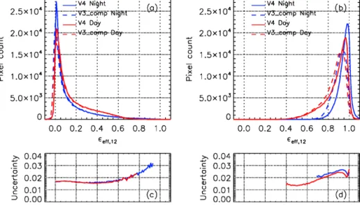
The nighttime (blue) and daytime (red) distributions of εeff,12
are shown in Fig. 2, where V4 (solid lines) is compared with V3_comp (dashed lines). Figure 2a and b show the distribu-tions for ST and opaque clouds, respectively. The V4 median random uncertainty estimates shown in Fig. 2c and d are of
the order of 0.015 at εeff,12<0.6 and increase up to 0.03 at the
largest emissivities, where the uncertainty in εeff,12is
prevail-ingly due to the uncertainty in the radiative temperature taken equal to ±2 K (Part I). Because of retrieval errors, εeff,12can
be found outside the range of physically possible values (i.e., 0 to 1). For ST clouds (Fig. 2a), the V3 and the V4 histograms differ mostly at εeff,12<0.05, where the changes in the
back-ground radiances have the largest impact. In this example, the fraction of ST clouds with negative εeff,12values is reduced
from 12 % in V3 to 3.5 % in V4. For opaque clouds (Fig. 2b), the larger V4 εeff,12 values are due to the radiative
tem-perature corrections introduced in the V4 algorithm (these corrections have essentially no impact on ST clouds). For the range of εeff,12 values found in opaque clouds, the
cor-rections are prevailingly a function of the “apparent” cloud thickness, which is larger and closer to the true geometric thickness at night (Part I). Nighttime and daytime εeff,12
dis-tributions peak at larger εeff,12in V4 (εeff,12=0.99 and 0.97,
respectively) than in V3 (εeff,12=0.94). Consequently,
ran-dom uncertainties and possible overcorrections cause an in-crease of the fraction of samples with εeff,12>1, from 3 %
in V3 to 12 % in V4 at night, and from 1.2 % to 3.3 % for daytime data. At night, 98 % of the opaque clouds have V4 εeff,12>0.8 or cloud optical depth >3.2. This lower range of
retrievals, even though it is recognized that direct compar-isons with V4 CALIOP optical depths in opaque clouds are difficult (Young et al., 2018). Nighttime εeff,12distributions
for ST and opaque clouds are essentially mutually exclusive, with a εeff,12 threshold around 0.7. In contrast, these
distri-butions overlap between 0.4 and 0.7 for daytime data. The tail down to εeff,12=0.4 (τvis∼1) for daytime opaque cloud
data is explained by a greater difficulty for the CALIOP al-gorithm to detect faint surface echoes during the day due to large solar background noise, so some clouds of moder-ate emissivity may be misclassified as opaque by CALIOP. Effective emissivities close to 1 are found in clouds where the CALIOP integrated attenuated backscatter (IAB) is larger than 0.04 sr−1, which is in the upper range of values typically observed in opaque ice clouds (Young et al., 2018). Platt et al. (2011) showed that these large IABs, which are often coupled with small apparent geometric thicknesses, are ob-served when the CALIPSO overpass is close to the center of a mesoscale convective system. Using cloud retrievals based on AIRS thermal infrared data, Protopapadaki et al. (2017) demonstrated that emissivities close to 1 in the tropics are most often indicative of convection cores reaching the up-per troposphere, which confirms our observations based on CALIPSO.
3.1.2 Inter-channel effective emissivity differences We recall that effective emissivity retrievals preferably use background radiances observed in neighboring clear-sky pix-els and otherwise use radiances computed by FASRAD. In order to evaluate V4 computed background radiances, we first examined 1εeff12 − k at εeff,12∼0 in ST clouds by
sep-arating retrievals that used observed radiances (V4_obs) and those that used computed radiances (V4_comp). The results are reported in Table 3, where 1εeff12 − k at εeff,12≈0 is
also reported for V3_comp for reference. As in V3 (G13), V4 inter-channel biases are minimum when the background radiance can be determined from observations (V4_obs), which represents 30 % of the retrievals in ST clouds for this dataset. When the background radiance is computed (V4_comp, 70 % of the cases), median 1εeff12 − k is similar
for both channel pairs and smaller than 0.0025 in absolute value. This indicates residual inter-channel biases smaller than 0.1 K in V4 according to the simulations shown in Fig. 1b of Part I, which is consistent with the residual inter-channel differences seen in clear-sky conditions (Part I). Be-cause these biases are very small, retrievals using computed and observed radiances are consistent in V4, and hereafter the two methods will be referred to collectively as “V4” for clarity. The 1εeff12 − k differences were unambiguously too
low in V3_comp, especially for the 12–08 pair, so reliable retrievals were possible only when observed radiances were available (G13). Including retrievals using computed radi-ances in V4 increases the number of retrievals in ST clouds by a factor of 3.3.
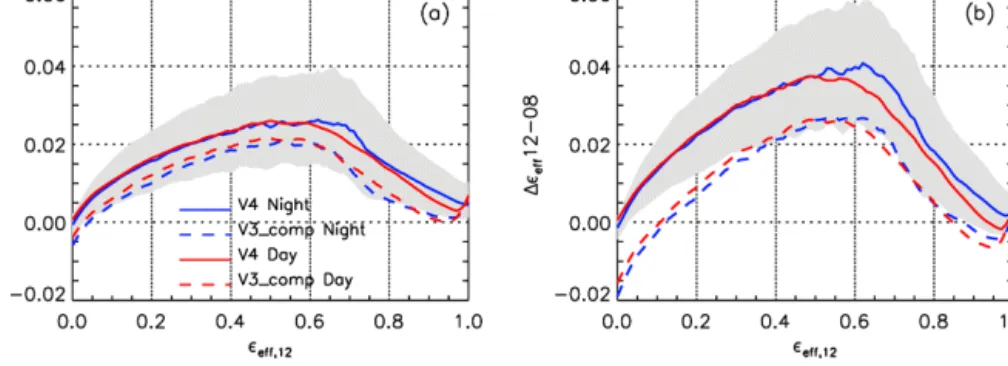
The variations with εeff,12of the 1εeff12 − k inter-channel
effective emissivity differences for the 12–10 and 12–08 pairs are shown in Fig. 3a and b, respectively. The curves are median values, and the shaded gray areas are between the V4 nighttime 25th and 75th percentiles. The first observation is that median 1εeff12 − k are larger in V4 (solid lines) than in
V3_comp (dashed lines) at any emissivity. When εeff,12tends
towards 1, 1εeff12−k is minimum at εeff,12corresponding to
the peak of the distributions shown in Fig. 2, which suggests that the peaks should be closer to εeff,12=1. This shows
that V4 is improved compared to V3, more convincingly for nighttime data, but also that the radiative temperature correc-tions are likely not sufficient. Consistent with the simulacorrec-tions shown in Fig. 1 of Part I, 1εeff12 − k are increased from V3
to V4 at large emissivities, because the radiative tempera-tures are increased, and the changes are more important in the 12/08 pair than in the 12/10 pair.
3.2 Visible cloud optical depth: V4 vs. V3
The V3–V4 changes in the visible cloud optical depths in-ferred from εeff,12 and εeff,10 are shown in Fig. 4a and b
for nighttime and daytime data, respectively. The large plots where τvisranges between 0 and 15 are built using bins equal
to 0.2, and the small embedded plots show details for τvis
smaller than 1 and bins equal to 0.02. The changes in τvis
are smaller than 0.02 on average and not significant for τvis
smaller than 2 (or εeff,12< ∼0.6), that is for most of the ST
clouds. For τvis>2, V4 τvis is increasingly larger than V3
τvis, due to the warmer radiative temperature estimates in V4.
Consistent with previous observations regarding εeff,12, the
τvis increase from V3 to V4 is larger at night (Fig. 4a) than
during the day (Fig. 4b).
3.3 Microphysical indices and effective diameter retrievals: V4 vs. V3
The changes in the βeff12/10 and βeff12/08
microphysi-cal indices resulting from the changes in 1εeff12–10 and
1εeff12–08 (Fig. 3) are illustrated in Fig. 5a and b. The
sharp variations of the V4 median microphysical indices (solid lines) at εeff,12 <0.03 and εeff,12>0.96 are due to
the increasing truncation of the distributions, because both βeff12/ k indices can be computed only when 0<εeff,k<1 in
the three channels. Overplotted in Fig. 5 are the median V4 random absolute uncertainty estimates, which are the min-imum and around 0.02 for intermediate emissivity values (G13). The noticeable large dispersion of the βeff12/ k values
at εeff,12<0.1 is largely explained by the random
uncertain-ties. The median βeff12/ k values are overall larger in V4 than
in V3_comp, with larger changes for the 12/08 pair than for the 12/10 pair. The consequences for the De retrievals are
two-fold. First, the fraction of βeff12/ k values that are larger
than the low sensitivity limit (close to 1) is increased in V4, which means that the fraction of samples for which
micro-Figure 2. Effective emissivity distributions at 12.05 µm in (a) ST and (b) opaque single-layered ice clouds over oceans between 60◦S and 60◦N in January 2008 in V4 (solid lines) and in V3_comp (dashed lines). The blue and red curves are for nighttime and daytime data, respectively. Panels (c) and (d) are the V4 median random uncertainty estimates corresponding to panels (a) and (b), respectively.
Table 3. Inter-channel effective emissivity differences at εeff,12∼0 for retrievals in single-layered ST ice clouds over oceans between 60◦S and 60◦N in January 2008. N/A stands for “not applicable”.
Fraction of 1εeff(12–10) 1εeff(12–08) retrievals −0.005<εeff,12<0.005 −0.005<εeff,12<0.005 Night Day Night Day Night Day V4_obs 0.27 0.33 Median 0.0000 0.0002 0.0005 0.0008 25th −0.003 −0.003 −0.002 −0.002 75th 0.003 0.003 0.003 0.004 V4_comp 0.73 0.67 Median −0.001 0.001 −0.0025 0.0004 25th −0.004 −0.002 −0.0053 −0.003 75th 0.002 0.005 0.0003 0.0045 V3_comp N/A N/A Median −0.006 −0.004 −0.018 −0.015 25th −0.009 −0.007 −0.023 −0.021 75th −0.003 −0.0001 −0.014 −0.010
physical retrievals can be attempted is augmented. Secondly, the larger V4 βeff12/ k values yield smaller De12/ k. These
two main changes are detailed and quantified in the following subsections.
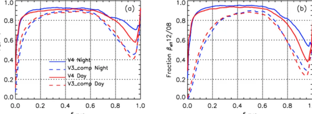
3.3.1 Fraction of samples in sensitivity range
Figure 6a and b show fractions of samples for which βeff12/10 and βeff12/08 are larger than their respective
theo-retical lower ranges, which were derived for De=120 µm
using the V4 SCO LUT, and in practice are close to 1. For both βeff12/10 and βeff12/08, V4 retrievals are
possi-ble more than 80 % of the time for εeff,12between 0.05 and
0.80 (or about 0.1–3.2 in terms of τvis). In contrast, the εeff,12
80 % range in V3_comp was only 0.15–0.7 for the 12/10 pair and only 0.25–0.7 for the 12/08 pair. As εeff,12increases
from 0.8 to 0.95 (τvis∼6), which corresponds to clouds that
are opaque to CALIOP (see Fig. 2), the βeff12/ k indices
de-crease and approach the sensitivity limit, and the fraction of possible retrievals in opaque clouds decreases. This fraction is notably increased in V4 and is larger at night than for day-time data, reflecting the impact of the cloud radiative tem-perature corrections introduced in V4. As in V3, this frac-tion remains lower for the 12/08 pair. One hypothesis is that cloud heterogeneities in dense clouds could induce a larger low bias in the 12/08 pair than in the 12/10 pair (Fauchez et al., 2015). The V4 nighttime retrieval rate is larger than 70 % up to εeff,12=0.95 for the 12/10 pair and up to εeff,12=0.9
Figure 3. IIR inter-channel (a) 1εeff12–10 and (b) 1εeff12–08 effective emissivity differences vs. effective emissivity at 12.05 µm in single-layered ice clouds over oceans between 60◦S and 60◦N in January 2008 in V4 (solid lines) and in V3_comp (dashed lines). The blue and red curves are median values for nighttime and daytime data, respectively. The shaded gray areas are between the V4 nighttime 25th and 75th percentiles.
Figure 4. (a) Nighttime and (b) daytime comparisons of V3 and V4 IIR cloud optical depth (τvis) in single-layered ice clouds over oceans between 60◦S and 60◦N in January 2008. The small embedded plots show details for τvisbetween 0 and 1.
3.3.2 Changes in effective diameters
Because the changes in the microphysical indices are larger for the 12/08 pair than for the 12/10 pair, we now assess the changes in the respective diameters, De12/08 and De12/10.
For meaningful comparisons, the exercise is carried out only for clouds for which both βeff12/10 and βeff12/08 are found
above the lower sensitivity limit, both in V3 and in V4. The changes in De12/10 and in De12/08 are illustrated in
Fig. 7a and b, respectively. The solid lines represent median De12/ k derived from V4 βeff12/ k and the V4 SCO LUT.
The dashed lines represent median De12/ k derived from
V3_comp βeff12/ k and the same V4 SCO LUT, so the
dif-ferences between the solid and the dashed lines are due only to the different microphysical indices. As a result of changes of different amplitude for De12/10 and De12/08, the
consis-tency between these two diameters is drastically improved in V4 at εeff,12 smaller than 0.5. Similar conclusions would be
drawn using the V4 CO8 model.
For a complete analysis of the differences between the V3_comp and V4 diameters, the dashed–dotted lines show De12/ k derived using V3_comp and the V3 solid column
LUT (Part I), so the differences between the dashed–dotted lines and the dashed lines are due only to the different LUTs. The changes resulting from the LUTs and from the micro-physical indices have an opposite effect, regardless of the specific V3 and V4 LUTs chosen for the analysis. As a result, De12/10 is overall not changed significantly in V4
(solid lines) compared to V3_comp (dashed–dotted lines). In contrast, De12/08 is smaller in V4 by up to 15 µm at
εeff,12<0.2, because the improved (and increased) βeff12/08
has the largest impact, and conversely V4 De12/08 is larger
by up to 10 µm at εeff,12between 0.2 and 0.9.
3.4 V4 microphysical retrievals
We showed in Sect. 3.3 that the fraction of samples with possible microphysical retrievals is significantly increased in V4 (Fig. 6), and that the consistency between the De12/10
and De12/08 diameters is drastically improved (Fig. 7). The
significant disagreement between De12/10 and De12/08
in V3_comp was due to biases of different amplitude in βeff12/10 and βeff12/08, and could not be explained by the
Figure 5. (a) βeff12/10 and (b) βeff12/08 microphysical indices vs. effective emissivity at 12.05 µm in single-layered ice clouds over oceans between 60◦S and 60◦N in January 2008 in V4 (solid lines) and in V3_comp (dashed lines). The blue and red curves are the median values for nighttime (blue) and daytime (red), and the shaded gray areas are between the V4 nighttime 25th and 75th percentiles. The blue (night) and red (day) thin dashed–dotted lines are the V4 random absolute uncertainty estimates with the vertical axis on the right-hand side of each panel.
Figure 6. Fraction of (a) βeff12/10 and (b) βeff12/08 values above the effective diameter retrieval sensitivity limit vs. effective emissivity at 12.05 µm in single-layered ice clouds over oceans between 60◦S and 60◦N in January 2008 in V4 (solid lines) and in V3_comp (dashed lines) during night (blue) and day (red).
V3 and in V4, De is retrieved using the ice habit model
found in best agreement with IIR in terms of relationship be-tween βeff12/10 and βeff12/08. Because the accuracy of IIR
βeff12/ k is improved in V4, the residual discrepancies with
respect to the ice habit models are expected to be a genuine piece of information about ice crystal shape. This requires both βeff12/ k to be found within the sensitivity range, which
hereafter will be called “confident” retrievals. Because the population of clouds meeting this requirement is larger in V4 than in V3 and covers a larger range of optical depths, the results in this section will be shown for V4 only.
Theoretically, confident retrievals should be found when De is smaller than 120 µm and βeff12/ k should tend to the
upper sensitivity limit for De>120 µm. In practice,
uncer-tainties in βeff12/ k can trigger non-confident retrievals even
if De is truly smaller than the sensitivity limit, and this is
more likely to occur when De is close to this limit.
Requir-ing both βeff12/ k to be in the expected range of values is
meant to reinforce the confidence in the retrievals, but doing so implies no systematic bias between both pairs of channels. This is not exactly true for opaque clouds with εeff,12> ∼0.8
(Fig. 6), and consequently the fraction of confident retrievals in opaque clouds is often constrained by the 12/08 pair. Fur-thermore, the fraction of confident retrievals at large emissiv-ities is larger at night.
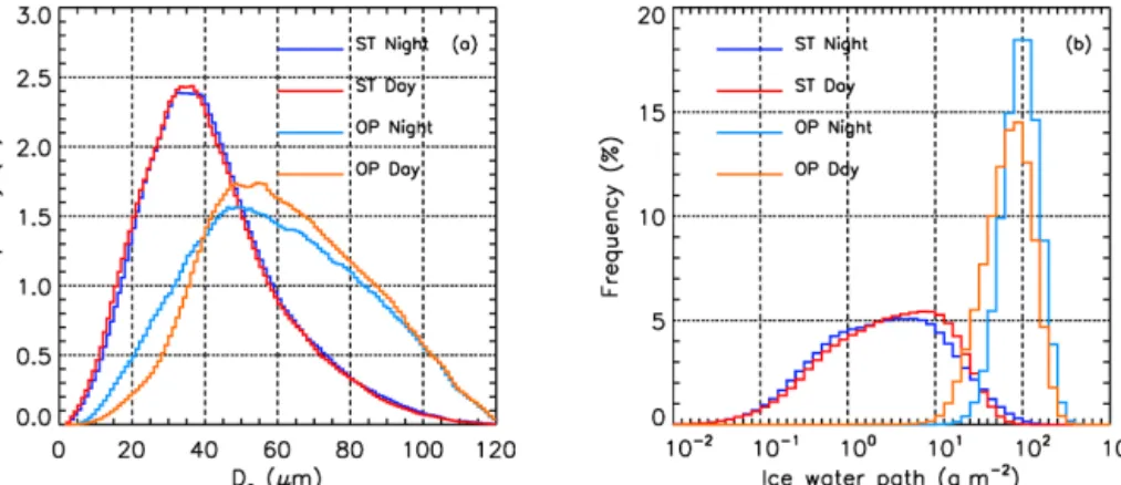
3.4.1 Effective diameter and ice water path
The histograms of confident Deand ice water path retrievals
(IWP) are shown in Fig. 8a and b, respectively, for ST and opaque clouds, and statistics are reported in Table 4. The IWP histograms are computed in logarithmic scale between 0.01 and 1000 g m−2, with log10(IWP) bins equal to 0.1. The
random uncertainty in De, noted 1De, is computed based on
the LUT selected for the retrieval and the estimated random uncertainty in the βeff12/ k indices. Median 1De/Devalues
reported in Table 4 are between 34 % and 49 %. The uncer-tainty in IWP is in large part driven by the unceruncer-tainty in De.
The ST clouds are optically thin, with median IIR τvis of
only 0.2–0.26. Their nighttime (navy blue) and daytime (red) Dedistributions are nearly identical, with median De=38–
39 µm and a peak around De=35 µm. This peak compares
Figure 7. (a) Median De12/10 and (b) median De12/08 vs. effective emissivity at 12.05 µm for the cloud population used in Fig. 6, except that both βeff12/10 and βeff12/08 are in the range of possible retrievals, both in V3_comp and in V4. Solid line: V4 with SCO LUT; dashed lines: V3_comp with V4 SCO LUT; dashed–dotted line: V3_comp with V3 solid column LUT. Blue: night; red: day.
Figure 8. Histograms of V4 confident retrievals of (a) Deand (b) ice water path in single-layered semi-transparent (ST; night: navy blue; day: red) and opaque (OP; night: light blue; day: orange) ice clouds between 60◦S and 60◦N over oceans in January 2008.
Table 4. Statistics associated with V4 effective diameter (De) and ice water path (IWP) retrievals in single-layered ice clouds between 60◦S and 60◦N over oceans in January 2008 (see Fig. 8).
Ice clouds Semi-transparent Opaque Night Day Night Day Number of pixels 167 152 201 534 98388 138 193 Median εeff,12 0.11 0.13 0.95 0.86
Median IIR τvis 0.22 0.26 5.6 3.8
Median De(µm) 39 38 58.5 61
Median 1De(µm) 18 17 28 21
Median 1De/De 0.49 0.46 0.48 0.34
Median IWP (g m−2) 2.7 3.2 97 71 Median 1IWP (g m−2) 1.3 1.4 50 24 Median 1IWP / IWP 0.54 0.49 0.50 0.35
for single-layered ice clouds with no detectable precipitation as retrieved using the combined CloudSat-CALIPSO 2C-ICE product. IWP (Fig. 8b) is found between 0.03 and 100 g m−2 in ST clouds, with the slightly larger daytime values being explained by the cloud selection and the slightly larger opti-cal depths in the daytime dataset (Table 4). The medium
val-ues are around 3 g m−2, with peaks in the distributions at 3 and 8 g m−2for nighttime and daytime data, respectively, and the median relative uncertainty is 50 %. As noted by Berry and Mace (2014), the CloudSat radar is typically insensi-tive to these thin layers, so microphysical retrievals in com-bined CloudSat-CALIPSO products such as 2C-ICE rely on parameterization of the radar reflectivity (Deng et al., 2015) rather than on actual observations. Combining CALIOP and IIR observations appears to be a suitable alternative approach to characterize these thin layers.
The estimated cloud radiative temperature (Tr) is at an
equivalent altitude located between the CALIOP cloud base and cloud top (Part I). While in the case of ST clouds, IIR De
is a layer average diameter, IIR Dein opaque clouds is mostly
representative of the portion of the cloud seen by CALIOP before the signal is totally attenuated. These opaque clouds have median εeff,12 equal to 0.95 at night but only 0.86 for
daytime data, with median IIR τvis equal to 5.6 and 3.8,
re-spectively. Median Dein opaque clouds is around 60 µm and
the distributions peak at 50 µm. It is larger than in ST clouds, which is consistent with retrievals based on AIRS thermal infrared data (Guignard et al., 2012; Kahn et al., 2018). The different nighttime and daytime Deand IWP distributions in
opaque clouds are explained by the different ranges of optical depth and the different amplitudes of the radiative tempera-ture correction (Figs. 2 and 4). In opaque clouds, the retrieved IWP lies between 10 and only 300 g m−2. The upper limit is due to the fact that Decannot be larger than 120 µm and
be-cause cloud optical depths inferred from IIR effective emis-sivities saturate and are typically smaller than 15 (Fig. 4). 3.4.2 Ice habit model selection
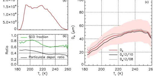
Recall that De is retrieved using the habit model (SCO or
CO8) that agrees the best with IIR in terms of the relation-ship between βeff12/10 and βeff12/08. As seen in Fig. 9, the
SCO habit model is selected in 80 % of the ST clouds of Tr<205 K. This fraction steadily decreases down to 60 % as
Trincreases up to 230 K (Fig. 9b) and remains stable above
230 K. This result is qualitatively consistent with previous findings using V3 (Garnier et al., 2015), and, as was dis-cussed in this paper, both the IIR model selection and the mean CALIOP integrated particulate depolarization ratio (in black in Fig. 9b) indicate changes of crystal habit with tem-perature. In opaque clouds (Fig. 10), both the IIR model se-lection and the CALIOP depolarization ratio between 200 and 230 K are less temperature dependent than in ST clouds. The difference between mean De12/10 and mean De12/08
in black and gray in Figs. 9c and 10c is a measure of the residual mismatch between IIR observations and the selected model. We see two temperature regimes, that is, below and above 225 K, with a better agreement between IIR and the LUTs at the warmer temperatures. This suggests that the V4 models are better suited for warmer clouds and that they do not perfectly reproduce the infrared spectral signatures of colder clouds composed of small crystals. It is acknowl-edged that the highly variable ice particle shapes found in ice clouds (Lawson et al., 2019 and references therein) are likely not fully reproduced through the two models chosen for the V4 algorithm. It is further noted that the Clouds and the Earth’s Radiant Energy System (CERES) science team is planning to use a two-habit model for retrievals in the visible–near-infrared spectral domain (Liu et al., 2014; Loeb et al., 2018). This model would be a mixture of two habits (single column and an ensemble of aggregates) whose mix-ing ratio would vary with ice crystal maximum dimension, with single columns prevailing for the smaller dimensions. Interestingly, our findings appear to be consistent with this approach.
In both thin ST clouds (Fig. 9c) and opaque clouds (Fig. 10c), Deincreases with cloud radiative temperature
un-til it reaches a maximum value around 250 K in ST clouds and 230 K in opaque clouds. Kahn et al. (2018) found that for clouds of emissivity smaller than 0.98 (or τvis smaller
than about 8), De is maximum and around 50 µm at 230 K,
which is consistent with our findings, keeping in mind that clouds with emissivity smaller than 0.98 are found in both our ST and opaque clouds. The increase of cloud average
Dewith cloud radiative temperature in ST clouds (Fig. 9c) is
in general agreement with numerous previous findings (e.g., Hong and Liu, 2015). The decrease of Debetween Tr=250
and 260 K for ST clouds is possibly due to an increasing frac-tion of small liquid droplets in these prevailingly ice layers, which would be consistent with the fact that the CALIOP in-tegrated particulate depolarization ratio decreases from 0.37 to 0.30 (Fig. 9b). Similar comments apply for opaque clouds for Tr between 230 and 260 K. Using combined POLDER
(POLarization and Directionality of the Earth’s Reflectances) and MODIS data, Van Diedenhoven et al. (2020) found that Deat the top of thick clouds of optical depth larger than 5
is maximum at cloud top temperature equal to 250 K, rather than Tr=230 K for opaque clouds. This discrepancy might
be partly explained if the cloud radiative altitude is higher in the cloud than the cloud top derived from the visible ob-servations, which could also explain that De shown in van
Diedenhoven et al. (2020) is larger than that in this study. 3.4.3 Retrievals using parameterizations from in situ
formulation
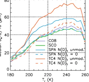
The IIR algorithm takes advantage of the relationship be-tween βeff12/10 and βeff12/08 to identify the ice habit model
that best matches the observations and thereby provide in-formation about both ice crystal shape and effective diam-eter. Another approach would be to use only βeff12/10 and
prescribed LUTs. This approach was adopted by Mitchell et al. (2018), who derived four sets of LUTs using extensive in situ measurements rather than pure modeling. In Part I, we compared these four sets of βeff12/10–De relationships
with the relationships derived from the V4 SCO and CO8 models. The four sets of De derived from βeff12/10 using
this independent approach are reported in the IIR product for the user’s convenience. Figure 11 compares Decomputed by
the analytic function derived by Mitchell et al. (2018) with De12/10 from the CO8 and the SCO models. Relationships
derived from the Small Particles in Cirrus Science and Op-erations Plan (SPARTICUS) (blue) and the Tropical Compo-sition, Cloud, and Climate Coupling (TC4) (red) field cam-paign were computed in two ways: by setting the first bin of the measured particle size distribution (PSD) (D<15 µm) to 0 (i.e., N (D)1=0, dashed lines) and without modifying
the distribution (i.e., N (D)1unmodified, solid lines). As
dis-cussed in Part I, the differences between the six sets of re-trievals illustrate the possible impacts of the LUTs and of the PSDs. Because the presence of small particles in the un-modified PSD causes βeff12/10 to increase faster than De,
assuming N (D)1=0 yields smaller values of Defor a given
βeff12/10 than when N (D)1 is not modified. Even though
this was not the original intent, comparing median Dewith or
without setting N (D)1to 0 also illustrates the impact of
pos-sible vertical inhomogeneities of De within the cloud layer
(Zhang et al., 2010). Nevertheless, the overall impact of ver-tical variations on βeff12/10 also depends on the in-cloud IIR
Figure 9. IIR V4 confident retrievals vs. radiative temperature in semi-transparent ice clouds over oceans between 60◦S and 60◦N in January 2008. (a) Pixel count; (b) fraction of retrievals using the SCO model (green) and mean CALIOP integrated particulate depolarization ratio (black); (c) mean De(red) ± mean absolute deviation (shaded area), mean De12/10 (black) and mean De12/08 (gray).
Figure 10. Same as Fig. 9 but for opaque clouds.
weighting function, which is related to the cloud extinction profile (Part I). In Mitchell et al. (2020), the mean De
cal-culated from the SPARTICUS unmodified βeff12/10–De
re-lationship (applied at midlatitudes) and the TC4 N (D)1=0
βeff12/10–Derelationship (applied in the tropics) was
com-pared against the in situ climatology of mean volume radius, Rv, reported in Krämer et al. (2020) after converting Deto
Rv. The retrieved Rv tended to be no more than ∼ 20 %
smaller than the in situ Rvfor temperatures between 208 and
233 K.
3.5 Comparisons with MODIS
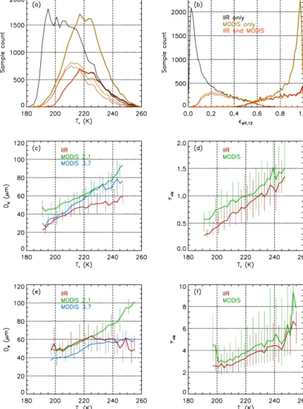
Figure 12 compares IIR confident retrievals and co-located MODIS/Aqua Collection 6 daytime retrievals from the visible–2.1 µm and visible–3.7 µm pairs of channels (Plat-nick et al., 2017, and references therein) in single-layered clouds classified as high-confidence ROIs by CALIOP and as
ice clouds by MODIS. MODIS τvisand Deat 1 km resolution
are from the MYD06 product and co-location with CALIPSO is from the AERIS/Cloud-Aerosol-Water-Radiation Interac-tions (AERIS/ICARE) CALTRACK product. Analyses are over oceans between 30◦S and 30◦N in January 2008 sepa-rately for CALIPSO ST and opaque clouds. Figure 12a and b show the population of clouds with IIR retrievals (black), with MODIS retrievals at both 2.1 and 3.7 µm (brown), and with both IIR and MODIS retrievals (orange) for which com-parisons in Fig. 12c–f are shown. Figure 12a and b charac-terize these cloud populations as a function of IIR Tr and
IIR εeff,12, respectively. For ST clouds (thin lines), the IIR–
MODIS comparisons are constrained by the availability of MODIS retrievals, and the compared ST clouds have εeff,12
typically larger than 0.2 (Fig. 12b). In contrast, comparisons in opaque clouds (thick lines) are limited by the availabil-ity of IIR retrievals. Figure 12c and e show median Defrom
Figure 11. Median De12/10 from the V4 CO8 (purple) and SCO (green) models, and from analytical functions derived by Mitchell et al. (2018) during the SPARTICUS (blue) and TC4 (red) field ex-periments using N (D)1unmodified (solid) or N (D)1=0 (dashed). This is the same dataset as the one in Fig. 9.
for ST (Fig. 12c) and opaque (Fig. 12e) clouds. The vertical lines are between the 25th and 75th percentiles. Similarly, Fig. 12d and f show the corresponding τvisvalues. Only one
MODIS τvis is shown because the retrievals from both pairs
of MODIS channels are nearly identical.
For ST clouds, MODIS 2.1 Deis larger than IIR by 15 µm
on average. IIR and MODIS 3.7 Deare in good agreement
for Tr<205 K, where Deis <40 µm and IIR τvisis <0.5, and
they progressively depart from each other as Trincreases and
MODIS 3.7 increases and approaches MODIS 2.1. MODIS τvis is larger than IIR by 0.3 to 0.2. This small but
sys-tematic bias is not seen when comparing CALIOP and IIR (not shown). The MODIS 2.1 De–Trrelationships are
sim-ilar for ST and opaque clouds, which is not the case for MODIS 3.7 and IIR. For opaque clouds, IIR De is larger
than in ST clouds and is in good agreement with MODIS 2.1 at Tr<225 K. MODIS 3.7 De exhibits a similar increase
with temperature as seen with the two other datasets, but it is shifted by −10 µm. At Tr>225 K, MODIS De2.1 continues
to increase up to 100 µm at 255 K, whereas IIR remains stable around 60 µm and MODIS 3.7 increases slowly to approach the same plateau as IIR around 60 µm. As seen in Fig. 12f, both MODIS and IIR indicate moderate optical depths in these opaque clouds where comparisons are possible, with median values ranging between 2.5 and 6 at Tr<250 K, IIR
being smaller than MODIS by about 0.4.
Kahn et al. (2015) found that MODIS 2.1 Deis typically
larger than AIRS De by 10–20 µm, and that MODIS 3.7 is
in better agreement with AIRS on average. These results, which were for clouds of optical depth between 0.5 and 2 over oceans, are consistent with our findings for ST clouds. The MODIS and IIR techniques exhibit different non-linear
sensitivities to particle size, so vertical inhomogeneities of the effective diameter can yield three different retrieved De
values (Zhang et al., 2010). This could explain that IIR De
is found in better agreement with MODIS 3.7 in ST clouds while MODIS 2.1 is clearly larger (Zhang et al., 2010). At Tr>220 K, IIR De is around 50–60 µm and smaller than
both MODIS 2.1 and 3.7. We note that the agreement with MODIS would be improved using the parameterized func-tions derived from the unmodified in situ PSDs that were presented in Sect. 3.4.3 but that the modified PSDs would yield similar results. For clouds of moderate optical depth as found in our population of opaque clouds, MODIS 3.7 is very sensitive to cloud top while MODIS 2.1 senses deeper into the cloud (Zhang et al., 2010; Platnick, 2000), and the smaller MODIS 3.7 Deas observed in Fig. 12e suggests that
the effective diameter is smaller at cloud top than deeper into the cloud. IIR Demight be larger than MODIS 3.7 and
in better agreement with MODIS 2.1 for opaque clouds at Tr<220 K because the IIR weighting function is deeper in the
cloud than at 3.7 µm, which is agreement with simulations by Zhang et al. (2010). In conclusion, distinct sensitivity to possible cloud vertical and horizontal (Fauchez et al., 2018) inhomogeneity likely contributes to the observed differences.
4 V4 retrievals in liquid water clouds
The only difference between effective emissivity V4 re-trievals in liquid and ice clouds is that Tris taken as the
tem-perature at the CALIOP centroid altitude (Tc) in the case of
liquid water clouds, whereas this initial temperature estimate is further corrected in the case of ice clouds. It is recalled that Deof liquid droplets are retrieved using the water LUTs
(Part I) and that liquid water path is derived from De and
εeff,12(Eq. 12 in Part I).
Following a similar approach as for ice clouds, the results are shown for scenes over oceans between 60◦S and 60◦N that contain a single cloud layer classified as high-confidence water by the CALIOP phase algorithm. Because liquid water clouds are statistically warmer than ice clouds, the radiative contrast is typically smaller than for ice clouds. Because un-certainties are inversely proportional to this radiative contrast (Part I), they increase very rapidly when the radiative tem-perature contrast, that is the difference between the clear air TOA background brightness temperature and the TOA black-body brightness temperature, is smaller than 10 K. In order to prevent very large uncertainties associated with very small radiative contrast, the results are presented for clouds in the free troposphere with centroid altitude above 4 km. For this cloud population, the radiative temperature contrast is larger than 10 K, and it increases on average from 15 K at 4 km to 50 K at 10 km where the highest water clouds are found (not shown). Most of these sampled liquid clouds are composed of supercooled droplets.
Figure 12. IIR and MODIS comparisons over oceans between 30◦S and 30◦N in January 2008 for single-layered high-confidence ROI clouds with MODIS ice phase. Distributions of (a) IIR radiative temperature and (b) IIR effective emissivity at 12.05 µm in ST (thin lines) and opaque (thick lines) clouds where IIR has confident retrievals (black), MODIS has successful retrievals at 2.1 and 3.7 µm (brown), and both IIR and MODIS retrievals are successful and can be compared (orange). Median De vs. Trfrom IIR (red), MODIS 2.1 (green) and MODIS 3.7 (blue) in ST (c) and opaque (e) clouds; median τvisfrom IIR (red) and MODIS (green) in ST (d) and opaque (f) clouds. The vertical bars in panels (c–f) are between the 25th and 75th percentiles.
Our results are presented in Sect. 4.1 to 4.3 and compar-isons with MODIS are shown in Sect. 4.4.
4.1 Effective emissivity in channel 12.05
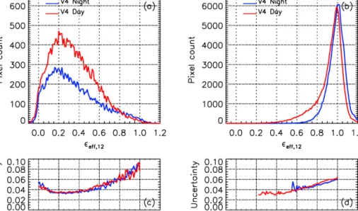
Figure 13a and b show the distributions of V4 εeff,12 in ST
and opaque liquid water clouds, respectively, for the month of January 2008 between 60◦S and 60◦N over ocean, for
clouds with centroid altitude >4 km. Figure 13c and d show the respective median random uncertainties, which are about twice as large as the uncertainties in ice clouds (Fig. 2c and d) because of the smaller radiative contrast. Only 17 % of these clouds are ST (Fig. 13a and c). Unlike in ST ice clouds, the distributions peak at εeff,12∼0.2, and non-physical negative
emissivity values are found in only 2 % of the pixels. The
εeff,12 distributions in opaque clouds peak at 1.02 at night
and at 0.99 for daytime data, with an estimated uncertainty of ±0.06. The spread around these peaks is larger than for ice clouds, which is explained by the larger uncertainties and specifically to a larger sensitivity to a wrong estimate of Tr.
Thus, the nighttime and daytime fractions of samples with εeff,12>1, for which no microphysical retrievals are possible,
are 45 % and 27 %, respectively. The daytime distributions in opaque clouds exhibit a tail down to εeff,12∼0.4, while
at night, the lowest εeff,12 is ∼ 0.65, which is very similar
to what was observed for opaque ice clouds (Fig. 2b). This similarity suggests that emissivity retrievals in ice and liquid water clouds are consistent, notwithstanding the unavoidable larger uncertainties in the latter ones.
Figure 13. V4 effective emissivity distribution at 12.05 µm in (a) ST and (b) opaque single-layered liquid water clouds of centroid altitude >4 km over oceans between 60◦S and 60◦N in January 2008 for nighttime (blue) and daytime (red) data. Panels (c) and (d) are the V4 median random uncertainties corresponding to panels (a) and (b), respectively.
4.2 Inter-channel effective emissivity differences The variations with εeff,12of the V4 1εeff12−k inter-channel
effective emissivity differences for the 12–10 and 12–08 pairs are shown in Fig. 14a and b, respectively. The night-time (blue) and daynight-time (red) curves are median values, and the shaded gray areas are between the V4 nighttime 25th and 75th percentiles. As for ice clouds, both 1εeff12 − k tend
nicely to 0 at εeff,12∼0, due to the improved computed
back-ground radiances demonstrated previously, which has a ben-eficial effect on retrievals in any ST layer. Both 1εeff12 − k
have a second minimum at εeff,12∼1, as expected, and this
minimum is found slightly larger than 0. Both 1εeff12 − k
values and therefore both βeff12/ k values are notably larger
than for ice clouds (see Fig. 3), reflecting the presence of smaller particles in the liquid water distributions (Giraud et al., 2001; Mitchell and d’Entremont, 2012). As shown by Avery et al. (2020), the IIR microphysical indices are un-ambiguously larger in clouds classified as liquid water by the CALIOP phase algorithm than in clouds classified as ice.
4.3 Microphysical retrievals
4.3.1 Effective diameter and liquid water path
As previously, retrievals are deemed confident when both βeff12/ k are found within the sensitivity range, which
cor-responds to De=60 µm for liquid clouds. The fraction of
confident retrievals is found similar in liquid water clouds of centroid altitude >4 km and in ice clouds. Following the same presentation as for ice clouds, the histograms of confi-dent Deand liquid water path (LWP) retrievals are shown in
Table 5. Statistics associated to V4 effective diameter (De) and LWP retrievals in single-layered liquid water clouds of centroid al-titude >4 km between 60◦S and 60◦N over oceans in January 2008 (see Fig. 15).
Ice clouds Semi-transparent Opaque Night Day Night Day Number of pixels 11 562 18 887 36 998 54 169 Median εeff,12 0.33 0.34 0.94 0.89
Median IIR τvis 0.88 0.87 5.23 4.15
Median De(µm) 13 13.5 18 18.5 Median 1De(µm) 5.6 5.7 9 8 Median 1De/De 0.46 0.45 0.52 0.42 Median LWP (g m−2) 3.3 3.4 31 25 Median 1LWP (g m−2) 1.1 1.2 15 10 Median 1LWP / LWP 0.35 0.35 0.48 0.39
Fig. 15a and b, respectively, for ST and opaque clouds, and statistics are reported in Table 5.
Note that the IIR retrievals shown in Fig. 15 are for a pop-ulation of optically thin water clouds: median τvisis only 0.9
in ST clouds and between 4 and 5 in opaque clouds. Both in ST and in opaque clouds, the nighttime and daytime De
histograms are similar. In ST clouds, median De is 13 µm
and median liquid water path is 3.4 g m−2with a median ran-dom uncertainty of 1.2 g m−2. In opaque clouds, median De
is 18 µm and median liquid water path is 25–31 g m−2with a median random uncertainty of 10–15 g m−2. The maximum retrieved LWP is about 100 g m−2, consistent with the in-frared saturation range of 40–60 g m−2 reported by Marke et al. (2016) who combined microwave and infrared ground-based observations to improve LWP and De retrievals in
Figure 14. V4 IIR inter-channel (a) 1εeff12–10 and (b) 1εeff12–08 effective emissivity differences vs. effective emissivity at 12.05 µm in single-layered liquid water clouds of centroid altitude >4 km over oceans between 60◦S and 60◦N in January 2008. The blue and red curves are median values for nighttime and daytime data, respectively. The shaded gray areas are between the V4 nighttime 25th and 75th percentiles.
Figure 15. Histograms of V4 confident retrievals of (a) Deand (b) liquid water path in single-layered semi-transparent (ST; night: navy blue; day: red) and opaque (OP; night: light blue; day: orange) liquid water clouds of centroid altitude >4 km between 60◦S and 60◦N over oceans in January 2008.
“thin” clouds that they defined as LWP <100 g m−2. The au-thors report Debetween 10 and 14 µm in “thin” clouds of top
altitude < ∼ 1 km, which agrees well with the peaks of our distributions.
4.3.2 Analyses vs. radiative temperature
IIR retrievals in ST liquid water clouds are shown in Fig. 16 as a function of Tr, highlighting that most of these liquid
clouds of centroid altitude >4 km are supercooled, with Tr
ranging between 235 and 280 K (Fig. 16a). Mean IIR De
(Fig. 16b, red) increases steadily from 11 µm at 242 K to 18 µm at 270 K, while mean CALIOP particulate depolar-ization ratio (Fig. 16c) is constant and around 0.1. These thin clouds are likely radiation driven, and the increase of layer average Dewith layer radiative temperature could
indi-cate growth through vapor deposition. In addition, there is an increasing probability for supercooled droplets to freeze as temperature decreases. As Trdecreases from 242 to 235 K,
the number of samples drops quickly, De increases up to
24 µm, and CALIOP depolarization ratio increases very
sig-nificantly, confirming a rapid transition to ice phase. At Tr >270 K, De continues to increase slightly up to 20 µm,
while CALIOP integrated particulate depolarization ratio de-creases. As seen in Fig. 16b, De12/10 and De12/08 are in
fair agreement. The mean De12/10 − De12/08 difference
increases from −2 µm at 275 K to +3 µm at 245 K. This slight temperature-dependent discrepancy between the IIR observations and the water LUT could be explained by the fact that the complex refractive index is temperature de-pendent, as reported by Zasetsky et al. (2005) and Wag-ner et al. (2005), the complex refractive index of super-cooled water being intermediate between warm water and ice (Rowe et al., 2013). Further investigations will be carried out to establish whether the residual discrepancy between De12/10 and De12/08 would be reduced by using a new set
of temperature-dependent indices, following the approach in Rowe et al. (2013). Nevertheless, these simple observations give confidence in the new V4 IIR Deretrievals in ST liquid