HAL Id: hal-00296238
https://hal.archives-ouvertes.fr/hal-00296238
Submitted on 24 May 2007
HAL is a multi-disciplinary open access
archive for the deposit and dissemination of
sci-entific research documents, whether they are
pub-lished or not. The documents may come from
teaching and research institutions in France or
abroad, or from public or private research centers.
L’archive ouverte pluridisciplinaire HAL, est
destinée au dépôt et à la diffusion de documents
scientifiques de niveau recherche, publiés ou non,
émanant des établissements d’enseignement et de
recherche français ou étrangers, des laboratoires
publics ou privés.
deposition: tropospheric model simulations with
ECHAM5/MESSy1
H. Tost, P. Jöckel, A. Kerkweg, A. Pozzer, R. Sander, J. Lelieveld
To cite this version:
H. Tost, P. Jöckel, A. Kerkweg, A. Pozzer, R. Sander, et al.. Global cloud and precipitation chemistry
and wet deposition: tropospheric model simulations with ECHAM5/MESSy1. Atmospheric Chemistry
and Physics, European Geosciences Union, 2007, 7 (10), pp.2733-2757. �hal-00296238�
www.atmos-chem-phys.net/7/2733/2007/ © Author(s) 2007. This work is licensed under a Creative Commons License.
Chemistry
and Physics
Global cloud and precipitation chemistry and wet deposition:
tropospheric model simulations with ECHAM5/MESSy1
H. Tost, P. J¨ockel, A. Kerkweg, A. Pozzer, R. Sander, and J. Lelieveld
Atmospheric Chemistry Department, Max Planck Institute for Chemistry, P.O. Box 3060, 55020 Mainz, Germany Received: 23 November 2006 – Published in Atmos. Chem. Phys. Discuss.: 18 January 2007
Revised: 4 May 2007 – Accepted: 16 May 2007 – Published: 24 May 2007
Abstract. The representation of cloud and precipitation chemistry and subsequent wet deposition of trace con-stituents in global atmospheric chemistry models is asso-ciated with large uncertainties. To improve the simulated trace gas distributions we apply the new submodel SCAV, which includes detailed cloud and precipitation chemistry and present results of the atmospheric chemistry general cir-culation model ECHAM5/MESSy1. A good agreement with observed wet deposition fluxes for species causing acid rain is obtained. The new scheme enables prognostic calcula-tions of the pH of clouds and precipitation, and these re-sults are also in accordance with observations. We address the influence of detailed cloud and precipitation chemistry on trace constituents based on sensitivity simulations. The results confirm previous results from regional scale and box models, and we extend the analysis to the role of aqueous phase chemistry on the global scale. Some species are di-rectly affected through multiphase removal processes, and many also indirectly through changes in oxidant concentra-tions, which in turn have an impact on the species lifetime. While the overall effect on tropospheric ozone is relatively small (<10%), regional effects on O3can reach ≈20%, and
several important compounds (e.g., H2O2, HCHO) are
sub-stantially depleted by clouds and precipitation.
1 Introduction
Scavenging and subsequent wet deposition represent impor-tant removal processes for many trace constituents in the troposphere. They are crucial for cleansing the troposphere from aerosol particles and soluble gases and indirectly also for many less soluble species. Furthermore, multiphase chemistry can have a major impact on tropospheric
compo-Correspondence to: H. Tost
sition (Ravishankara, 1997). However, the representation of wet deposition and cloud chemistry differs widely in global models, resulting in large uncertainties (Rasch et al., 2000). These uncertainties are to a large extent associated with the coarse descriptions of cloud and precipitation processes, and also with the representation of scavenging and aqueous phase chemistry (Zhang et al., 2006). Even though Levine and Schwartz (1982) and Schwartz (1986) have shown more than two decades ago that for most gases uptake according to Henry’s equilibrium alone does not represent atmospheric conditions, this approximation is still commonly used in scavenging parameterisations, in particular in global mod-els. Alternatively, fixed scavenging coefficients are applied, implicitly assuming that the process only varies as a function of the precipitation flux. The treatment of chemical reactions of dissolved gases in clouds and precipitation has largely fo-cused on sulphur species (e.g. Berglen et al., 2004).
A model intercomparison of cloud chemical parcel mod-els focusing mainly on the oxidation of SO2 in the
aque-ous phase (including the basic aqueaque-ous phase transfer and chemical reactions) has shown that large uncertainties arise from different parameterisations (Kreidenweis et al., 2003). More detailed cloud chemistry schemes have been applied in smaller scale models (box models, cloud parcel mod-els, single column models), e.g. by Chameides and Davis (1982); Jacob (1986); Lelieveld and Crutzen (1991); Bott and Carmichael (1993); Monod and Carlier (1999); Fahey and Pandis (2001); von Glasow et al. (2002); Ervens et al. (2003); Leriche et al. (2003); Barth et al. (2003) and references therein; Kreidenweis et al. (2003) and references therein, and detailed information about the processes involved has been gained. However, from these results it is difficult to estimate the large-scale effects of multiphase chemistry. Lelieveld and Crutzen (1991) have derived the global tropospheric impact by applying their chemical box-model in combination with a global cloud data set. The application of the model of Liang and Jacob (1997) in the regional model of Jacob et al.
(1993) leads to the conclusion of a minor impact of multi-phase chemistry on the regional scale, although this was only valid for the simulated period and domain addressed, and the extrapolation to the global scale is not straightforward.
Fahey and Pandis (2003) have increased the amount of de-tail and the model complexity, and calculated droplet size resolved cloud chemistry in a 3D regional transport model. Yet, this model setup is quite complex and therefore it has not been applied in an atmospheric chemistry general circu-lation model (AC-GCM). Global models including cloud and precipitation chemistry often lack comprehensiveness to sim-ulate the interconnected effects in the gas and liquid phase. For example, Stier et al. (2005) calculated in-cloud SO2
ox-idation, but used prescribed distributions for the oxidants. Since some of these models aim at the investigation of the global sulphur cycle (e.g. Feichter et al., 1996; Rostayn and Lohmann, 2002; Dentener et al., 2006; Berglen et al., 2004), this might be appropriate, though it also introduces large un-certainties. Crutzen and Lawrence (2000) determined the ef-fects of trace gas scavenging in a 3D global model, however, did not assess multiphase chemistry in clouds and precip-itation. Global model studies explicitly considering aque-ous phase chemistry may exist (e.g. Dentener, 1993), though not reported in the peer reviewed literature. Dentener and Crutzen (1993, 1994) applied several heterogeneous reac-tions including NH3 chemistry and their influence on gas
phase composition. Roelofs and Lelieveld (1995) introduced additional aqueous phase reactions including e.g., HCHO and HCOOH in their model to assess multiphase chemistry, although non-methane-hydrocarbon (NMHC) chemistry was neglected and both the gas and aqueous phase reaction mech-anisms applied are not easily expandable.
In the present study the scavenging and subsequent wet deposition of trace species in the ECHAM5/MESSy1 model is presented, and the influence of more detailed cloud and precipitation chemistry on the tropospheric composition is investigated with the recent submodel SCAV (Tost et al., 2006a). Following a short model description in Sect. 2, the simulation setup is outlined in Sect. 3. The results, presented in Sect. 4, distinguish three aspects: the evaluation of the wet deposition fluxes (4.1), the analysis of global pH values in clouds and precipitation (4.2) and the influence of liquid phase chemistry on the gas phase composition of the tropo-sphere (4.3). The scavenging of aerosol species is not explic-itly evaluated in this study. However, the relevant processes are implemented in the SCAV submodel and can be used in studies of both soluble and less soluble aerosol particles, how these are incorporated into the droplets and to what extent they take part in liquid phase chemical reactions. These lat-ter issues will be addressed in future publications. However, the contribution of scavenged particulate sulphate and nitrate to the amount of dissolved sulphur(VI) and nitrate is also considered in this study.
In addition to cloud chemistry effects that have been inves-tigated in the past, the effects of the chemical processes in the
liquid precipitation are directly addressed, i.e., not only the vertical downward transport within hydrometeors, but also the precipitation chemistry during the falling phase are taken into account.
2 Model description
In this study the atmospheric chemistry general circulation model ECHAM5/MESSy1 has been applied combining the 5th generation European Centre - Hamburg model (Roeck-ner et al., 2006; Hagemann et al., 2006; Wild and Roeck(Roeck-ner, 2006) (version 5.3.01) and the Modular Earth Submodel Sys-tem (J¨ockel et al., 2005) (version 1.1). The global meteorol-ogy is calculated by ECHAM5 based on a spectral represen-tation of the prognostic variables vorticity, divergence, tem-perature, and the logarithm of the surface pressure, as well as grid point representations of specific humidity, cloud water, and cloud ice. In the vertical, a hybrid pressure coordinate system is applied. The processes of radiation and cloud mi-crophysics are parameterised, as described in the ECHAM5 documentation (Roeckner et al., 2003, 2004). Advection of the prognostic tracers is calculated with the Lin and Rood (1996) flux-form semi-lagrangian transport algorithm. A first application of ECHAM5/MESSy1 as AC-GCM including a more detailed model description is presented in J¨ockel et al. (2006). Since the wet deposition from the evaluation simula-tion from J¨ockel et al. (2006) is used, the model configurasimula-tion will be shortly summarised in the next section.
MESSy contains submodels for atmospheric chemistry, transport, their feedbacks on the meteorology through ra-diative transfer, and diagnostic tools. For the present study we applied the MESSy submodels RAD4ALL (for radi-ation calculradi-ations), CONVECT (convection parameterisa-tion (Tost et al., 2006b)), CLOUD (large scale condensa-tion), CVTRANS (convective tracer transport (Tost, 2006)) and ONLEM, OFFLEM, TNUDGE (emissions and pseudo-emissions, described in detail by Kerkweg et al. (2006b)), LNOX (NOxemissions from lightning), TROPOP
(diagnos-tics of tropopause and boundary layer height), PTRAC (pas-sive tracers), MECCA (gas phase chemistry (Sander et al., 2005)), JVAL (photolysis rates for chemistry calculations), HETCHEM (reaction rates for heterogeneous chemical reac-tions on aerosols), M7 (aerosol microphysics (Vignati et al., 2004; Kerkweg, 2005)), DRYDEP (dry deposition of trace gases and aerosol particles (Ganzeveld et al., 1998; Kerk-weg et al., 2006a)), SEDI (sedimentation of aerosol parti-cles (Kerkweg et al., 2006a)), and SCAV (scavenging and liquid phase chemistry in clouds and precipitation (Tost et al., 2006a)). A more detailed description of the submodels can also be found on the MESSy web page1. Since wet deposi-tion and cloud and precipitadeposi-tion chemistry are calculated by SCAV, this submodel is the major focus of this study and its
functionality is shortly described. For more details and the parameterisations used for the individual processes we refer to Tost et al. (2006a).
SCAV calculates the uptake of aerosol particles and trace gases into cloud and precipitation droplets. Since the global model does not provide detailed information on droplet spec-tra, all calculations are based on bulk quantities, even though for the gas transfer velocities and scavenging efficiencies droplet size spectra according to Best (1950) are assumed, since the transfer coefficient of the mean radius is not iden-tical to the mean transfer coefficient. The aqueous phase chemistry, including the transfer of gaseous compounds, dis-sociation of acidic and alkaline species in the droplets and aqueous phase redox reactions are calculated by a coupled system of ordinary differential equations using the kinetic pre-processor (KPP) software (Damian et al., 2002). The chemical reaction system for both gas and aqueous phase (MECCA and SCAV) and the applied Henry’s law and ac-commodation coefficients are given in the supplementary material of this paper (http://www.atmos-chem-phys.net/7/ 2733/2007/acp-7-2733-2007-supplement.pdf). The gas and the liquid phase chemical processes are fully coupled and do not require prescribed mixing ratios or pH values. For the scavenging of aerosol compounds we refer to the detailed submodel description by Tost et al. (2006a), noting that size dependent scavenging efficiencies for cloud and rain droplets are included.
3 Simulation setup
The results used in this study refer to the ECHAM5/MESSy1 evaluation simulation (EVAL S1), obtained with the lower and middle atmosphere model configuration described in J¨ockel et al. (2006), using a spectral resolution of T42 (with a resolution of approximately 2.8◦×2.8◦of the corresponding quadratic Gaussian grid) and 90 vertical levels up to 0.01 hPa (≈80 km, as the mid of the uppermost layer) altitude, cover-ing a simulation period from 1998 to 2005. We additionally performed a series of shorter simulations for the year 2000 with a tropospheric configuration of the model, which has a reduced vertical resolution especially in the upper tropo-sphere and tropopause region (31 levels up to the mid of the uppermost model layer at 10 hPa). Furthermore, the sensi-tivity calculations include the following modifications in the setup of the SCAV submodel:
– SCM (scavenging minimum): The same small set of chemical reactions in the aqueous phase is applied as in J¨ockel et al. (2006) (labelled Scm in the reaction table of the electronic supplement http://www.atmos-chem-phys.net/7/2733/2007/ acp-7-2733-2007-supplement.pdf). It deals with the uptake of the most soluble compounds, the associ-ated acid-base equilibria and the SO2 oxidation in the
liquid phase by O3and H2O2.
– COM (complex aqueous phase chemistry): A relatively
detailed chemical reaction set is applied in a more com-prehensive simulation, including more than 150 reac-tions in the liquid phase (labelled Sc in the reaction table of the supplement).
– EASY: A highly simplified approach is applied, with
the gas-liquid partitioning only according to physical Henry’s law coefficients. No aqueous phase chemistry is included.
– EASY2: A simplified approach is applied, with the
gas-liquid partitioning according to effective Henry’s law coefficients (e.g. Sander, 1999), assuming a pH value of 5 in clouds and precipitation. No aqueous phase chem-istry is included.
– NOSCAV (no scavenging): For comparison, an
addi-tional simulation has been performed in which aqueous phase chemistry, scavenging, and wet deposition are ne-glected.
Furthermore, as mentioned in J¨ockel et al. (2006), a differ-ent precipitation liquid water contdiffer-ent (LWC) has been ap-plied, now using the amount of water from the precipitation flux and not longer a parameterised LWC (Mason, 1971). This results in a more realistic scavenging representation in the four sensitivity simulations. The simulation period for the sensitivity experiments spans one year each, plus three months of spin-up, initialised with chemical data from the evaluation simulation (S1) of J¨ockel et al. (2006). To ap-proximate realistic, i.e. analysed meteorological conditions, the surface pressure is adjusted towards the surface pressure from European Centre for Medium-range Weather Forecast-ing (ECMWF) analyses for the year 2000 usForecast-ing a nudgForecast-ing technique (Jeuken et al., 1996; van Aalst et al., 2004). The coupling between chemistry and dynamics through radiation feedbacks has been switched off to simulate comparable me-teorology in the sensitivity studies. Nevertheless, the dynam-ics of the various simulations are not fully identical due to interactions of water vapour in stratospheric chemistry in-teractions. A small change in one species, e.g. O3 in the
troposphere can propagate into the stratosphere and influ-ence the H2O production from methane oxidation due to the
non-linearity of the chemistry. This consequently can have a small impact on the hydrological cycle (radiation, cloud wa-ter and ice). However, due to the nudging the meteorological patterns are mostly similar.
4 Results
The precipitation distribution and the hydrological cycle of the ECHAM5/MESSy1 model have been discussed in J¨ockel et al. (2006). Furthermore, the influence of the convection parameterisation on the hydrological cycle is analysed in Tost et al. (2006b), especially to illustrate the uncertainties
Fig. 1. Annual average precipitation rate in mm/day of the EVAL
S1 (J¨ockel et al., 2006) simulation (upper panel) and fraction of the large-scale to the total precipitation (lower panel).
associated with convective precipitation simulations. Since the locations and rates of precipitation are essential for the wet deposition of trace species, the average rainfall is pre-sented in the upper panel of Fig. 1.
The strongest precipitation occurs in the tropics, with the maximum over the Pacific warm pool region, the Indian Ocean, and the South Pacific Convergence Zone (SPCZ). A second maximum appears west of Central America. Both maxima mainly result from convective activity. The mid-latitude storm tracks are characterised by bands of moderate precipitation originating from both large-scale and convec-tive cloud formation. Relaconvec-tive to observations the simulated precipitation is overestimated in the tropics, but compares well with the rainfall distribution in the mid-latitude storm tracks (slight underestimation over the northern hemispheric continents) (Tost et al., 2006b). A comparison of the sim-ulated precipitation with data from the Global Precipitation Climatology project (GPCP2) results in a high bias by the
2http://precip.gsfc.nasa.gov/
model of 0.36 mm/day with a mean value of 2.97 mm/day for the model and 2.61 mm/day for the GPCP data for the year 2000. The correlation between model and observations is R2=0.69 and the linear regression results in an intercept
of 0.572 mm/day and a slope of 0.6538.
A similar conclusion about the representation of the pre-cipitation distribution can be drawn from the comparison with TRMM satellite data and the CMAP precipitation dataset (compare Tost et al. (2006b)). The lower panel of Fig. 1 shows that the large-scale fraction of the total precipi-tation is less than 20% in the tropics, with increasing values towards the poles. At mid-latitudes, the large-scale fraction is on average more than 70%. In the subtropical regions pre-cipitation rates are typically low, which is realistically sim-ulated by the model, because convection is suppressed by large-scale subsidence. Overall, the precipitation distribu-tion is reproduced relatively well by the model with some limitations (Hagemann et al., 2006; Tost et al., 2006b), i.e. local underestimations at the mid-latitudes but overestima-tions over the tropical oceans. These limitaoverestima-tions will have to be considered in the evaluation of wet deposition patterns by comparisons with measurement data.
4.1 Evaluation of wet deposition fluxes
4.1.1 Wet deposition fluxes in the EVAL S1 simulation In this subsection the model calculated wet deposition fluxes from the reference simulation, as presented by J¨ockel et al. (2006), for nitrate (HNO3,aqand NO−3), sulphate (HSO−4 and
SO2−4 ) and NHx(NH3,aqand NH+4) are compared with
mea-surements. Observational data
The observational data used are from several measurement networks. The data set has been composed by Dentener et al. (2006)3(further denoted as D06).
For North America observations from the North Ameri-can Deposition Program (NADP)4, and for Europe from the EMEP network5 for the year 2000 are used. Additionally, IGAC DEBITS Africa6(IDAF) measurements are used for the African continent. The data include annual averages from 1996 to 1999. Measurements for East Asia are taken from the Acid Deposition Monitoring Network in East Asia (EANET) for the year 2000 and some stations from the Integrated
3Note, that the stations taken into account are not completely
identical to D06. Therefore, small differences for the observation average values are found in Table 3.
4data available through the internet from: http://www.nadp.sws.
uiuc.edu, compare Hicks (2005)
5http://www.nilu.no/projects/ccc/emepdata.html
6http://www.medias.obs-mip.fr/idaf (e.g. Galy-Lacaux and
Modi, 1998; Sigha-Nkamdjou et al., 2003; Yobou´e et al., 2005; Mphepya et al., 2006, 2004)
Table 1. Number of wet deposition observations from the individual networks. Nitrate Sulphate NHx all stations 371 366 359 NADP 227 228 227 EMEP 41 41 39 EANET 23 13 23 IDAF 8 8 8 India 44 48 34 S. America 16 16 16
Monitoring Program on Acidification of Terrestrial Ecosys-tems (IMPACT) in China from 2001 to 2003. For India we use observations by Kulshrestha et al. (2005), whereby some stations have been selected as mentioned in D06, with data from the period 1995-2000. South American data have origi-nally been collected by Dentener and Crutzen (1994), Filoso et al. (1999), and Lara et al. (2001). Additionally, the D06 dataset includes observations described by Galloway et al.7 for the period 1980—1999 from a number of remote stations (several islands, Australia, South America). Some measure-ment stations have been excluded if a time series of at least one year was not available. The number of observations from the networks is listed in Table 1.
The comparison with observations is usually difficult, since the large spatial and temporal heterogeneity of precip-itation and its chemical composition cannot be simulated in detail with a global model using a grid width of a few hun-dred kilometres. Nevertheless, the comparison can give indi-cations to what extent the overall patterns are captured accu-rately by the model.
Nitrate
The nitrate wet deposition distribution is shown in Fig. 2. The upper panel shows the average annually accumulated ni-trate content in precipitation from the EVAL S1 simulation in mg N/m2(containing both scavenged aerosol nitrate and dissolved gaseous HNO3 and N2O5). Two major local wet
deposition maxima are evident: in China, resulting mainly from the strong emissions of nitric oxides (NOx) mostly from
fossil energy use, and in Central Africa, where the anthro-pogenic emissions are dominated by residential biofuel use and biomass burning. Furthermore, large deposition rates are also calculated for the eastern USA and western Europe, both mainly from fossil fuel related NOx emission sources.
In southeast Asia, Amazonia and Central Africa addition-ally the natural NOxemissions from soils significantly
con-tribute to the nitrate content of precipitation. NOxproduction
from lightning plays a minor role for wet deposition (globally
≈5% of the total emissions are from lightning, mainly over
7manuscript in preparation
Fig. 2. Average annually accumulated wet deposition of nitrate in
mg N/m2(upper panel) and comparison with observations in a Tay-lor diagram (lower panel) showing the correlation and the standard deviation of the model normalised to the standard deviation of the observations. The individual years of the simulation (colour coded) are each compared with the measurement data set. The symbols de-note the different measurement networks and the composite of all observations (pentagons).
the land masses in the tropics). Over the tropical continents the large amounts of precipitation lead to an almost complete scavenging of nitric acid (HNO3) from the gas phase, while
in the northern hemispheric storm tracks highly efficient wet deposition of HNO3is most evident over the Atlantic Ocean.
The latter is also a consequence of the incomplete scavenging close to the North American east coast (due to the lower and more episodic characteristics of the precipitation compared to the tropics) and subsequent westward transport before the atmospheric pollution is removed from the atmosphere.
Fig. 3. Average annually accumulated wet deposition of sulphate
in mg S/m2 (upper panel) and comparison with observations in a Taylor diagram (lower panel). For the notation see Fig. 2.
The lower panel of Fig. 2 depicts the comparison of nitrate wet deposition of the individual years to the observations de-scribed above, both for all stations (pentagons) and differen-tiated for the individual regions (other symbols) in a Taylor diagram (Taylor, 2001). The diagram relates the correlation between model results and measurements with the standard deviation of the model results, normalised to the standard de-viation of the measurements. Since the observational data do not provide global coverage point-to-point comparisons be-tween the station locations and the closest coordinates within the model grid are performed. The overall correlation for all years is R≈0.6 with a normalised standard deviation σ⋆≈0.8
(σ⋆=σmod/σobs), indicating an underestimation of the
am-plitude of the spatial variation. For the most comprehensive NADP data set only, the model shows a higher
correspon-dence with a correlation of R>0.8 for all years and a nor-malised σ between 1 and 1.2. For the data from the other net-works the correlation is much lower (around 0.4 to 0.5). Fur-thermore, the amplitude of the variability is hardly matched accurately: σ⋆ ranges from around 2.5 for the African mea-surements (indicating a strong overestimation of the variation of model wet deposition in this area) to 0.3 for some data from the EMEP and Indian observations (indicating underes-timation of the spatial variation of the wet removal of nitric acid and nitrate in these regions). This can be related to the scavenging process, but as well to an inadequate represen-tation of other processes, mainly emissions, but also chem-istry, transport, and precipitation distributions. As an exam-ple, the African measurements are mostly substantially lower than the simulated values. This most likely results from the overestimated biomass burning emissions in the model, lead-ing to too high NOxemissions and subsequent wet deposition
over the African continent. Moreover, the model formulation for convective scavenging also contributes to this overestima-tion: instead of the total convective cloud water only the pre-cipitating fraction is used for the nucleation scavenging. In a short sensitivity simulation using the total convective cloud water this overestimation over Central Africa was slightly re-duced. And finally, it should be noted that the total precipita-tion over Central Africa is overestimated by the model com-pared to GPCP rainfall data. Nevertheless, since the agree-ment for sulphate and NHxis better for this region, we
con-clude that the high emissions of NOxare likely responsible
for the differences between model and observations. For the IDAF data the interannual variability of the model is high, whereas it is minor for the other measurement net-works. The deviation from the observations cannot only be attributed to the emissions for a specific year, since the set of sensitivity simulations for the year 2000, which is included in most of the measurement data, shows a similar behaviour. We can also not exclude that some of the measurement data are not representative of the surrounding area of the size of the model grid due to the large heterogeneity of the terrain and consequently rainfall and wet deposition patterns and the sparse observatory locations. Yet, as it is the only available dataset for this region it can be applied, if its uncertainties originating partly from the low spatial observation density are taken into account.
Sulphate
The wet deposition of sulphate occurs mainly in the vicinity of the emission sources of sulphur dioxide (SO2), of which a
small fraction is oxidised in the gas phase, whereas the more important oxidation pathway is in the aqueous phase (e.g. Warneck, 1999). The average annually accumulated deposi-tion flux is shown in the upper panel of Fig. 3. The largest wet deposition fluxes are calculated for China, where the SO2
emissions are strongest. Additional local maxima are com-puted for the industrialised regions in the eastern USA and
Central Europe. In many of these regions energy production relies on coal types with a high sulphur content, resulting in substantial SO2emissions and consequent sulphate
deposi-tion.
The comparison with the observations depicted in the lower panel of Fig. 3 shows a relatively high correlation be-tween the model results and the measurements if we include all stations, R≈0.7, with the normalised standard deviation close to 1. As for nitrate, the NADP data is even higher cor-related, and the normalised σ is slightly above 1. For most other networks the correlation is lower, but except for South America, always higher than 0.3. The amplitude of the vari-ation is captured relatively well, with σ⋆values typically be-tween 0.6 and 1.3. For the 16 stations in South America the representation of the observed values by the model is rela-tively poor.
Ammonia – Ammonium
The wet deposition fluxes of NHxcompounds, shown in the
upper panel of Fig. 4, are also highest in regions where the emissions are typically strongest, i.e., in China and India, and slightly lower in western Europe, eastern USA, Cen-tral Africa and the northern part of South America. While in East Asia, North America and Europe both agricultural and industrial emissions are the main sources, in Africa and South America biofuel use and biomass burning dominate the atmospheric ammonia burden. In contrast to nitrate and sulphate higher wet deposition occurs in the tropical ITCZ, both over land and the ocean. This partly results from a ne-glect of the chemical loss of NH3in the gas phase (oxidation
by OH). Furthermore, the effects of uncertainties of the sim-ulated precipitation rates become increasingly important for moderately soluble species such as NH3. However, since
ob-servations are very scarce over the tropical oceans, it is dif-ficult to judge if these features are real or an artefact of the model.
The correspondence of the model results with the obser-vations is shown in the lower panel of Fig. 4. The overall correlation by including all stations is R≈0.6, and the com-parison indicates a slight underestimate of the spatial varia-tion (σ⋆≈0.6). Again, for the dense measurement network
of the USA the agreement is best. While the correlation for Europe and South America are both higher than 0.7, σ⋆ is either too low (for Europe) or too high (for South America). The correspondence for the African and especially the Indian stations is less good (R between 0.3 and 0.5).
Summary
It is obvious that the model representation of these three com-pounds of rainwater are of different quality for the different regions. For example, for South America NHx wet
depo-sition is simulated quite accurately, but the simulated sul-phate wet deposition is hardly correlated with the
observa-Fig. 4. Average annually accumulated wet deposition of ammonia
and ammonium in mg N/m2 (upper panel) and comparison with observations in a Taylor diagram (lower panel). For the notation see Fig. 2.
tions. This might be related to a high sulphate burden over Chile, resulting from high values in the SO2emission dataset
for this region. It must be emphasised, that not only the ob-servations are best with respect to the operational quality and the amount of data points in time and space for NADP, but also the available emission datasets from North America and Europe are of much higher quality compared to African and South American data because of the denser observation net-works.
In comparison with other modelling studies the correspon-dence between the observations and model results is simi-lar. In the model intercomparison of wet deposition of ni-trate, sulphate and ammonia by D06 similar correlations are achieved as shown in Table 2. However, some differences to
Table 2. Correlation for nitrate, sulphate and NHxfrom this study
and D06.
nitrate sulphate NHx
this this this
study D06 study D06 study D06 NADP 0.84 0.84 0.86 0.88 0.83 0.80 EMEP 0.54 0.44 0.46 0.44 0.70 0.73 EANET 0.51 0.56 0.62 0.63 0.55 0.47 IDAF 0.42 0.74 0.74 0.93 0.49 0.90
the study of D06 result not only from the different process formulation in our model, but also from different emission inventories.
Only for the African data the representation by our model seems substantially poorer. However, these results originate from very few data points and the comparison should be weighted less as for instance with the comprehensive NADP dataset for which we obtain very good agreement. A com-parison for the absolute values of the observed and simulated wet deposition fluxes is given in Table 3.
Even though the simulated precipitation is generally too strong in the tropics, this hardly affects the comparison with the observations, since the regions with the most pronounced overestimation are located over the ocean, where no wet de-position data is available. Nevertheless, the unrealistically strong rainfall in the Himalaya region (cf. Tost et al., 2006b) leads to enhanced wet deposition in this region. Addition-ally, the enhanced wet deposition in Central Africa and east-ern China can also be partially related to overestimations in the convective precipitation.
Different model agreement for nitrate, sulphate and NHx
as well as the differences in the interannual variability indi-cate that this is likely not only caused by the wet deposition formulation, but also by emissions, transport and chemical processes.
4.1.2 Sensitivity on the details of the scavenging/liquid phase chemistry process description
In this section the sensitivity studies with the 31 layer tropo-spheric model configuration are compared for the year 2000. Since in NOSCAV wet deposition is not calculated at all this simulation is ignored in this section. Additionally, in the four simulation setups the above mentioned change of the precipi-tation liquid water content has been applied. Since the chem-ical setup of the SCM simulation is identchem-ical to that in the EVAL S1 simulation (J¨ockel et al., 2006) SCM differs mainly in the vertical resolution of the model, which is most signifi-cantly reduced near the tropopause, and the above mentioned change.
The upper part of Table 4 compares the average deposition fluxes from the individual measurement networks with the four simulations.
While for all three components the SCM and COM sim-ulations yield very similar values, the EASY simulation al-ways shows lower deposition fluxes. Replacing the physical with the effective Henry’s law coefficients (EASY2) the wet deposition of most species is larger compared to the simu-lations explicitely calculating aqueous phase chemistry. The higher wet deposition is partly caused by not taking the gas phase diffusion limitation into account, and instead assuming equilibrium between gas and liquid phase. Additionally, the prescribed pH value of 5, which is in general less acidic in the more polluted regions than in the SCM and COM simu-lations, leads to an enhanced scavenging.
The underestimation of the EASY setup is most obvious for NHxfor which we obtain unrealistically low wet
deposi-tion fluxes. The failure of the EASY simuladeposi-tion for ammonia can be explained by the highly reduced uptake of gaseous NH3into the cloud and precipitation droplets due to the
rel-atively low solubility of ammonia and the neglect of the dis-sociation and neutralisation in water in this setup. For the more soluble compound HNO3the difference is less obvious.
However, due to the neglect of the dissociation the efficient uptake into the droplets is still substantially reduced (EASY). In contrast, with the effective Henry’s law coefficients the uptake of the acidic species is overestimated (EASY2), since in the polluted regions the actual pH is lower than the pre-scribed value of 5 and the altered oxidation capacity of the at-mosphere leads to enhanced HNO3production. In the EASY
simulation sulphate wet deposition only results from the dis-solution of sulphuric acid (H2SO4), since liquid phase
oxi-dation of SO2does not occur. Consequently, sulphur
diox-ide is only oxidised to H2SO4in the gas phase, which only
represents a small fraction of this process, and the wet de-position of sulphate is considerably lower in EASY. This is also valid for EASY2, which therefore also underestimates the S(VI) content in the precipitation water, but removes SO2
from the atmosphere slightly more realistically (cf. Fig. 12). For NHxthe EASY2 simulation is able to calculate the wet
removal from the atmosphere within an acceptable accuracy range compared with the observations, but similar to HNO3
wet deposition is enhanced compared with the observations. The spatial patterns of the model calculations (represented by the correlation in the lower chart of Table 4) are generally correlated best with the observations for the SCM and COM simulations. For nitrate, the differences are not that large due to the high solubilities of gaseous HNO3and N2O5. This
be-comes more obvious for the less soluble NHxspecies, where
the results from the EASY simulation are only weakly cor-related to the measurements. The agreement for EASY2 is good for species without irreversible chemistry in the liquid phase. The liquid phase sulphate formation from SO2
scav-enging and oxidation cannot be simulated with this approach, therefore resulting in a lower correlation between EASY2 and the observations for sulphate wet deposition.
Concluding, for the wet deposition calculations of the basic species, relevant e.g. for acid rain formation, the
Table 3. Average annual deposition values for nitrate (in mg N/m2), sulphate (in mg S/m2) and NHx(in mg N/m2) from this study and D06
and the corresponding measured values as applied in the respective studies.
nitrate (mg N/m2) sulphate (mg S/m2) NHx(mg N/m2)
this study D06 this study D06 this study D06
model obs model obs model obs model obs model obs model obs
NADP 201 195 227 195 385 321 364 322 148 152 167 151
EMEP 215 303 278 302 364 413 336 412 232 340 347 339
EANET 289 331 227 330 467 649 469 648 433 654 519 653
IDAF 215 138 153 131 154 249 119 325 187 214 175 184
Table 4. Average annual deposition values for nitrate (in mg N/m2), sulphate (in mg S/m2) and NHx(in mg N/m2) for the observed values
and for the four sensitivity studies (upper table) and correlation of the wet deposition fluxes with the observations for the four sensitivity studies (lower table).
nitrate (mg N/m2) sulphate (mg S/m2) NHx(mg N/m2)
obs SCM COM EASY EASY2 obs SCM COM EASY EASY2 obs SCM COM EASY EASY2
NADP 195 252 258 113 314 321 398 397 186 179 152 195 193 0.3 214
EMEP 303 252 261 137 382 413 333 384 152 146 340 313 327 1.3 376
EANET 331 345 346 188 383 649 576 507 266 266 654 544 562 2.2 530
IDAF 138 286 284 106 323 249 167 141 115 128 214 205 194 0.3 206
correlation nitrate correlation sulphate correlation NHx
SCM COM EASY EASY2 SCM COM EASY EASY2 SCM COM EASY EASY2
NADP 0.82 0.82 0.82 0.82 0.86 0.84 0.85 0.85 0.81 0.82 0.11 0.80
EMEP 0.53 0.57 0.49 0.58 0.43 0.36 0.50 0.40 0.67 0.65 0.17 0.68
EANET 0.54 0.57 0.51 0.54 0.63 0.62 0.55 0.66 0.66 0.61 0.14 0.56
IDAF 0.36 0.39 0.39 0.32 0.81 0.85 0.19 0.12 0.47 0.52 0.34 0.68
partitioning according to Henry’s law alone is not sufficient for atmospheric chemistry modelling. The attempt to partly overcome this limitation by using effective Henry’s law co-efficients (e.g. Sander, 1999) that account for the dissocia-tion of acidic and alkaline species based on a globally con-stant pH value leads to problems, since the H3O+
concen-trations in the liquid are highly variable in space and time and pH-dependent reactions such as S(IV) oxidation can-not be parameterised easily. Alternative effective scaveng-ing coefficient formulations applied in other models (e.g. Yin et al., 2001; Asman, 1995), taking some basic chemical reac-tions into account, are often determined for a specific loca-tion. Therefore they cannot be straight-forwardly applied on the global scale, which includes a large range of conditions from highly polluted to remote regions. For example, Mizak et al. (2005) present a different algorithm for NH3
scaveng-ing based on observations compared to Asman (1995). If the dependence on the pH value is applied to compute the effec-tive Henry’s law coefficient correctly as well as the oxidant concentrations for basic chemistry (dependent on time and the location), these quantities must be determined appropri-ately by taking all relevant aqueous phase species and reac-tions into account, which in turn is slightly more computa-tionally expensive and finally results in a system of coupled
differential equations as it is applied in the SCM or COM simulation setup.
4.2 pH value of clouds and precipitation
As a consequence of the comprehensive treatment of disso-ciation reactions in the liquid phase and the coupling of all reactions that affect the solution ion balance, the cloud and precipitation pH can be calculated directly during each time step. The initial pH of the droplets (cloud and precipita-tion) is determined from the dissolved species, i.e. the ions originating from scavenged aerosol particles and the influx from layers above (for precipitation). In contrast to previ-ous studies we do not apply assumptions about the disso-ciated fraction of components nor do we prescribe oxidant concentrations. The latter is associated with difficulties for oxidants that are significantly affected by aqueous phase re-actions, e.g. H2O2. For the comparison with measurement
data, the aqueous phase H3O+ concentrations are averaged
and weighted with the amount of liquid water for precipita-tion and clouds, and the results presented are based on our most comprehensive simulation (COM).
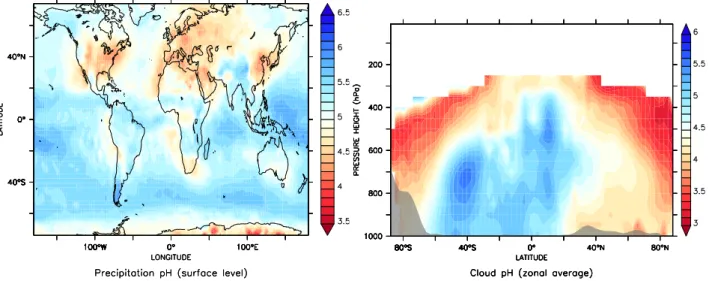
The left panel of Fig. 5 depicts the annual average precipi-tation pH at the surface, originating from both convective and large-scale rainfall, weighted with the amount of rainwater
Fig. 5. Annual average precipitation pH at the surface from large-scale and convective precipitation (left) and annual zonal average of the
cloud pH (right).
and the fraction of the precipitation type. The precipitation pH varies between values around 3.5 and 6.5, being always in the acidic regime due to the atmospheric CO2. Highest
pH values are found over the tropical oceans where pollution sources are small and precipitation rates are high. This is also valid for other regions where pollution is low. In some regions the neutralising effect of ammonia plays a significant role, e.g over India, mainly neutralising the nitric acid pro-duced from intense NOxemissions. The alkaline compounds
of sea salt and mineral dust are neglected in this study, be-cause the ionic composition of these aerosol types is not yet considered in the aerosol submodel M7.
Therefore, the relatively high pH values in the southern storm tracks result mainly from being far from pollution sources. Over the tropical continents, especially Central Africa, the relatively low pH is mostly a result of the NOx
emissions by biomass burning. In several desert regions, e.g. in Africa, the pH can be rather low, mainly due to the small total amount of cloud and rain water, which concentrates the available acidity. In Europe, China and the eastern USA strong anthropogenic emissions of SO2and NOxreduce the
pH of clouds and precipitation, only partly compensated by the dissolution of ammonia.
As mentioned earlier, the comparison with observations can only give indications to what extent the main features and average pH ranges are captured by the model. The cal-culated pH values are compared with observed precipitation pH for the year 2000 in the USA with data from the NADP network (figures in Sect. 2 in the supplement). Even though the main features, e.g., the east-west gradient, are captured well, the correlation is moderate (R≈0.65) and some of the fine structures apparent from the relatively dense network are not resolved. Furthermore, the east-west gradient in the USA is stronger in the observations with values larger than 5 in
the western and central USA, where the model results indi-cate too acidic precipitation. This may partly result from a slight underestimation of the total precipitation, especially in the Central USA, but mostly an overestimation of the H3O+
concentrations. Since sulphate, nitrate and ammonium depo-sition are calculated accurately, we suspect a contribution by mineral cations in wind blown dust and alkaline sea salt, not included in our model setup.
For Europe we use the data collected in the EMEP/CCC Report 1/20068, and the comparison with the simulation indi-cates general agreement with precipitation pH distributions; however, the model is often slightly too acidic. This is partly a consequence of the underestimate of dissolved NHx
(Ta-ble 3). Even though the precipitation distribution in general is captured quite accurately by the model (Hagemann et al., 2006; Tost et al., 2006b) the local variability at specific mea-surement stations can show substantial differences compared to the model grid box average, which affects the rain wa-ter pH. Safai et al. (2004) use a compilation of pH samples for India with average values between 5.3 and 7.7, in rela-tively good agreement with the model simulated results. Ad-ditionally, data by Aikawa et al. (2001) with average precip-itation pH values of 4.7 correspond to the simulation results for Japan.
The right panel of Fig. 5 depicts the annual and zonal av-erage of cloud pH. Above 250 hPa in the tropics to 400 hPa at the poles the liquid water content of the clouds is too small to calculate cloud chemistry, and therefore pH calcu-lations have little meaning, since the clouds consist mainly of ice. The grey shaded area near the lower boundary rep-resents the zonal mean surface orography. The highest pH values are found in the convective regions of the tropics and
in the southern hemisphere storm tracks. The figure shows that the deep convective towers are less acidic due to the high water content and the remoteness from acidic emissions compared to the mid-latitudes. Furthermore the composite of large-scale and convective clouds in the southern storm tracks shows a pH maximum at about 700 hPa, where the liquid water content (LWC) is typically highest, and these re-gions are also remote from acid precursor emissions. In the northern hemisphere the clouds are much more acidic from the surface up to 700 hPa due to anthropogenic emissions of SO2and NOx. The pH values slightly increase toward 600–
700 hPa related to the maximum LWC. The convective ac-tivity north of 40◦N coincides with slightly lower pH values at about 800 hPa compared to the subtropical regions further south where subsidence is dominant. At higher altitudes and further poleward in both hemispheres the clouds are increas-ingly frozen, thus reducing the cloud LWC. Therefore the relatively small amounts of HNO3or H2SO4lead to stronger
acidification under these conditions. However, it should be mentioned that the convective cloud pH is partly too low be-cause we do not use the total convective cloud water for the scavenging calculations but rather the fraction that produces precipitation, since the total cloud water is not directly ac-cessible from the currently used convection parameterisation due to a highly simplified cloud microphysics.
Measurements of pH values in clouds result mainly from hill cap clouds and fog at elevated observatories. Marinoni et al. (2004) measured levels mainly between 4.5 and 5.5 at a remote site in France, but note that there are local NHx
sources. However, at the same site values between 4.1±0.5 and 5.7±0.1 also occur (Sellegri et al., 2003), indicating the high variability. Moore et al. (2004) report pH values for New York between 2.7 and 3.7, thus highly acidic. Of course, such acidic values do not appear in the zonal average, but close to the surface in polluted areas (such as the eastern USA) a similar pH range is calculated by the model.
The pH distribution of the simplified aqueous phase mech-anism (SCM) results in similar patterns. However, these are not identical due to the additional chemical processes in the liquid phase and the feedback via the gas phase (cf. Sec-tion 4.3). Since in the EASY simulaSec-tion dissociaSec-tion reac-tions in the liquid do not take place, a pH value cannot be determined, whereas in EASY2 it is prescribed to calculate the effective Henry’s law coefficients.
4.3 Influences of cloud and precipitation chemistry on gas phase constituents
To analyse the influence of comprehensive aqueous phase chemistry on gas phase constituents, the sensitivity simu-lations described in Sect. 3 are compared for several gas phase species, using the COM simulation as a reference and showing absolute differences to this reference for the other simulations. Furthermore, we evaluate which sim-ulations agree best with the observational data compiled
by Emmons et al. (2000, and references therein)9. For these comparisons only four selected locations are pre-sented here, i.e. from the TOPSE (Atlas et al., 2003) and TRACE-P (Jacob et al., 2003) campaigns, because these measurements approximately coincide with the period for which the applied emission data are representative. We pro-vide additional comparisons with previous campaigns in the electronic supplement (http://www.atmos-chem-phys.net/7/ 2733/2007/acp-7-2733-2007-supplement.pdf). The general evaluation of the tropospheric and stratospheric chemistry in ECHAM5/MESSy1 has been presented by J¨ockel et al. (2006) and Pozzer et al. (2007). Due to the coupling of gas phase chemistry with the cloud and precipitation chemistry we expect direct and indirect effects resulting from a dif-ferent treatment of the aqueous phase chemistry. It should be noted that the terms of direct and indirect effects used here may not be mistaken for direct and indirect aerosol ef-fects on climate. The direct effect in this study is caused by a difference in the uptake into the droplets which depends on the process formulation and the concentration in the liq-uid phase. Furthermore, the consideration of various chem-ical reactions in the liquid may also be conceived as a di-rect effect. The didi-rect effects are especially important for the species participating in comprehensive aqueous phase chem-ical reactions, e.g., SO2conversion to SO2−4 in the droplets
by H2O2and O3, dependent on the pH. Additionally, pH
de-pendent acid-base equilibria are associated with changes in liquid concentrations, if more species are considered.
Furthermore, a different chemical composition of the at-mosphere resulting from cloud and precipitation chemistry modifies the oxidation capacity of the atmosphere, which in-directly alters the mixing ratios of chemically active trace constituents. This is shown by the OH distributions in the supplement (Sect. 4.1, http://www.atmos-chem-phys.net/7/ 2733/2007/acp-7-2733-2007-supplement.pdf). Even though the mixing ratio differences to the reference simulation are relatively small, they indicate that the net turnover of hy-droxyl radicals can increase substantially.
An additional aspect of even higher significance is the modified vertical transport behaviour in convective clouds. In case of a weaker scavenging due to less efficient uptake into the droplets, species with high mixing ratios at the sur-face are more efficiently transported into the upper tropo-sphere, where they can alter the chemical reaction pathways. For a more detailed analysis in addition to the near surface mixing ratios the annual zonal average mixing ratios can be found in the supplement, as well as figures comparing the total global tracer mass. Since the NOSCAV simulation is unrealistic, because of the neglected scavenging and wet de-position, these respective figures have been transferred to the supplement.
9updated dataset obtained from: http://acd.ucar.edu/∼emmons/
4.3.1 Nitric Acid (HNO3)
The surface mixing ratio of HNO3in the COM simulation,
depicted in the upper left panel of Fig. 6, shows highest values in regions with strong NOxemissions caused by the
rapid chemical transformation of NO2 by OH during
day-light and heterogeneous removal of N2O5during night time.
The NOx emissions by industry and traffic (Europe, USA,
China, partly India), soil emissions (tropical rain forests), biomass burning (e.g. Central Africa), all significantly con-tribute to the surface mixing ratios of HNO3. Lightning as
a NOx source is more important in the upper troposphere.
Scavenging and subsequent wet deposition is the main sink of HNO3, being much more efficient than dry deposition and
photodissociation. In the SCM simulation (upper right panel of Fig. 6) similar nitric acid mixing ratios near the surface are computed. Only in the eastern USA and Europe slightly higher values are calculated, whereas almost everywhere else the differences to COM are rather small. The differences mainly result from the indirect effects (higher NOx mixing
ratios (see supplement) due to the neglect of scavenging of HONO and HNO4in SCM) and to a lesser extent from
inter-actions with sulphur compounds in the aqueous phase. The reduced scavenging in EASY, neglecting the dissocia-tion of HNO3in the liquid, leads to higher near-surface
mix-ing ratios worldwide. However, due to the high solubility an important fraction of nitric acid is nevertheless scavenged and removed from the atmosphere by wet deposition. The largest differences occur in the regions with highest overall mixing ratios, emphasising the underestimation of precipita-tion loss by simplified scavenging, whereas in regions remote from the sources the differences are mostly small. Neverthe-less, in this simulation the nitric acid is on average substan-tially higher than in the other setups. The near surface mix-ing ratios in the EASY2 simulation are very close to those of COM (lower right panel of Fig. 6). This emphasises that the concept of effective Henry’s law coefficients is in general applicable for species that mainly dissociate and are only of minor importance for aqueous phase chemistry. The assumed pH of 5 is within the range of that expected (varying from 3.5 to 6, cf. Fig. 5). Thus the scavenging of nitric acid, which almost completely dissociates into nitrate above a pH value of 1, is approximated sufficiently well. On the other hand it should be noted that, even though the near surface mix-ing ratios and also the zonal average distribution of gaseous nitric acid in EASY2 are very close to the COM setup, the nitrate wet deposition in EASY2 is substantially higher than in COM and the observations (cf. Table 4). Additionally, the dry deposition of HNO3 is larger in the EASY2 setup,
both indicating that due to the altered oxidation capacity in EASY2 more HNO3is produced and subsequently removed
by dry and wet deposition.
In the NOSCAV simulation almost everywhere unrealis-tically enhanced HNO3 mixing ratios are calculated near
the surface (see supplement Sect. 5, panel c). In regions
with strong sources the differences are largest, although they propagate over large distances due to the enhanced lifetime. Compared to EASY, the absolute values of the differences to COM are slightly smaller resulting from the more efficient vertical transport due to the neglect of depletion by clouds and precipitation. The global mass of nitric acid is very sim-ilar for COM, SCM and EASY2, showing that the sink pro-cess of wet removal is simulated acceptably with the simpli-fied chemistry, whereas EASY and - much worse - NOSCAV substantially overestimate the HNO3 content of the
atmo-sphere.
The calculated HNO3 mixing ratios for TOPSE and
TRACE-P for both the COM and SCM simulations are well within the range of the observations (Emmons et al., 2000), whereas EASY and much worse NOSCAV strongly overes-timate the HNO3mixing ratios. In EASY2 the HNO3
val-ues are only slightly higher than in COM and SCM. The computed vertical distributions typically indicate a C-shape profile resulting from the NOxemissions at the surface and
downward transport of HNO3 from the stratosphere. Since
the vertical resolution in the tropopause region in the L31 model configuration is relatively coarse, cross-tropopause transport is not represented as well as in the L90 setup of J¨ockel et al. (2006), leading to an overestimation of the in-flux into the troposphere from above. Since no upper bound-ary condition for NOx, HNO3or O3has been applied, which
would mask some of the effects of the cloud chemistry due to enhanced influx from this boundary, the poor representation of the stratosphere and its chemical structure is mainly re-sponsible for the overestimation near the tropopause. For the TRACE-P measurements, in regions where the tropopause is located at higher altitudes and the stratospheric influence at 12 km altitude is less important, this C-shape is less evident. For nitric acid, being hardly chemically active in the liquid phase, except for its almost complete dissociation, the atmo-spheric content and the wet deposition can be simulated with simplified chemistry as well as with an effective Henry’s law equilibrium.
4.3.2 Ozone (O3)
Figure 8 presents the annual average surface mixing ratio of ozone of the COM simulation in the upper left panel. The results from the COM simulation near the surface are very close to those presented in the O3evaluation by J¨ockel
et al. (2006), showing relatively high mixing ratios in Cali-fornia (e.g. Jacobson, 2005), the Mediterranean region (e.g. Lelieveld et al., 2002), around the Persian Gulf (resulting from high propane emissions), northern India and the Hi-malayas (the latter associated with the strong surface ele-vation). The absolute differences between the SCM and COM simulations, depicted in the upper right panel of Fig. 8, mostly result from indirect effects, in particular via the removal of nitrogen oxides. Nevertheless, direct chemi-cal effects through reduced O3formation and enhanced O3
(a) HNO3surface layer (b) absolute difference
mixing ratio (nmol/mol) (COM) (nmol/mol) (SCM-COM)
(c) absolute difference (d) absolute difference
(nmol/mol) (EASY-COM) (nmol/mol) (EASY2-COM)
Fig. 6. Comparison of the annual average HNO3surface layer mixing ratio for the four sensitivity simulations: shown is the absolute value
for the COM simulation (upper left panel) and – as indicated – the absolute differences of the other simulations to the COM simulation.
Fig. 7. Comparison of the HNO3vertical profiles compiled by Emmons et al. (2000) with the results of the five sensitivity simulations. The observations are depicted by the black points, their variability (standard deviation) by the black boxes and the number of points taken into account for this campaign (in space and time for this region) are listed at the right axis. The model results are represented by the solid lines and the respective standard variation by the triangles. The colours denote the simulations as indicated in the legend, i.e., red = COM, green = SCM, blue = EASY, turquoise = EASY2 and magenta = NOSCAV.
(a) O3surface layer mixing (b) absolute difference
ratio (nmol/mol) (COM) (nmol/mol) (SCM-COM)
(c) absolute difference (d) absolute difference
(nmol/mol) (EASY-COM) (nmol/mol) (EASY2-COM)
Fig. 8. Comparison of the annual average O3surface layer mixing ratio for the four sensitivity simulations, displayed similarly as in Fig. 6.
destruction in clouds play a secondary role over parts of the eastern USA, western Europe, South America and near Japan. On the other hand, in eastern Europe and near In-donesia and the Indian Ocean detailed cloud chemical pro-cesses enhance ozone mixing ratios near the surface, mostly because chemical destruction pathways of O3 are reduced.
The indirect effects of the cloud chemistry result mainly from the modified NOx mixing ratios. Consequently, the ozone
production from NOx (ProdNo, shown in the supplement)
is altered: in regions where the modified scavenging/cloud chemistry formulation leads to enhanced NOxalso enhanced
O3is found and vice versa. The influence of aqueous phase
chemistry on the other major ozone production and destruc-tion rates is lower. The ozone mixing ratios computed in the EASY simulation are predominantly higher than in COM, largely resulting from the less efficient removal of O3
pre-cursor gases. This results in relative increases of up to about 20% at some locations, as shown in the lower left panel of Fig. 8, whereas in Europe and near Indonesia the reduction of O3loss is more important. With the effective Henry’s law
equilibrium in EASY2 (lower right panel of Fig. 8) the dif-ferences to COM are much smaller than in EASY, but overall slightly more O3is simulated in the surface layer, again
re-sulting mainly from indirect effects. The simulation without cloud processes and scavenging (NOSCAV) generally results in much higher and unrealistic O3mixing ratios throughout
the troposphere, resulting from the drastically altered con-centrations and distributions of precursor gases. Unquestion-ably, the cloud and precipitation related chemistry and re-moval processes yield much reduced oxidant levels in the gas phase.
Figure 9 presents a comparison of model results with air-craft observations. From the TOPSE measurements an in-crease of O3mixing ratios with altitude near the tropopause
illustrates the influence of stratospheric O3. For the lower
and middle troposphere the COM, SCM, EASY2 and EASY simulations produce rather similar results, being close to the measurements, while the EASY results for O3 are
system-atically higher. The NOSCAV simulation strongly overesti-mates O3 mixing ratios throughout the troposphere, and is
unable to reproduce the observations. In general, the ob-servations are reproduced quite accurately by the COM and SCM simulations, although for Hawaii all simulations over-estimate O3, with COM and SCM being slightly lower. In the
upper troposphere in the model the influence of the strato-sphere appears to be too strong, resulting from an overesti-mated transport into the troposphere due to the coarse ver-tical resolution. J¨ockel et al. (2006) show that this process is simulated quite realistically using the model configura-tion with enhanced vertical resoluconfigura-tion near the tropopause (90 vertical levels).
4.3.3 Hydrogen peroxide (H2O2)
Hydrogen peroxide (H2O2) efficiently dissolves into the
liq-uid phase, where it can oxidise S(IV) and is removed from the atmosphere by precipitation. Because of the much lower solubility of OH, NO3 and other oxidants, it is a main
oxi-dant in the liquid phase. The oxidation reactions represent an additional chemical sink of this compound in clouds and precipitation.
This is illustrated in Fig. 10, in which the annual aver-age surface mixing ratio of H2O2is displayed for the COM
simulation (upper left panel). Relatively high values occur over the tropical rainforest regions, associated with abun-dant NMHC oxidation with high yields of the main precur-sor of hydrogen peroxide, i.e., hydroperoxy radicals (HO2).
Toward the poles a strong negative gradient is evident, re-lated to both the lower NMHC emissions and lower photo-chemical activity. In the upper right panel with the reduced chemical mechanism (SCM) higher values than in COM are calculated in the tropics. Since in this setup the photoly-sis of H2O2in the aqueous phase, representing a chemical
loss process, is neglected, the liquid phase concentrations are higher than in COM and the uptake into droplets is less ef-ficient. In eastern Europe the mixing ratio near the surface in SCM is lower than in COM, resulting mainly from the al-tered chemical composition (indirect effect), whereas in the polar regions with low mixing ratios the absolute differences are small. The indirect effect results mainly from the en-hanced ozone mixing ratios, producing more OH and HO2,
and consequently more H2O2.
The lower left panel, presenting the EASY simulation, in which the liquid phase oxidation of SO2is additionally
ne-glected, the differences are larger. In the polluted regions of the northern hemisphere (eastern USA, western Europe, China) substantially higher H2O2 mixing ratios are
calcu-lated due to this neglect. The EASY2 simulation shows very similar average near surface mixing ratios for H2O2, since
the processes in which hydrogen peroxide is involved are al-most identical. This results in a comparable distribution as in EASY. However, especially over China in both model se-tups based on a Henry’s law equilibrium substantially higher H2O2 mixing ratios are calculated due to the missing SO2
oxidation.
The vertical distribution for the five simulations (Sect. 6.1 of the supplement) shows highest differences close to the surface in the tropics. In the middle troposphere these dif-ferences are smaller, and in the upper troposphere they are hardly discernable for SCM, EASY or EASY2. This is mainly based on the H2O2photolysis in the gas phase which
becomes more efficient with altitude. However, close to the surface the photolysis in the liquid phase has substantial ef-fects producing the lower mixing ratios in the COM simula-tion compared to the sensitivity studies. Due to the vertical mixing in the troposphere, the higher mixing ratios of the
(a) H2O2surface layer mixing (b) absolute difference
ratio (nmol/mol) (COM) (nmol/mol) (SCM-COM)
(c) absolute difference (d) absolute difference
(nmol/mol) (EASY-COM) (nmol/mol) (EASY2-COM)
Fig. 10. Comparison of the annual average H2O2surface layer mixing ratio for the four sensitivity simulations, displayed similarly as in
Fig. 6.
sensitivity studies are transported upwards into the middle troposphere as mentioned above.
In the NOSCAV simulation (see Sect. 5 of the supple-ment), the missing sink of wet deposition leads to slightly higher mixing ratios compared to the reference in the po-lar and the marine subsidence regions, whereas in almost all other locations the values are lower (most obvious over the tropical continents, but also over parts of the oceans, e.g., the SPCZ). These regions are strongly influenced by convective activity, in which the missing wet removal results in an en-hanced upward transport into the upper troposphere which is not balanced by downward transport within the aqueous phase. The vertical distribution (see supplement) indicates higher mixing ratios by more than 50% compared to the COM simulation.
Additionally, among the indirect effects it must be consid-ered that over the tropical continents the simplified and there-fore underestimated wet removal results in higher mixing ra-tios of organic compounds. These species can partly deplete OH and HO2by oxidation processes (e.g., since CH3OOH
is not scavenged in NOSCAV the HOxmixing ratios are
re-duced (see reactions G4107 and G4103 in supplement). In case of a complete neglect of scavenging those effects are even stronger. Consequently, less H2O2is formed from the
self reaction of HO2. Due to the low NOx mixing ratios
in these remote regions a recycling of the oxidants is not as efficient as in the polluted regions of the northern hemi-sphere. Consequently, the total global mass of H2O2is by
far highest in NOSCAV throughout the middle and upper troposphere, whereas EASY, EASY2 and SCM calculate a similar atmospheric burden. Since all sensitivity simulations with simplified cloud and precipitation chemistry calculate higher mixing ratios of H2O2, this compound contributes to
enhanced OH production through its photodissociation in the gas phase, and therefore accelerates the gas phase chemistry (contributing through indirect effects).
This is also supported by the comparison with obser-vations in Fig. 11. The vertical profiles for COM and SCM are very similar for the TOPSE campaign. EASY2 shows slightly enhanced mixing ratios, whereas EASY and NOSCAV result in substantially higher values. However, close to the surface in NOSCAV nearly comparable low val-ues are calculated. For the TRACE-P data in China and Hawaii, COM is slightly lower than SCM. The EASY sim-ulation is characterised by the highest values in the lower troposphere, but NOSCAV, being similar or lower than COM close to the surface, yields significantly higher H2O2values
than the other simulations above 2 km altitude. As expected, the NOSCAV simulation does not reproduce the measured H2O2mixing ratios, and strongly overestimates the mixing
ratios at altitudes above 2 km. Similarly, in the EASY simu-lation the missing sinks by aqueous phase chemistry result in an overestimation relative to the observations. EASY2 calcu-lates higher values than COM and SCM, but still lower than EASY. This is mainly restricted to the lower and middle
tro-posphere, whereas in the upper trotro-posphere, in which only small amounts of liquid water are available for chemical re-actions in droplets, the differences between the simulations including the wet removal are smaller because of the rapid photolytical destruction. The COM and SCM simulations both lead to too high mixing ratios compared to the TOPSE data, although they are in reasonable agreement with the TRACE-P data, with the mean value well within the range of the measurements.
We conclude that for a realistic description of lower and middle tropospheric H2O2 mixing ratios at least the basic
cloud and precipitation chemistry of this compound must be included in the model (i.e., SCM). An enhanced scavenging coefficient, i.e. larger than expected from Henry’s law equi-librium, might be used as an approximation, but this cannot be determined easily for all conditions in the troposphere. Additionally, such an approximation suppresses important chemical feedbacks.
4.3.4 Sulphur dioxide (SO2)
Since SO2is relatively short-lived, the distribution near the
surface, presented in Fig. 12, shows strong gradients with the highest values close to the emission centres, i.e. Europe, east-ern China, and additionally the easteast-ern USA, India, Saudi-Arabia and Chile. Over the ocean the DMS (dimethylsul-phide) oxidation and to a lesser extent ship emissions result in average mixing ratios of less than 0.5 nmol/mol. In case of a reduced aqueous phase chemistry as in the SCM sim-ulation, in which the main oxidation of S(IV) to S(VI) by H2O2and O3is nevertheless considered, the differences to
the reference are relatively small except in the heavily pol-luted regions near the strongest SO2 sources. This results
mainly from the altered H2O2mixing ratios, and the
conse-quent changes in oxidant mixing ratios (indirect effect), but also from the more detailed sulphur chemistry in the aqueous phase, e.g., interactions between oxidised sulphur and nitro-gen compounds (direct effect). Overall, in SCM this leads to slightly enhanced SO2mixing ratios compared to COM,
both close to the surface and at higher altitudes.
In the EASY simulation the aqueous phase oxidation of sulphur dioxide is neglected, i.e., a main chemical sink is missing, and the scavenging is less efficient as in SCM or COM. This leads to globally higher mixing ratios, most strongly in the regions near the emission sources. In EASY2 the dissociation of SO2 in the liquid is taken into account,
but the liquid phase oxidation is still not considered. This cannot be easily parameterised with the help of a coefficient since it depends not only on the pH, but also on the dissolved oxidant concentrations, which show large variability in time and space (e.g., H2O2, cf. Fig. 10). Consequently, the
atmo-spheric content of sulphur dioxide is still overestimated and the sulphate wet deposition is underestimated (cf. Table 4).
In the NOSCAV simulation higher mixing ratios at the sur-face are calculated, too, but in this case they are not as high as
(a) SO2surface layer (b) absolute difference
mixing ratio (nmol/mol) (COM) (nmol/mol) (SCM-COM)
(c) absolute difference (d) absolute difference
(nmol/mol) (EASY-COM) (nmol/mol) (EASY2-COM)
Fig. 12. Comparison of the annual average SO2surface layer mixing ratio for the four sensitivity simulations, displayed similarly as in
Fig. 6.