HAL Id: hal-01015204
https://hal.archives-ouvertes.fr/hal-01015204
Submitted on 1 Jul 2014HAL is a multi-disciplinary open access archive for the deposit and dissemination of sci-entific research documents, whether they are pub-lished or not. The documents may come from teaching and research institutions in France or abroad, or from public or private research centers.
L’archive ouverte pluridisciplinaire HAL, est destinée au dépôt et à la diffusion de documents scientifiques de niveau recherche, publiés ou non, émanant des établissements d’enseignement et de recherche français ou étrangers, des laboratoires publics ou privés.
Investigation of the time variability of diurnal tides and
resonant FCN period
Xiaoming Cui, Heping Sun, Séverine Rosat, Jian-Qiao Xu, Jiang-Cun Zhou,
Bernard Ducarme
To cite this version:
Xiaoming Cui, Heping Sun, Séverine Rosat, Jian-Qiao Xu, Jiang-Cun Zhou, et al.. Investigation of the time variability of diurnal tides and resonant FCN period. Journal of Geodynamics, Elsevier, 2014, pp.GEOD-1307. �10.1016/j.jog.2014.05.003�. �hal-01015204�
Investigation of the time variability of diurnal tides and resonant FCN period
Xiaoming Cuia, Heping Suna, Séverine Rosatb , Jianqiao Xu a, Jiangcun Zhoua, Bernard Ducarmec a State Key Laboratory of Geodesy and Earth's Dynamics , Institute of Geodesy and Geophysics, CAS,
Wuhan, China,430077
b Institut de Physique du Globe de Strasbourg (UMR 7516 CNRS, Université de Strasbourg/EOST), 5
rue René Descartes, 67084 Strasbourg Cedex, France
c Georges Lemaître Centre for Earth and Climate Research, Catholic University of Louvain,3 Chemin du
Cyclotron,1348 Louvain-la-Neuve, Belgium
Abstract: The time variability of diurnal tides was investigated by analyzing gravity observations
from global superconducting gravimeter (SG) stations with running time intervals. Through least-square and Bayesian approaches, FCN resonance parameters were estimated for each data section after obtaining the tidal parameters of mainly diurnal tidal waves. The correlation of the time variation in diurnal tidal waves and FCN period was discussed. For comparison, a similar method was used to analyze VLBI observations to study the time variability of nutation terms and FCN period. The variation trend of the FCN period totally depends on the Ψ1 wave in tidal gravity and on the retrograde annual term in nutation. We observed a similar variation trend in the FCN periods obtained from different SG stations worldwide and VLBI observations. The relation between diurnal tides and LOD variations is discussed and the possible mechanisms of the decadal variation in FCN periods were discussed.
Keywords: Temporal Variation, Superconducting Gravimeter, Diurnal Tides, VLBI, FCN
1. Introduction
Due to the interaction between the elliptical liquid core and the solid mantle of the Earth, a retrograde rotational mode called the Free Core Nutation (FCN) occurs in the celestial reference frame, appearing as a nearly diurnal free wobble (NDFW) in the terrestrial reference frame. The period of FCN strongly depends on the flattening of the core–mantle boundary (CMB) and can also be influenced by other coupling mechanisms, such as visco-electromagnetic and topographic coupling. As the most active thermal boundary layer inside the earth, the CMB is typically accompanied by changes in physical characteristics and structure which will possibly affect those coupling mechanisms and then may cause some variations in the FCN period.
FCN parameters (period and quality factor) can be estimated by the resonance enhancement in observations of earth tidal waves or nutation terms with frequencies close to its eigenfrequency. The most commonly used data are high-precision time-varying gravity observed by superconducting gravimeters (SGs) and nutation observations from VLBI network analysis. The FCN resonance parameters can also be inverted from strain data (e.g. Amoruso et al. 2012). The usual approach in determining FCN parameters is linearized least-square method (LSQ) (Defraigne et al., 1994; Sun et al., 2004). Florsch and Hinderer (2000) proposed a Bayesian approach that more effectively solves non-linear inverse problems. The temporal variation in FCN period has been investigated through VLBI and SG observations in numerous previous works. Some of these studies (Roosbeek et al., 1999; Hinderer et al., 2000; Lambert and Dehant, 2007; Vondrak & Ron, 2009) found no evidence of variation in the FCN period, whereas Xu and Sun (2009) showed a decadal temporal variation in the FCN period by analyzing long SG records at Brussels station. This problem remains a matter of dispute. Conclusions are difficult to draw when only one kind of observation is made because
observed variations are small (sometimes within error bars).
The accumulation of SG data offers a good opportunity to perform the study by comparing the results from two different techniques. The Global Geodynamics Project (GGP) sponsored and organized by the Solid Earth’s Deep Interior (SEDI) in IUGG in 1997, has accumulated more than 10 years of observations at many global SG stations, and especially, over 20 years of SG observations in Strasbourg station (France). In studying the temporal variation of the FCN period, observations from different SG sites can be compared to check the reliability of the variation as well as with VLBI observations.
In this paper, based on observations from seven SG stations, we use running time intervals to conduct tidal analyses and estimate FCN parameters section by section. We then compare the variations of the FCN period with those of the amplitude factors of some diurnal tidal waves. Similarly, we analyze VLBI observations and study the transfer function values of nutation terms used to determine FCN parameters and their relation with the variations of the FCN period. We also focus on the differences by using different datasets (SG and VLBI) and approaches (LSQ and Bayesian).
In the following sections, we introduce the data, the FCN resonance model, and the determination approaches of FCN parameters. The data analyses and the temporal variations in FCN period are then discussed.
2. Data, FCN model, and parameter determination methods
2.1 Data introduction
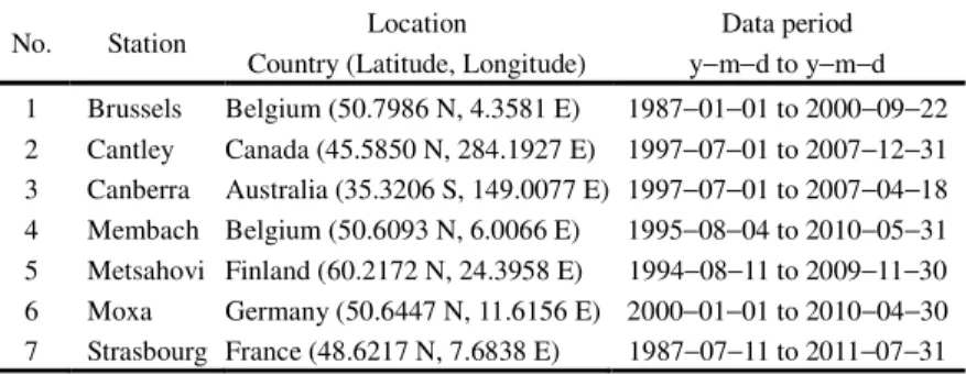
located in central Europe, where ocean tide effects at diurnal frequencies are small and for which we usually obtain high-quality data (e.g. Rosat and Hinderer, 2011) with more stable observation environments. The exception is Brussels site which was quite noisy but for which the data record is interestingly long. Among the five stations, Strasbourg station has the longest-term observations, from 1987 to 2011, which is the main time series we focus on. Other stations are studied for compensation. Considering the possible regional effect, two SG stations in Canada and Australia are also included for comparison. Basic information on each station and data length are listed in Table 1. The VLBI observation used in this study is the IVS combined solution “ivs12q3X” (International VLBI Service for Geodesy & Astrometry) in the form of celestial pole offsets (dX, dY) referred to IAU2006 precession-nutation model (Wallace and Capitaine, 2006) excluding the free core nutation. These data are given in non-equidistant intervals of 1 day to 7 days. We choose the same data length from 1987-07 to 2011-07 as Strasbourg SG observations in our study.
Table 1. Basic information on SG stations and data used in this study
No. Station Location
Country (Latitude, Longitude)
Data period y−m−d to y−m−d 1 Brussels Belgium (50.7986 N, 4.3581 E) 1987−01−01 to 2000−09−22 2 Cantley Canada (45.5850 N, 284.1927 E) 1997−07−01 to 2007−12−31 3 Canberra Australia (35.3206 S, 149.0077 E) 1997−07−01 to 2007−04−18 4 Membach Belgium (50.6093 N, 6.0066 E) 1995−08−04 to 2010−05−31 5 Metsahovi Finland (60.2172 N, 24.3958 E) 1994−08−11 to 2009−11−30 6 Moxa Germany (50.6447 N, 11.6156 E) 2000−01−01 to 2010−04−30 7 Strasbourg France (48.6217 N, 7.6838 E) 1987−07−11 to 2011−07−31 2.2 FCN resonance model
In the terrestrial reference frame, the NDFW will lead to an obvious resonance enhancement in observations of diurnal tidal waves with near frequencies. The FCN parameters are estimated by fitting the observed complex gravimetric factors (complex ratio of the observed tidal amplitude to
the tidal amplitude for a solid Earth model given a tide-generating potential) to a damped harmonic oscillator modeling the resonance. The observed values of gravimetric factors for each tidal wave could be obtained by analyzing SG data (see paragraph 3). For a diurnal tidal wave of frequency σ,
complex gravimetric factors can be described as follows (Hinderer et al., 1991):
0 j j nd a δ δ σ σ = + − , (1)
where δ0 is the gravimetric factor independent of the frequency and not influenced by the resonance,
a
~
is the complex resonance strength related to the geometric shape of the Earth and therheological properties of the Earth’s mantle, and σnd
~ is the complex eigenfrequency of the NDFW.
Denoting I
nd R nd
~ σ σ
σnd = +i , and
a
~
=
a
R+
ia
I , where R and I represent the real and imaginary parts,respectively. The quality factor Q and the FCN eigenperiod TFCN are expressed as I nd R nd/ 5 . 0
σ
σ
= Q and FCN /( ) R ndT = Ω σ + Ω , where Ω is the sidereal frequency of the Earth’s
rotation.
In the celestial reference frame, the resonance of the liquid core affects the Earth’s nutation as well. The resonance for a nutation term with frequency σ, usually represented by a transfer function,
can be expressed as follows (eqs.(42) in Mathews et al., 2002):
4 0 0 1 ( ) 1 (1 )( ) 1 R R Q e T N Q e s α α α σ σ σ σ = − = + + + ∑ − − , (2)
where eR is the dynamic ellipticity of the rigid earth; s1, s2, s3, and s4respectively represent the
frequencies of the Chandler Wobble, FCN, Free Inner Core Nutation and Free wobble of the inner core; N0 and
0
Q
are constants defined in Table 6 of Mathews et al. (2002); andQ
α are
resonance strengths of the respective rotational modes.
The main diurnal tidal waves usually employed to estimate FCN parameters include P1, K1, Ψ1, and Ф1, in which Ψ1 is the closest in frequency to the NDFW and thus has the most significant
amplitude enhancement. For nutation, thousands of nutation terms are involved in the MHB2000 nutation model (Mathews et al., 2002). Only those terms with frequencies close to the FCN frequency and with large amplitudes are important to determine the FCN parameters, such as the 365.26 day (l’), 182.62 day (2F-2D+2 ), 121.75 day (l’+2F-2D+2 ), 27.55 day (l), and 13.66 day (2F+2 ) nutation terms, where l, l’, F, D, and correspond to the Delaunay variables characterizing the nutation terms.
As we know, each nutation term with an elliptic orbit can be expressed as the sum of two circular terms which have identical frequencies with opposite signs. Due to the same gravity potential source (mainly degree 2 and order 1 component in the spherical harmonic decomposition of the tide-generating potential), a corresponding relationship exists between the tidal waves and the nutation terms. Hence, the Ψ1 wave corresponds to the retrograde annual nutation term (–365.26 days), which is the closest to the FCN, and the two terms should be most sensitive to any variation of FCN frequency. If some temporal variations in the FCN period exist, the diurnal tidal waves or nutation terms near the FCN would be sometimes closer and sometimes farer to the resonance, in
pace with the variations. As a consequence, the amplification of these waves or nutation terms would
vary according to the resonance model (1) or (2).
2.3 Review of the linearized least-squares and Bayesian approaches
The estimation of FCN parameters consists in solving a non-linear inverse problem. The approach mostly used in previous work is a linearized LSQ method optimized by the Levenberg–Marquardt algorithm (Marquardt, 1963). Equations (1) and (2) are used to construct the merit function and to evaluate unknown parameters by an iterative process given initial values. For
nutation, we directly use Equation (2) as the calculation model. However, for earth tidal waves, we usually use the observed O1 wave as a reference (e.g., Defraigne et al., 1994; Ducarme et al., 2007) to reduce the effects of any systematic discrepancies (e.g., calibration errors) or local environmental disturbances in the fitted resonance parameters of the FCN. The O1 wave has a relatively large amplitude and high signal-to-noise ratio and is minimally influenced by FCN resonance, so it can be observed very accurately. Subtracting the contribution of O1 from both sides of Equation (1) yields
nd O nd j O j a a σ σ σ σ δ δ~ ~ ~~ ~ ~ 1 1 − − − = − . (3)
The values of the unknown parameters (
a
~
andσ~
nd) are optimal when the merit function f is minimal. The function f can be written as[
]
2 1 1 ~ ~ ~ ~ ~ ~ ) ( − − − − − =∑
nd O nd j O j a a p f σ σ σ σ δ δ σ σ , (4)where p(σ) is the weight function of tidal parameters with frequencies σ.
The Bayesian method has been shown to be more suitable for the inversion of non-linear problems (Tarantola and Valette, 1982a). It can make full use of the data information combined with some prior information on the data or on the unknown parameters. Based on these advantages, the Bayesian approach has been proposed to estimate FCN parameters (Florsch and Hinderer, 2000; Rosat et al., 2009).
As the quality factor Q of the FCN expresses signal damping caused by any kinds of dissipative processes, the value of Q should be positive. For earth tidal waves, a priori information x=log10Q is involved to retain the positivity of Q in Equation (1). The real and imaginary parts of the amplitude factors are written as follows:
0 2 2 2 2 ( ) (( 10 ) / 2) Re( ) ( ) (( 10 ) / 2) ( ) (( 10 ) / 2) Im( ) ( ) (( 10 ) / 2) R R I R x j nd nd th j R R x j nd nd I R R R x j nd nd th j R R x j nd nd a a a a
σ
σ
σ
δ
δ
σ
σ
σ
σ
σ
σ
δ
σ
σ
σ
− − − − − − = + − + − + = − + . (5)For detailed information on the construction of the Bayesian calculation scheme, we refer to Tarantola and Valette (1982a,b) and Florsch and Hinderer (2000). The unknown parameters are described by the probability distribution P (Rosat et al., 2009)
(
)
2 2Re(
)
Im(
)
1
,
,
,
exp
2
th R th I j j j j R R I nd R I j j jP x
σ
a
a
k
δ
δ
δ
δ
δ
δ
−
−
=
−
+
∆
∆
∑
, (6)where k is a normalization factor in order that the integral of this equation is unity;
∆
δ
Rj and∆
δ
Ijare the standard deviations of the real and imaginary parts, respectively, of the gravimetric factors. For the nutations, the Bayesian calculation model can be similarly constructed by representing the “nutational” factors with the transfer function values as in Rosat and Lambert (2009).
3. Temporal variations of the FCN period in SG data
Before fitting the FCN parameters with SG observations, we need to obtain the tidal parameters (amplitude factor and phase lag) of earth tidal waves. All SG data were preprocessed to eliminate any disturbance, such as steps, spikes and earthquakes, to ensure the accuracy of tidal analysis. The tidal parameters were then estimated by analyzing 1-h sampled SG data with the ETERNA (Wenzel, 1996) software. The tidal potential used in the analysis is Hartmann–Wenzel (1995). First, we consider the Strasbourg SG data which are a combination of records from two instruments: the SG TT070-T005 recording from 1987 to 1996 and the SG C026 recording from 1996 to 2011. In order to check for any temporal variations in the FCN period, we analyze the data
1992 1996 2000 2004 2008 -2 -1 0 1 2 3 x 10 -3 Time(year) ∆ δ (Ψ 1 ) Canberra Cantley Strasbourg
section by section using a running time interval with a shifting of 1 year. The length of each data segment should respect the frequency resolution required for separation of the diurnal waves (Q1, O1, P1, K1, Ψ1, and Φ1). In our study, 6-year and 3-year intervals are used and the retrieved delta-factors are plotted with respect to the center of the interval. A 6-year time interval is used only for Strasbourg station because of its sufficiently long series and for subsequent convenient comparison with the VLBI results later. For the VLBI data, a 6-year interval should be used to ensure the separation of the FCN and the retrograde annual nutation terms which are very close in frequency. In surface gravity observations, the FCN cannot be directly observed and separated from the close-by tidal waves because the expected amplitude is very small in the terrestrial reference frame. Therefore, our study mainly focuses on its resonance effect in diurnal tidal waves, and the
FCN period is estimated from the resonance. Nevertheless, we first need to check whether there is
an effect of the wave group separation when the FCN frequency (about 1.00507cpd – cycle per day)
is included or not in the frequency band of the waves (K1 &Ψ1) adjacent to FCN.
Figure 1. Differences in Ψ1 amplitude factors when the Ψ1group contains or not the FCN for 3 SG
When performing tidal analysis with ETERNA software for each 6-year data section of
Strasbourg, we changed the frequency limits for the K1 group in two cases: K1 (1.001824 cpd to 1.004107 cpd) without FCN and K1+FCN (1.001824 cpd to 1.005327 cpd), including FCN.
Similar way
is used for Ψ1 (1.005328 cpd to 1.007594 cpd) and Ψ1+FCN (1.004108 cpd to 1.007594 cpd). For K1, including or excluding FCN has a negligible influence (10-8) to the amplitude factor. Considering that K1 is farther from FCN relatively, we also test the K1x+ waves. The influence is in the order of 10-5 which is one or two orders of magnitude smaller than the standard deviation of K1x+’s amplitude factor. For Ψ1, the difference for the amplitude factor including or excluding FCN is in the order of 10-3 which is in the same order as the Ψ1 standard deviation (cf. Fig. 1). Given that Ψ1 corresponds to the 6-month modulation of S1, we also checkedthe variation in the amplitude factor for S1, and the differences for Ψ1 and S1 are anticorrelated. This indicates that the differences we obtained are real ones and not perturbations on the tidal records because S1 and Ψ1 are respectively associated with the prograde and retrograde annual terms of nutation.
Considering that this influence is at the level of the precision we have on Ψ1, we take the minimum frequency 1.005328 cpd for the Ψ1 group to exclude the FCN in the tidal analysis. Such a difference shall reflect the noise effect. However, we perform a similar test with the SG data at the Canberra and Cantley stations, as shown in Fig 1. The difference for δ(ψ1) including or excluding the FCN at the two stations is consistent with the results obtained for Strasbourg. It is very interesting that the results for the 3 stations located on different continents have a very similar behavior particularly between 1998 and 2007. A reasonable explanation may be that this result is
the combined effect of tiny waves, FCN, or other tidal signals that are not modeled. This effect should be investigated in a further study.
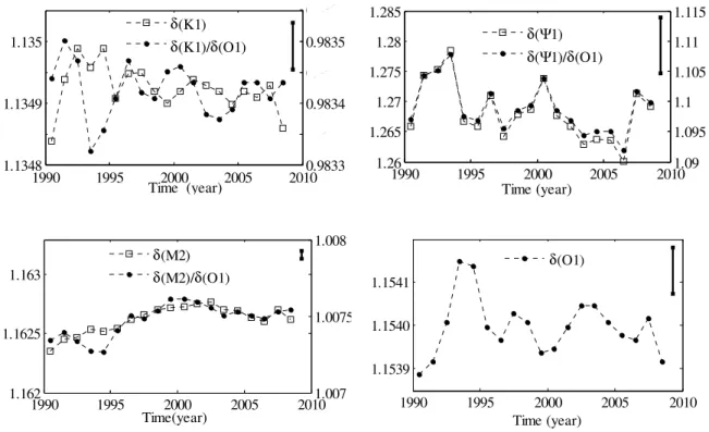
Figure 2. Time-variations of amplitude factors for K1, Ψ1, M2 and relative ratios to O1 at Strasbourg station estimated with ETERNA 3.4 software on 6-year segments shifted by 1 year (the vertical short
line on the top right corner of each graph is the mean standard deviation for each wave; For first 3
figures, left vertical axis represents the amplitude factors for each wave, and right vertical axis represents
their relative ratios to O1). The ocean loading effect has been corrected using FES2004 model.
After testing the influence of the group separation in ETERNA tidal analyses, we can process the Strasbourg data with 6-year segments shifted by 1 year. The correlation between the FCN parameters has been investigated in some previous work (e.g., Florsch & Hinderer, 2000; Rosat et al., 2009). A strong correlation exists between the FCN period and the gravimetric amplitude factor
1.26 1.265 1.27 1.275 1.28 1.285 Time (year) 1990 1995 2000 2005 20101.09 1.095 1.1 1.105 1.11 1.115 δ(Ψ1) δ(Ψ1)/δ(O1) 1.1348 1.1349 1.135 Time (year) 1990 1995 2000 2005 20100.9833 0.9834 0.9834 0.9835 0.9835 0.9836 δ(K1) δ(K1)/δ(O1) 1.162 1.1625 1.163 Time(year) 1990 1995 2000 2005 20101.007 1.0075 1.008 δ(M2) δ(M2)/δ(O1) 1990 1995 2000 2005 2010 1.1539 1.1540 1.1541 Time (year) δ(O1)
of Ψ1. In Fig.2, we plot the time variations of the delta-factors for K1 and Ψ1. The two waves are located at opposite sides of the FCN frequency and should be most sensitive to any variation of the FCN period than other waves. The δi for M2 and O1 are also plotted.
Since the oceanic tides have the same driving mechanism and similar spectral pattern as body tides, it is not possible to separate their effects by harmonic analysis. Therefore the oceanic influence has to be evaluated using an ocean tides model of the different tidal constituents (Melchior et al., 1980). The tidal loading vector, which takes into account the direct attraction of the water masses, the flexion of the ground and the associated change of potential, is evaluated by performing a convolution integral between the ocean tide models and the load Green’s function (Farrell, 1972). According to the principle of vector superposition, the loading effects of oceanic tides can be removed from the obtained gravimetric factors. In this paper, the amplitude factors are corrected for the ocean tide effect on the basis of the Fes04 model (Lyard et al., 2006) and following the computation scheme as in Ducarme et al. (2007).
As mentioned above, the Strasbourg time series was obtained from two different instruments. Therefore, a calibration problem may affect our study. Indeed, the tidal factors from the T005 have been multiplied by a factor of 1.001529 to correct for an observed scale factor error. In order to avoid any contamination from errors in the scale factor and to be free from any possible changes in the sensitivity of the gravimeter, we also plot in Fig. 2 the δi factors for K1, Ψ1, and M2 normalized by the O1 amplitude factor δ(O1).
δ(K1) and δ(O1) are very stable, with a variation less than 0.02%. The variation of δ(ψ1) is larger and about 2%. We can note that the overall variation shape for K1 and Ψ1 is comparatively consistent, especially after normalization to δ(O1). δ(M2) is also very stable with a variation of
about 0. 05%. This stability shows that the multiplication by 1.001529 for the old T005 series was necessary to reach such accuracy on the gravimetric factors.
After the tidal parameters have been corrected from the ocean loading, the FCN period can be determined by the methods introduced in the previous section. We used 5 tidal waves to perform the inversion: O1, P1, K1, Ψ1, and Ф1. The usual weights applied in LSQ or Bayesian methods are the inverse of the standard deviations of the tidal amplitude factors resulting from the ETERNA tidal analyses. In our LSQ inversion, the results show a very large standard deviation of about 10 d to 30 d for the FCN period. This deviation is disadvantageous for our study on its variation trend. We then apply other weights used in Liu et al. (2007) which will significantly reduce the standard deviation of the period. These new weights are inversely proportional to the standard deviations of the amplitude factors and to an additional factor representing the frequency difference between the wave frequencies and the FCN frequency. The two weighting schemes lead to a difference in the FCN period of a few days, but it has no influence on its time variations. Based on the weights of Liu et al. (2007), the standard deviation for the FCN period decreases to a few days. In the Bayesian inversion, we employ the usual weighting scheme.
The results of the Bayesian and LSQ approaches are depicted in Fig. 3. The comparison of the amplitude factors for all diurnal waves shows a strong correlation between the FCN period variations and the δ(ψ1) time fluctuations. In Fig.3, we have also plotted the values of δ(ψ1)/ δ(O1). For the sake of comparison, we have reversed the vertical axis for the relative amplitude factors in Fig. 3. The obtained apparent time-variations of the FCN period differ by a few days between both methods, but the variation trend is similar. We clearly see that the variation trend of the FCN period and of δ(ψ1) are correlated, which is not surprising since the FCN parameters are strongly
1990 1995 2000 2005 2010 410 420 430 440 P e ri o d ( S D ) Bayesian LSQ 1.09 1.1 1.11 Time (year) δ(Ψ1)/δ(O1) Polynomial fitting
dependent on δ(ψ1). Using different weights in the LSQ method does not change the variation trend of the FCN period. By superposing a polynomial fitting curve, we observe a decade fluctuation in δ(ψ1)/δ(O1) and in the FCN period. It is worth to note that it is not precise to fitting a period signal with polynomial curve due to the edge effects, polynomial degrees, etc. But our aim here is to make the variation trend clear and to study the similar variation trend between SG and VLBI results. For further verification, we use intervals of 3 years instead of 6 years for the tidal analyses of the Strasbourg SG data. The resulting Ψ1 amplitude factors are plotted in Fig. 4. The standard deviation of δ(K1) for the old SG T005 series (1987–1996) is in the order of 10-4, whereas for the C026 observations (1996–2011), it is in the order of 10-5. For Ψ1, the order of standard deviation for the two instruments is respectively 10-2 and 10-3. The more recent instrument has obviously a higher observation quality as already mentioned in Rosat and Hinderer (2011). A comparison of the results between 3- and 6-year intervals shows some differences in the individual values, but the variation trend is very consistent which indicates that the fluctuations of the amplitude factors observed at Strasbourg station are reliable.
Figure 3. Time variations of FCN resonant period obtained with Bayesian (stars) and LSQ (dots)
approaches compared with time-variations of the relative ratio between amplitude factors of ψ1 and O1 at
Strasbourg station (squares). The tidal analyses were performed on 6-year windows shifted by 1 year and
the ocean loading effects were removed using FES2004 model. Please note that the right-hand vertical
axis has been reversed.
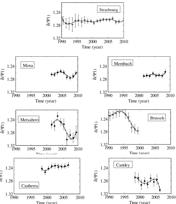
1990 1995 2000 2005 2010 1.24 1.28 1.32 Time (year) δ(Ψ 1 ) Strasbourg 1990 1995 2000 2005 2010 1.24 1.28 1.32 Time (year) δ (Ψ 1 ) Moxa 1990 1995 2000 2005 2010 1.24 1.28 1.32 Time (year) δ (Ψ 1 ) Membach 1990 1995 2000 2005 2010 1.24 1.28 1.32 Time (year) δ (Ψ 1 ) Metsahovi 1990 1995 2000 2005 2010 1.24 1.28 1.32 Time (year) δ (Ψ 1 ) Brussels 1990 1995 2000 2005 2010 1.24 1.28 1.32 Time (year) δ (Ψ 1 ) Canberra 1990 1995 2000 2005 2010 1.24 1.28 1.32 Time (year) δ (Ψ 1 ) Cantley
Figure 4. Time fluctuations of Ψ1 amplitude factor at Strasbourg, Moxa, Membach, Metsahovi, Brussels, Canberra, and Cantley SG stations obtained from ETERNA tidal analyses of 3-year running intervals shifted by 1 year. The ocean loading effect was removed using FES2004 model.
Please note that the vertical axis has been reversed.
To verify the reliability of the observed fluctuation, we analyze the data from the other 6
stations presented in Table 1. The resulting time fluctuations of δ(ψ1) obtained with 3-year running
intervals are also depicted in Fig. 4. We have also reversed the vertical axis for the sake of
comparison with Fig. 3. In agreement with the above discussion, the time variations of δ(ψ1) reflect similar changes in the resulting FCN period. The observations at other stations are not as long as those at Strasbourg station, so we can only do the comparison in a shorter common period. The data
in Brussels can be compared with the first part of the Strasbourg data from 1987 to 2000. The results we obtained for Brussels are in agreement with the time fluctuations observed by Xu and Sun (2009) with smaller error bars as we have used longer time windows. The variation amplitude of
δ(ψ1) is very large, but the decreasing and increasing period is similar compared to Strasbourg station.
The determination of tidal waves could be influenced by the position, the observation environment
of stations, the instrument state and so on, which possibly lead to a different behavior for same tidal
wave in different stations. Some variability may occur due to ocean tides effects, particularly at Brussels
and Membach that are closer to the sea than other European sites considered here. The data from Moxa,
Membach, and Metsahovi SG stations cover the period from 2001 to 2009 and can be compared with
among the results at Strasbourg, Moxa and Membach. Some values in Membach deviate from the main trend, so that the similarity is not that obvious. The situation in Metsahovi station resembles the one at Brussels site in which the amplitude variation is large but the fluctuation period matches the results obtained at Strasbourg. The last two plots are the results obtained at Canberra and Cantley stations, which are located on different continents. The available data length of these two stations was relatively short; therefore, the fluctuation is only partly displayed. The variation at Cantley station is quite different. This site is known to be well-influenced by oceanic effects. For instance the oceanic noise is larger in winter (see e.g. Rosat and Hinderer 2011). As our ocean loading correction does not include any time variability, we cannot discard the hypothesis that the apparent time variation of the delta-factors is influenced by the oceans. For Canberra station, there is
also a roughly similar variation as that in Strasbourg station. All the tests show some fluctuations in
the Ψ1 amplitude factors and also in the FCN period to a certain extent.
In the next part we will consider independent and global estimates of the FCN period using VLBI nutation observations.
4. Temporal variations of the FCN period in VLBI data
The estimate of the FCN resonance parameters using VLBI observation is known to be more precise (see for instance Rosat and Lambert, 2009). Besides, the nutation solution is obtained globally and hence minimizes the local effects that perturb VLBI antenna, such as the ones that affect the SG sites (local hydrology, oceanic noise …).
As with the SG observations, we use 6-year running intervals to estimate the transfer function values for the nutation terms section by section. We use a method similar to Vondrak et al. (2005).
The bias, trend, and two long-period terms (with arguments and 2 ) are first removed from the data sections by using the values fitted from the whole data length. We then use the least-square method to fit the selected dominant nutation terms. For the determination of the FCN parameters with VLBI data based on LSQ and Bayesian approaches, we use only the five main nutation terms mentioned in Section 2.2. Other terms have negligible effect on the results as they are much less
affected by the resonance. The observed FCN mode with a 460 day retrograde period is also fitted
simultaneously. This mode corresponds to the forced oscillation by the atmospheric and oceanic layers. In figure 5 we have plotted the fitted FCN amplitudes from VLBI observations and the corresponding values calculated with an FCN model routine “FCNNUT” of the International Earth Rotation Service (IERS Conventions, 2010). The fitted FCN amplitudes are roughly consistent with the values calculated with the FCN empirical model (this model used a –430.21 day period for the
FCN). We then use the LSQ and Bayesian methods to estimate the FCN resonance period. The results are depicted in Fig. 6(a). A very good agreement exists between the periods obtained with the two methods with only a slight difference. The error bars obtained with the Bayesian method are larger. Unlike the results obtained from SG observations, the variations of the FCN period obtained with the VLBI data are within 1 day between 1990 and 1995 but within half a day later on. Lambert
and Dehant (2007) have compared several VLBI solutions and obtained also a resonant period stable
within half a day. Besides, they have shown that the analysis strategy has also an impact of about half
19900 1995 2000 2005 2010 0.1 0.2 0.3 0.4 Time (year) a m p li tu d e ( m a s) Fitted FCN amplitude FCNNUT
Figure 5. FCN amplitudes (dots) fitted on 6-year segments shifted by a year of VLBI observations with a
460 day period and empirical FCN amplitudes with a 430.21 day period (stars) calculated with the
‘FCNNUT’ routine (IERS Conventions, 2010)
We also compare the variation between the FCN resonant period and the observed transfer function values for the retrograde annual nutation. The results show a strong inverse correlation between the FCN period and the retrograde annual nutation term. The real part values of the transfer function for this term are listed in Fig. 6(b) with the direct-axis reversed. We clearly observe also an
about 10year fluctuation in the two figures.
The nutation observation is also perturbed by global mass redistribution through angular momentum exchanges. Indeed it is worth to note that atmospheric and oceanic contributions play an important part in the observed celestial pole offsets and for the retrieval of nutation amplitudes. To remove this part, our above results include a correction for the S1 thermal atmospheric tide and other Sun-synchronous effects given in Mathews et al.(2002) for the prograde annual nutation. As the computed effects on the retrograde annual nutation varied wildly when using different atmospheric angular momentum data, Mathews et al (2002) chose to apply this correction only to the prograde annual term with amplitude about 100 as. For a better correction of the ocean and atmospheric contributions, here we also numerically integrate the Brzezinski broad-band Liouville
1990 1995 2000 2005 2010 428 429 430 431 432 Time (Year) P e ri o d ( S D ) LSQ-Sun-synchr Bayesian-Sun-synchr
equations (Brzezinski 1994; Brzezinski et al. 2002) to obtain the integrated celestial pole offsets by using atmospheric angular momentum functions (AAMF) and oceanic angular momentum functions (OAMF) data. The detailed numerical process is same as in Vondrak and Ron (2009, 2010) and will not be repetitive described here. The AAMF and OAMF we used here were computed from: (1) NCEP/NCAR re-analysis 1987-2011 (Salstein, 2005); (2) ERA+OMCT 1989-2010 (Dobslaw et al., 2010). We only use the AAMF data in (1) because the OAMF offered by ECCO model (Stammer et al. 2002; Gross et al. 2005) have not that long period. Removing the integrated celestial pole offsets, we derived the FCN resonance period with the LSQ method again and the results are depicted in Fig. 6(c). Compared to Fig. 6(a), the results obtained after correcting for the NCEP/NCAR AAMF are systematically larger, but the variation trend is similar. This is even more obvious in Fig.11 of Vondrak and Ron (2010) in which they used NCEP+ECCO data. The fluctuation of the FCN period after correction of the ERA+OMCT angular momentum functions varies more violently, as seen also in Vondrak and Ron (2010). We can also see a 10year variation trend but different than in Fig.6 (a).
1990 1995 2000 2005 2010 1.32 1.325 1.33 1.335 Time(year) -365.26 1990 1995 2000 2005 2010 428 429 430 431 432 Time (year) P e ri o d ( S D ) LSQ-NCEP LSQ-ERA+OMCT (b) (c)
Figure 6. Time variations of (a) FCN resonant period inverted from VLBI nutation data after applying
the Sun-synchronous correction of Mathews et al. (2002) ; (b) amplitude of the transfer function values
for retrograde annual nutation estimated from VLBI residuals; (c) FCN resonant period inverted from
VLBI nutation data after correction of the AAMF and OAMF contributions from either NCEP or
ERA+OMCT data. The LSQ inversion was performed on 6-year segments shifted by a year.
5. Discussion
We have investigated the time variation of the diurnal tides and FCN resonance period from SG and VLBI data. A similar decadal fluctuation in FCN period has been found in the longest SG datasets from Strasbourg station and VLBI data. Compared with the other 6 SG stations, some of them show a roughly similar variation for δ(ψ1), which make the observed fluctuation reliable in
certain extent. However, the results for δ(ψ1) at some sites are quite different no matter in amplitude or variation behavior. Thus we cannot jump to any final conclusion concerning this fluctuation. Some time variability in the oceanic effects should be checked.
The estimation of FCN period depends on the determination accuracy of related diurnal tides. Stacking global SG data (Rosat et al., 2009) could give more reliable FCN parameter in agreement with VLBI results. However to study the long time behavior, we are currently limited by the poor number of available long SG records. Besides, the present results have showed that using either a LSQ or a Bayesian method does not influence the obtained values for the FCN period.
To further verify our study, an improvement in the modeling of ocean tide loading is necessary (Ducarme et al., 2007; Rosat and Lambert, 2009), but this mainly depends on the development of more accurate ocean tidal modeling.
Considering that the ψ1 wave and the retrograde annual nutation are the closest to FCN frequency, respectively in the diurnal tidal band and the annual nutation band, the strong inverse correlation between these two terms and the FCN resonant period is reasonable
Such fluctuations in the tidal amplitude factors were already mentioned by Lecolazet (1983),
who indicated some correlations between the variations of some tidal amplitude factors (P1, K1, Ψ1, Ф1, and M2) and the length of day (LOD) variations. In our study, such correlation does not appear.
Only K1 and Ψ1 amplitude factors have relatively similar variations. To check for a possible correlation with LOD, we plot the variations of LOD data offered by IERS EOP observations in Fig. 7 (finals2000A.all). The relative amplitude factors of Ψ1, K1, and M2 are also plotted in Fig.7. We
can see that there is no clear correlation between the tidal waves and LOD fluctuations.
are mainly explained by the core mantle coupling. According to the spectral analysis of the LOD
data, the main power of the spectrum is at the decade scale, in which the main peak is a component of period about 22 years. Besides, there are also some seasonal and interannual signal components. In
order to check whether such a consistent fluctuation in LOD exists, other signal components should
be eliminated. First, we use a Butterworth low-pass filter to remove the large components with periods of less than 1 year. We then use a LSQ method (Guo & Han, 2009) to fit the 22-year term and other interannual signals. After these terms are deducted from LOD data, the residuals are plotted in Fig. 7 (continuous red line). The 10-year oscillation is clearly visible. The fluctuation we
have found in the FCN period is also about 10 years. Compared with the FCN results of previous
figures, there is about a 2 year phase difference between the variations of LOD and FCN period. It is
important to point out that more detailed work is needed to process the LOD data and separate the
decade scale signal, as well as to explain the phase difference. However, the decade variations in LOD and its relation with core mantle couplings may be helpful to explain some fluctuations in the FCN period. Vondrak and Ron (2010) have also concluded indeed that the observed variations could be real and due to some processes at the CMB, as the current AAMF and OAMF modeling cannot explain the observed variations of the FCN period.
As mentioned in Section 1, the period of the FCN strongly depends on the structure and physical properties at CMB (e.g., Koot et al., 2010). Indeed, the frequency of the FCN depends on
coupling mechanisms at the core boundaries (Greff-Lefftz and Legros, 1999; Mathews et al., 2002).
In a celestial reference frame, it can be written (normalization by ):
Ω
−
+
Ω
+
+
+
+
+
−
+
−
−
=
²
2
²
2
1
1
20 f P p f p p f s ICB CMB f m f FCNA
A
D
i
A
C
B
f
A
A
K
K
e
A
A
β
β
σ
, (7)-1 0 1 2 3 ∆L O D ( m s) ∆LOD Residual Polynomial fitting 1.09 1.1 1.11 0.9834 0.9836 1990 1995 2000 2005 2010 1.0074 1.0078 Time (year) δ(Ψ1)/δ(O1) δ(K1)/δ(O1) δ(M 2)/δ(O1)
where ef is the dynamic ellipticity of the outer core; As, Af, and Am are respectively the mean
principal moments of inertia of the solid inner core, the fluid outer core, and the mantle. Kcmb and
Kicb are the complex coupling strength parameters representing the influence of the electromagnetic torques at CMB and ICB, respectively; Ap, Bp, Cp, and Dp are the coefficients of the torque due to the driven geostrophic pressure acting on the topography at CMB (Greff-Lefftz and Legros, 1999);
0 2
f is the ratio of the geostrophic pressure at the CMB over the hydrostatic rotational pressure and β is a compliance that characterizes the deformability of the CMB under the centrifugal force.
2 / 1 0 f h q =
β
, where h1f is the Love number expressing the deformation of the CMB under aninertial pressure (Dehant et al., 1993). Besides, a misalignment (tilt) of the inner core with respect to
the mantle could also influence the direction of the Earth’s rotation on decade timescale (Dumberry
and Bloxham, 2002) and slightly perturb the FCN frequency through gravitational and pressure torque. Such an expression shows that the eigenfrequency of the FCN could vary when the torques
vary. Impact of time-varying torques on the FCN period has not been computed yet and would
Figure 7. Variations of LOD, residuals after removing the 22-year and inter-annual terms,
and relative amplitude factors of K1, Ψ1, and M2 obtained from 6-year segments shifted by a year
of Strasbourg SG data (the vertical axis is not reversed in this figure)
6. Conclusion
According to our study, the variations in time of the FCN resonance period are within 1 day from VLBI data and within several days from SG records.
Considering the error bars, the variations of the FCN period are however not obvious.
We have shown a similar variation trend in the results obtained from different worldwide SG data. There exists also a similar trend in the FCN period obtained from VLBI observations as previously observed by Vondrak and Ron (2010). The test of using two kinds of independent observation (surface gravity on the one hand and VLBI nutation on the other hand) to verity the time variability of the FCN period seems coherent. However longer records at more SG sites would be necessary to confirm such fluctuations. For SG data, improvement of ocean tidal loading correction should be considered in a future study. For celestial pole offsets, further studies are required to reach agreement between the different models of atmospheric and oceanic angular momentum functions. The variation trend of the FCN period totally depends on the retrograde annual term in nutation and on the Ψ1 wave in tidal gravity. It is indeed the same phenomenon in different reference frames,and the decadal fluctuation seems to exist in both datasets. However the processes responsible for such variation are not clearly identified yet. A time-variability in the ocean loading and angular momentum is one candidate as well as some varying torques at the CMB. A possible
correlation with the decadal LOD trend due to some core-mantle coupling mechanism may exist, but no clear evidence or demonstration has been proposed yet. Further theoretical computations are needed to demonstrate a possible time fluctuation in the FCN period of geophysical origin.
Acknowledgments
This work was supported by the Major State Basic Research Development Program of China (2014CB845902), National Natural Science Foundation of China (41321063, 41274085 and 41304058). We are very thankful to the Global Geodynamics Project and the International VLBI Service for Geodesy and Astrometry for providing SG and VLBI data. We would like to thank two anonymous reviewers for their comments to improve the manuscript.
References
Amoruso, A., Botta, V. and L. Crescentini, 2012. Free Core Resonance parameters from strain data: sensitivity analysis and results from the Gran Sasso (Italy) extensometers, Geophys. J. Int., 189, 923–936.
Brzeziński, A.: 1994, Polar motion excitation by variations of the effective angular momentum function: II. Extended model. Manuscripta Geodaetica. 19, 157–171.
Brzeziński, A., Bizouard, C., and Petrov, S.: 2002, Influence of the atmosphere on Earth rotation: What can be learned from the recent atmospheric angular momentum estimates? Surveys in Geophysics 23, 33–69.
Buffett, B.A., 1996. A mechanism for decade fluctuations in the length of day, Geophys. Res. Lett., 23, 3803–3806.
Buffet, B.A., Mound, J., Jackson, A., 2009. Inversion of torsional oscillations for the structure and dynamics of Earth’s core, Geophys. J. Int., 177, 878-890.
Defraigne P, Dehant V, Hinderer J., 1994. Stacking gravity tides measurements and nutation observations in order to determine the complex eigenfrequency of nearly diurnal free wobble. J Geophys Res, 99: 9203―9213.
Dehant, V., Hinderer, J., Legros, H., Lefftz, M., 1993. Analytical approach to the computation of the Earth, the outer core and the inner core rotational motions. Phys. Earth Planet. Inter. 76, 259–282.
Dobslaw, H., R. Dill, A. Groetzsch, A. Brzezinski, and M. Thomas, 2010. Seasonal polar motion excitation from numerical models of atmosphere, ocean, and continental hydrosphere, J. Geophys. Res., 115, B10406, doi:10.1029/2009JB007127.
Ducarme, B., Sun, H.-P., Xu, J.-Q., 2007. Determination of the free core nutation period from tidal gravity observations of theGGPsuperconducting gravimeter network. J. Geod. 81, 179–187. Dumberry, M., Bloxham, J., 2002. Inner core tilt and polar motion, Geophys. J. Int., 151, 377-392. Farrell, W. E. (1972). Deformation of the Earth by surface load. Rev. Geoph., 10,761-779.
Florsch N, Hinderer J. Bayesian estimation of the free core nutation parameters from the analysis of precise tidal gravity data. Phys Earth Planet Inter, 2000, 117: 21–35
Greff-Lefftz, M., Legros, H., 1999. Magnetic field and rotational eigenfrequencies, Phys. Earth Planet. Int., 112, 21-41.
Gross, R. S., Fukumori, I., and Menemenlis, D.: 2005, Atmospheric and oceanic excitation of decadal-scale Earth orientation variations, J. Geophys. Res., 110, B09405, doi:10.1029/2004JB003565.
Guo J.Y., Han, Y. B., 2009. Seasonal and inter-annual variations of length of day and polar motion observed by SLR in 1993―2006. Chinese Science Bulletin, 54(1): 46-52
Hartmann T, Wenzel H G. The HW95 tidal potential catalogue. Geophysical Research Letters, 1995, 22: 3553–3556.
Hinderer, J., Legros, H. and Crossley, D. J. Global earth dynamics and induced gravity changes, J. Geophys. Res,1991, 96: 20257-20265.
Hinderer J, Boy J P, Gegout P, et al. 2000. Are the free core nutation parameters variable in time? Phys Earth Planet Inter, 117: 37―49.
Holme, R., 1998. Electromagnetic core–mantle coupling—I. Explaining decadal changes in the length of day, Geophys. J. Int., 132, 167-180.
IERS Conventions (2010). Gérard Petit and Brian Luzum (eds.). (IERS Technical Note ; 36) Frankfurt am Main: Verlag des Bundesamts für Kartographie und Geodäsie, 2010. 179 pp., ISBN 3-89888-989-6
Koot, L. , Dumberry, M., Rivoldini, A., de Viron, O. and Dehant, V., 2010. Constraints on the coupling at the core–mantle and inner core boundaries inferred from nutation observations, Geophys. J. Int., 182, 1279-1294.
Lambert S. B., Dehant, V., 2007. The Earth’s core parameters as seen by the VLBI, Astron. Astrophys., 469, 777-781.
Lecolazet, R., 1983. Correlation between diurnal gravity tides and the Earth’s rotation rate, in Proc. 9th Int. Symp. Earth Tides, pp. 527-530, ed. Kuo J.T., Schweizerbart, Stuttgart.
Liu Ming-bo Sun He-ping Xu Jian-qiao Zhou Jiang-cun, 2007.Determination of the Earth’s Free Core Nutation Parameters by Using Tidal Gravity Data, Acta Seismologica Sinica, 20, 6
708-711.
Lyard, F., Lefevre, F., Letellier, T., Francis, O., 2006. Modelling the global ocean tides: modern insights from FES2004. Ocean Dynam. 56, 394–415.
Marquardt, D., 1963. An algorithm for least-squares estimation of non-linear parameters. J. Soc. Ind. Appl. Math. 11 (2), 431–441.
Mathews P M, Herring T A, Buffett B A, 2002. Modeling of nutation and precession: New nutation series for nonrigid Earth and insights into the Earth’s interior. J Geophys Res, 2002, 107: 539—554
Melchior P., Moens M., Ducarme B., 1980. Computations of tidal gravity loading and
attraction effects. Bull. Obs. Marées Terrestres, Obs. Royal Belg., 4, 5, 95-133
Roosbeek F, Defraigne P., Fessel, M., Dehant, V., 1999. The free core nutation period stays between 431 and 434 sidereal days. Geophysical Research Letters, 26: 131―134
Rosat, S. & Lambert, S.B., 2009. Free core nutation resonance parameters from VLBI and superconducting gravimeter data, Astron. Astrophys., 503, 287-291.
Rosat S. and J. Hinderer, 2011. Noise Levels of Superconducting Gravimeters: Updated Comparison and Time Stability, Bull. Seism. Soc. Am., vol. 101, no. 3, June 2011, doi:10.1785/0120100217.
Rosat, S., Florsch, N., Hinderer, J., Llubes, M., 2009. Estimation of the Free Core Nutation parameters from SG data: sensitivity study and comparative analysis using linearized Least-Squares and Bayesian methods, J. of Geodyn., 48: 331–339
Salstein, D., 2005. Computing atmospheric excitation functions for Earth rotation/polar motion. Cahiers du Centre Européen de Géodynamique et de Séismologie 24, Luxembourg, 83–88.
Sun, H., Jentzsch, G., Xu J. et.al. 2004. Earth’s free core nutation determined using C032 superconducting gravimeter at station Wuhan/China. J Geodyn, 38:451–460.
Tarantola, A., Valette, B., 1982a. Inverse problems = quest for information. J. Geophys, , 50: 159–170.
Tarantola, A., Valette, B., 1982b. Generalized nonlinear inverse problems solved using the least squares criterion. Rev. Geophys. Space Phys. 20 (2), 219–232.
Vondrak J, Weber R, Ron C., 2005. Free core nutation: direct observations and resonance effects. Astr. Astrophys., 444:297―303
Vondrak J, Ron C., 2009. Stability of period and quality factor of free core nutation. Acta Geodyn Geomater., Vol. 6, No. 3 (155), 217–224
Vondrak J, Ron C., 2010. Study of atmospheric and oceanic excitations in the motion of Earth’s spin axis in space. Acta Geodyn Geomater., Vol. 7, No. 1 (157), 19–28
Xu, J. and H. Sun. 2009. Temporal variations in free core nutation period. Earthq Sci, 22: 331―336 Wallace, P. T., Capitaine, N., 2006. Precession-nutation procedures consistent with IAU 2006
resolutions, Astron. Astrophys., 459, 981-985.
Wenzel, H.-G., 1996. The nanogal software: earth tide data processing package ETERNA 3.30. Bull. Inf. Marées Terrestres 124, 9425–9439.