HAL Id: hal-00681203
https://hal.archives-ouvertes.fr/hal-00681203
Submitted on 20 Mar 2012HAL is a multi-disciplinary open access archive for the deposit and dissemination of sci-entific research documents, whether they are pub-lished or not. The documents may come from
L’archive ouverte pluridisciplinaire HAL, est destinée au dépôt et à la diffusion de documents scientifiques de niveau recherche, publiés ou non, émanant des établissements d’enseignement et de
A Logic of Reachable Patterns in Linked
Data-Structures
Greta Yorsh, Alexander Rabinovich, Mooly Sagiv, Antoine Meyer, Ahmed
Bouajjani
To cite this version:
Greta Yorsh, Alexander Rabinovich, Mooly Sagiv, Antoine Meyer, Ahmed Bouajjani. A Logic of Reachable Patterns in Linked Data-Structures. Journal of Logic and Algebraic Programming, Elsevier, 2007, 73 (1-2), p. 111-142. �10.1016/j.jlap.2006.12.001�. �hal-00681203�
A Logic of Reachable Patterns
in Linked Data-Structures
Greta Yorsh
a,∗
,1Alexander Rabinovich
aMooly Sagiv
aAntoine Meyer
bAhmed Bouajjani
baSchool of Computer Science, Tel-Aviv University, Tel-Aviv, Israel.
Email addresses: gretay,rabinoa,[email protected]
bLIAFA laboratory, University of Paris 7, Paris, France.
Email addresses: ameyer,[email protected]
Abstract
We define a new decidable logic for expressing and checking invariants of programs that manipulate dynamically-allocated objects via pointers and destructive pointer updates. The main feature of this logic is the ability to limit the neighborhood of a node that is reachable via a regular expression from a designated node. The logic is closed under boolean opera-tions (entailment, negation) and has a finite model property. The key technical result is the proof of decidability.
We show how to express precondition, postconditions, and loop invariants for some in-teresting programs. It is also possible to express properties such as disjointness of data-structures, and low-level heap mutations. Moreover, our logic can express properties of arbitrary data-structures and of an arbitrary number of pointer fields. The latter provides a way to naturally specify postconditions that relate the fields on procedure’s entry to the field on procedure’s exit. Therefore, it is possible to use the logic to automatically prove partial correctness of programs performing low-level heap mutations.
Key words: Program Verification, Shape Analysis, Heap-manipulating programs,
Decidable logic with reachability, Reachability, Routing expression, Pattern, Transitive closure logics, Weak monadic second-order logic
1991 MSC: 03B25, 11U05, 03B45, 03B15, 68N15, 68N30, 68N19
∗ Corresponding author
1 This research was supported by THE ISRAEL SCIENCE FOUNDATION (grant No 304/03).
1 Introduction
The automatic verification of programs with dynamic memory allocation and pointer manipulation is a challenging problem. In fact, due to dynamic memory allocation and destructive updates of pointer-valued fields, the program memory can be of ar-bitrary size and structure. This requires the ability to reason about a potentially in-finite number of memory (graph) structures, even for programming languages that have good capabilities for data abstraction. Usually abstract-datatype operations are implemented using loops, procedure calls, and sequences of low-level pointer manipulations; consequently, it is hard to prove that a data-structure invariant is reestablished once a sequence of operations is finished [27].
To tackle the verification problem of such complex programs, several approaches emerged in the last few years with different expressive powers and levels of au-tomation, including works based on abstract interpretation [35,46,42], logic-based reasoning [31,43], and automata-based techniques [32,37,8]. An important issue is the definition of a formalism that (1) allows us to express relevant properties (invariants) of various kinds of linked data-structures, and (2) has the closure and decidability features needed for automated verification. The aim of this paper is to study such a formalism based on logics over arbitrary graph structures, and to find a balance between expressiveness, decidability and complexity.
Reachability is a crucial notion for reasoning about linked data-structures. For in-stance, to establish that a memory configuration contains no garbage elements, we must show that every element is reachable from some program variable. Other ex-amples of properties that involve reachability are (1) data-structure invariants, e.g., the tail of a queue is reachable from the head of a queue, (2) the acyclicity of data-structure fragments, i.e., every element reachable from node u cannot reach u, (3) the property that a data-structure traversal terminates, e.g., there is a path from a node to a sink-node of the data-structure, (4) the property that, for programs with procedure calls when references are passed as arguments, elements that are not reachable from a formal parameter are not modified.
A natural formalism to specify properties involving reachability is the first-order logic over graph structures with transitive closure. Unfortunately, even simple de-cidable fragments of first-order logic become undede-cidable when transitive closure is added [21,29].
In this paper, we propose a logic that can be seen as a fragment of the first-order logic with transitive closure. Our logic (1) is simple and natural to use, (2) is ex-pressive enough to cover important properties of a wide class of arbitrary linked data-structures, and (3) allows for algorithmic modular verification using program-mer’s specified loop-invariants and procedure’s specifications.
proposi-tions (called reachability constraints) modelling reachability between heap objects pointed-to by program variables and other heap objects with certain properties. The properties are specified using patterns that limit the neighborhood of an object.
For example, we can specify the property that an objectv is an element of a doubly-linked list using a the pattern invf,b, defined by (v→w) ⇒ (wf →v). This patternb
says that ifv has an emanatingforwardpointerf that leads to an object w, then w has a backward pointer b into v. Using the pattern invf,b, we can describe a
doubly-linked list pointed-to by a program variable x by the atomic proposition x[f
→∗]invf,bin our logic. This reachability constraint says that any objectv
reach-able from an object pointed-to byx using a (possibly empty) sequence offorward
pointers satisfies the propertyinvf,b. 2
The design of our logic is guided by the following principles. First, reachability constraints are closed formulas without quantifier alternations. This guarantees that we are dealing with alternation-free formulas. Second, reachability is expressed via Kleene star operator. We believe that regular expressions is a more natural notation than transitive closure operator. Third, decidability is obtained by syntactically re-stricting the way patterns are formed. In particular, the use of equality is limited. Semantically, the restriction means that a pattern cannot relate between two nodes that are distant from one another, unless the nodes are “named”. As a result, a pat-tern can only describe local properties. Global properties can only be described using reachability along regular paths that start from “named” nodes. Therefore, complex properties can be enforced only between “named” nodes. For example, complex sharing patterns can be created around objects pointed-to by program vari-ables; arbitrary sharing is allowed but cannot be enforced deep in the data-structure, because the objects that are deep are indistinguishable and distant nodes cannot be related by a pattern.
The contributions of this paper can be summarized as follows:
• We define the logic L0where reachability constraints such as those mentioned
above can be used. Patterns in such constraints are defined by quantifier-free first-order formulas over graph structures and sets of access paths are defined by regular expressions.
• We show that L0 has a finite-model property, i.e., every satisfiable formula
has a finite model. Therefore, invalid formulas are always falsified by a finite store.
• We prove that the logic L0 is, unfortunately, undecidable.
• We define a suitable restriction on the patterns leading to a fragment of L0
calledL1.
• We prove that the satisfiability (and validity) problem is decidable. The frag-mentL1 is the main technical result of the paper and the decidability proof is
non-trivial. The main idea is to show that every satisfiableL1 formula is also
satisfied by a tree-like graph. Thus, even though L1 expresses properties of
arbitrary data-structures, because the logic is limited enough, a formula that is satisfied on an arbitrary graph is also satisfied on a tree-like graph. There-fore, it is possible to answer satisfiability (and validity) queries forL1using a
decision procedure for weak monadic second-order logic (MSO) on trees. • We show that despite the restriction on patterns we introduce, the logic L1
is still expressive enough for use in program verification: various important data-structures, and loop invariants concerning their manipulation, are in fact definable inL1.
• We show that the proof of decidability of L1 holds “as is” for many useful
extensions ofL1.
We define Logic of Reachable Patterns (LRP for short) to be one of the decid-able extension ofL1 (see Section 9 for details). The new logic LRP forms a basis
of the verification framework for programs with pointer manipulation, which is a subject of an ongoing work. For instance, in contrast to decidable logics that re-strict the graphs of interest (such as weak monadic second-order logic on trees), our logic allows arbitrary graphs with an arbitrary number of fields. We show that this is very useful even for verifying programs that manipulate singly-linked lists in order to express postcondition and loop invariants that relate the input and the output state. By restricting the syntax, we guarantee that queries posed over arbi-trary graphs can be answered by considering only tree-like graphs. This approach allows us to automate the reasoning about limited but interesting properties of ar-bitrary graphs. Moreover, our logic strictly generalizes the decidable logic in [4], which inspired our work. Therefore, it can be shown that certain heap abstractions including [24,45] can be expressed using LRP formulas.
The rest of the paper is organized as follows: Section 2 defines the syntax and the semantics ofL0, and shows that it has a finite model property; Section 3 shows that
L0 is undecidable; Section 4 defines the fragmentL1, demonstrates the
expressive-ness ofL1 on several examples, and defines an interesting extension ofL1, called
L2; Section 5 presents the decidability proof for L1, with a detailed proof of the
main theorem given in Section 6; Section 7 sketches the proof of decidability of L2, which does not immediately follow from the one ofL1; Section 8 contains the
complexity results forL1; Section 9 discusses the limitations and the extensions of
the new logics; finally, Section 10 discusses the related work.
2 TheL0Logic
In this section, we define the syntax and the semantics of our logic. For simplicity, we explain the material in terms of expressing properties of heaps. However, our logic can actually model properties of arbitrary directed graphs. Still, the logic is
powerful enough to express the property that a graph denotes a heap.
2.1 Syntax ofL0
L0 is a propositional logic over reachability constraints. That is, anL0formula is a
boolean combination of closed formulas in first-order logic with transitive closure that satisfy certain syntactic restrictions.
Letτ = hC, U, F i denote a vocabulary, where
• C is a finite set of constant symbols usually denoting designated objects in the heap, pointed to by program variables;
• U is a set of unary relation symbols denoting properties, e.g., color of a node in a Red-Black tree;
• F is a finite set of binary relation symbols (edges) usually denoting pointer fields.3
For example, we can describe a doubly-linked list with forward pointer f and backward pointer b, pointed-to by a program variable x, using the vocabulary in which C = {x}, U = {}, and F = {f, b}. We can describe a Red-Black tree pointed-to by a program variableroot using the vocabulary in which C = {root}, U = {red, black}, and F = {right, lef t}.
A termt is either a variable or a constant. An atomic formula is an equality t = t′,
a monadic formula u(t) for some u ∈ U , or an edge formula tf
→t′ for some f ∈ F , and terms t, t′. A quantifier-free formula ψ(v
0, . . . , vn) over τ and variables
v0, . . . , vn is an arbitrary boolean combination of atomic formulas. We say that
a sub-formula ψ appears positively (negatively) in ϕ, if ψ appears under an even (odd) number of negations inϕ. Let F V (ψ) denote the free variables of the formula ψ.
Definition 2.1 A neighborhood formula N (v0, . . . , vn) is a conjunction of edge
formulas of the formv f
→v′, wheref ∈ F and v, v′ ∈ {v0, . . . , vn}, and monadic
formulas of the formu(v) or ¬u(v), where u ∈ U .
Definition 2.2 LetN (v0, . . . , vn) be a neighborhood formula. The Gaifman graph
ofN , denoted by BN, is an undirected graph with a vertex for each free variable
of N . There is an edge between the vertices corresponding to vi and vj inBN if
and only if(vi→vf j) appears in N , for some f ∈ F . The distance between logical
variables vi and vj in the formula N is the minimal edge distance between the
corresponding verticesvi andvj inBN.
For example, for the formulaN = (v0→vf 1) ∧ (v0→vf 2) the distance between v1and
v2 inN is 2, and its underlying graph BN looks like this:v1—v0 —v2.
Definition 2.3 A routing expression is an extended regular expression, defined as
follows:
R ::= ∅ empty set
| ǫ empty path
| f
→ f ∈ F forward along edge | f
← f ∈ F backward along edge | u u∈ U test if u holds
| ¬u u∈ U test if u does not hold | c c∈ C test if c holds
| ¬c c∈ C test if c does not hold | R1.R2 concatenation
| R1|R2 union
| R∗ Kleene star
Intuitively, a routing expression describes a path in the heap.
A routing expression can require that a path traverse some pointer fields backwards. For example, the routing expression f
→∗.←f ∗ describes a sequence off -edges that may look like this: f
→→f ←f ←f ←. We use this routing expression in Section 4.2 tof describe disjoint data-structures.
A routing expression has the ability to test properties of heap objects along the path. For example, a routing expression(f
→.¬y)∗ describes a path which does not traverse an object pointed-to by the program variabley. We use this routing expres-sion to describe a path along which some property holds until the path reaches the object pointed-to byy (see Section 4.2).
Definition 2.4 (Syntax ofL0) A reachability constraint is a closed formula of the
form:
∀v0, . . . , vn.R(c, v0) ⇒ (N (v0, . . . , vn) ⇒ ψ(v0, . . . , vn)) (1)
wherec ∈ C is a constant, R is a routing expression, N is a neighborhood formula, andψ is an arbitrary quantifier-free formula, such that F V (N ) ⊆ {v0, . . . , vn} and
F V (ψ) ⊆ F V (N ) ∪ {v0}. In particular, if the neighborhood formula N is true
(the empty conjunction), thenψ is a formula with a single free variable v0.
AnL0formula is a boolean combination of reachability constraints.
p(v0). Here, the designated variable v0denotes the “central” node of the
“neighbor-hood” reachable fromc by following an R-path. Intuitively, neighborhood formula N binds the variables v0, . . . , vnto nodes that form a subgraph, andψ defines more
constraints on those nodes. 4
For example, the pattern detf(v0) defined by the formula (v0→vf 1) ∧ (v0→vf 2) ⇒
(v1 = v2) ensures that v0 has at most one outgoing f -edge. The neighborhood
formula(v0→vf 1)∧(v0→vf 2) contains two edges emanating from the central node v0.
The restriction on the neighborhood is that the edges are in fact the same, because they have the same source,v0, the same target,v1 = v2, and the same labelf .
We use let expressions to specify the scope in which the pattern is declared:
letp1(v0) def
= N1(v0, . . . , vn) ⇒ ψ1(v0, . . . , vn) in ϕ
This allows us to write more concise formulas via reuse of pattern definitions. For example, we can say that program variables x and y are pointing to (potentially shared) doubly-linked lists:
letinvf,b(v0) def
= (v0→vf 1 ⇒ v1→vb 0) in x[→]invf f,b∧ x[→]invf f,b
2.1.1 Shorthands
We use c[R]p to denote a reachability constraint (1). Intuitively, the reachability constraint requires that every node that is reachable fromc by following an R-path satisfy the patternp.
We use c1[R]¬c2 to denote letp(v0) def
= (true ⇒ ¬(v0 = c2)) in c1[R]p. In this
simple case, the neighborhood is only the node assigned tov0. Intuitively,c1[R]¬c2
means that the node labeled by constantc2 is not reachable along anR-path from
the node labeled byc1. We usec1hRic2 as a shorthand for¬(c1[R]¬c2). Intuitively,
c1hRic2 means that there exists anR-path from c1 toc2. We usec1 = c2 to denote
c1hǫic2, andc1 6= c2 to denote¬(c1 = c2).
We usec[R](p1 ∧ p2) to denote (c[R]p1) ∧ (c[R]p2), when p1 andp2 agree on the
central node variable. When two patterns are often used together, we introduce a name for their conjunction (instead of naming each one separately): let p(v0)
def
= (N1 ⇒ ψ1) ∧ (N2 ⇒ ψ2) in ϕ.
For a quantifier-free formulaψ(v0) with a single free variable v0, we write c[R]ψ
instead of letp(v0) def
= (true ⇒ ψ(v0)) in c[R]p. If ψ(v0) has only monadic
formu-las, we omit the free variablev0 from it. In particular, for a unary relation symbol
u, we use c[R]u to denote let p(v0) def
= (true ⇒ u(v0)) in c[R]p. We use u(c) to 4 In all our examples, a neighborhood formula N used in a pattern is such that BN (the Gaifman graph ofN ) is connected.
denote the formula chǫiu (equivalently, c[ǫ]u). We abuse the notations slightly by writingN ∧ ψ1 ⇒ ψ2instead ofN ⇒ (ψ1 ⇒ ψ2).
In routing expressions, we use Σ
→ to denote the routing expression (f1
→|f2
→| . . . |fm
→), the union of all the fields inF . Similarly, Σ
← denotes the routing expression (f1
←|f2
←| . . . |fm
←). For example,c1[→Σ∗]¬c2means thatc2is not reachable fromc1by any path. Finally,
we sometimes omit the concatenation operator “.” in routing expressions.
2.2 Semantics ofL0
L0 formulas are interpreted over labeled directed graphs. A labeled directed graph
G over a vocabulary τ = hC, U, F i is a tuple hVG, EG, CG, UGi where:
• VGis a set of nodes modelling the heap objects,
• EG: F → P(VG× VG) are labeled edges,
• CG: C → VG provides interpretation of constants as unique labels on the
nodes of the graph, and
• UG: U → P(VG) maps unary relation symbols to the set of nodes in which
they hold.
The languageL(R) of words accepted by a routing expression R is defined as usual for regular expression. The semantics ofL0formulas is formally defined as follows.
Definition 2.5 Consider a routing expressionR and w ∈ L(R). We say that there
is a path labeled by w from a node s1 to a node s2 in G if one of the following
conditions holds:
• s1 = s2 andw = ǫ,
• s1 = s2,w = u for a unary relation symbol u and s1 ∈ UG(u),
• s1 = s2,w = ¬u for a unary relation symbol u and s1 ∈ U/ G(u),
• s1 = s2,w = c for a constant c and CG(c) = s1,
• s1 = s2,w = ¬c for a constant c and CG(c) 6= s1,
• w = f
→ for an edge f ∈ F and hs1, s2i ∈ EG(f ),
• w = f
← for an edge f ∈ F and hs2, s1i ∈ EG(f ),
• w = w1.w2and there exists a nodes3such that there is a path labeled byw1
froms1tos3 and there exists a path labeled byw2froms3 tos2 .
A node tuple in G satisfies a pattern p if it satisfies the quantifier-free formula that definesp, according to the usual semantics of the first-order logic over graph structures.
The satisfaction relation|= between a graph G and L0formulas is defined similarly
to the usual semantics the first-order logic with transitive closure over graphs. A graphG satisfies a formula c[R]p (and we write G |= c[R]p) if and only if for every
w ∈ L(R) and for every node tuple s0, . . . , sninG, if there is a path labeled by w
fromc to s0, then the tuples0, . . . , sn, satisfiesp with s0 used as the central node
forp. The meaning of Boolean connectives is defined in a standard way.
We say that nodes ∈ G is labeled with σ if σ ∈ C and s = CG(σ) or σ ∈ U and
s ∈ UG(σ). For an edge hs
1, s2i ∈ G and f ∈ F , we say that hs1, s2i is labeled
with f , if hs1, s2i ∈ EG(f ). In the rest of the paper, graph denotes a directed
labeled graph, in which nodes are labeled by constant and unary relation symbols, and edges are labeled by binary relation symbols, as defined above.
Remark. The translation from L0 to MSO in Section 5.1 provides an alternative
definition for the semantics ofL0.
2.3 Finite Model Property
We are interested in checking validity (and satisfiability) ofL0 formulas only over
finite graphs. The graphs are finite because they represent data-structures allocated by a program. (However, the graphs may be unbounded, due to dynamic allocation of memory.) In general, finite validity problem is considered more difficult than validity. For example, in first-order logic, validity problem is recursively enumer-able while finite validity is not. In a logic with finite model property, the notions of validity and finite validity coincide. Thus, finite model property is desirable.
L0 with arbitrary patterns has a finite model property. If formula ϕ ∈ L0 has an
infinite model, each reachability constraint inϕ that is satisfied by this model has a finite witness.
Theorem 2.6 (Finite model property) Every satisfiableL0 formula is satisfiable
by a finite graph.
Sketch of Proof: We show thatL0can be translated into a fragment of an infinitary
logic that has a finite model property. Observe thatc[R]p is equivalent to an infinite conjunction of universal first-order sentences. Therefore, ifG is a model of c[R]p then every subgraph of G is also its model. Dually, ¬c[R]p is equivalent to an infinite disjunction of existential first-order sentences. Therefore, ifG is a model of ¬c[R]p, then G has a finite subgraph G′such that every subgraph ofG that contains
G′ is a model of¬c[R]p. It follows that every satisfiable boolean combination of
Fig. 1. A sketch of a grid model for a tiling problemT . The n-edges are depicted with solid lines, the b-edges are depicted with dashed lines. The filled circles denote nodes labeled with “red”.
3 Undecidability ofL0
The satisfiability and the validity problems ofL0 formulas are undecidable. Since
L0 is closed under negation, it is sufficient to show that its satisfiability problem is
undecidable. The proof uses a reduction from the tiling problem.
Definition 3.1 Define a tiling problem,T = hT, R, Di, to consist of a finite list of tile types,T = [t0, . . . tk], together with horizontal and vertical adjacency relations,
R, D ⊆ T2. Here R(a, b) means that tiles of type b fit immediately to the right of
tiles of typea, and D(a, b) means that tiles of type b fit one step down from those of typea. A solution to a tiling problem is an arrangement of instances of the tiles in a rectangular grid such that at0 tile occurs in the top left node of the grid, and a
tk tile occurs in the bottom right node of the grid, and all adjacency relationships
are respected.
It is well-known that tiling problems of this flavor are undecidable. Therefore, if a logic can express tilings, its satisfiability problem is also undecidable. Given a tiling problemT , we construct a formula ϕT, such thatϕT is satisfiable if and only
if there exists a solution toT .
The idea is that each node in the graph that satisfiesϕT describes a tile, with unary
relation symbolsT0, . . . , Tk encoding the tile typest0, . . . tk. There is ab-edge
be-tween every two nodes that are vertically adjacent in the grid. There is ann-edge between every two nodes that are horizontally adjacent in the grid, and from the last node of every row to the first node in the subsequent row. The constantc labels the top left node of the grid, the constantc′ labels the top right node of the grid, the
constantc′′ labels the first node of the second row of the grid, and the constantc′′′
labels the bottom right node of the grid (see sketch in Fig. 1). The unary relation red labels the nodes of the last column of the grid.
The most interesting part of the formulaϕT ensures that all graphs that satisfyϕT
have a grid-like form. It states that for every nodev that is n-reachable from c, if there is ab-edge from v to u, then there is a b-edge from the n-successor of v to the
n-successor of u:
let p(v) def
= (v b
→u) ∧ (v→vn 1) ∧ (u→un 1) ⇒ (v1→ub 1) in c[(→)n ∗]p (2)
Theorem 3.2 (Undecidability) The satisfiability problem ofL0formulas is
unde-cidable.
Proof: Given a tiling problemT = hT, R, Di, we construct an L0 formulaϕT as a
conjunction of the following formulas:
(1) There isn-path from c to c′:ch(n
→)∗ic′ (2) There isn-edge from c′ toc′′:c′hn
→ic′′ (3) There isn-path from c′′ toc′′′:c′′h(n
→)∗ic′′′ (4) There isb-edge from c to c′′:ch b
→ic′′. (5) Non-edge exits t: c′′′[n
→]f alse.
(6) For every node v that is n-reachable from s, if there is a b-edge from v to u, then there is a b-edge from the n-successor of v to the n-successor of u:
letp(v) def
= (v b
→u) ∧ (v→vn 1) ∧ (u→un 1) ⇒ (v1→ub 1) in c[(→)n ∗]p.
(7) Then-edges and the b-edges reachable from s are deterministic: let detn(v) def
= (v n
→v′) ∧ (v→vn ′′) ⇒ (v′ = v′′) in s[(→)n ∗]detn, similarly, forb-edges.
(8) The top left node of the grid has a t0 tile type, and the bottom right node of
the grid has atktile type:T0(c) ∧ Tk(c′′′).
(9) Each node in the grid has exactly one tile type:
c[( n →)∗] ^ 0≤i<j≤k ¬(Ti∧ Tj) ∧ _ 0≤i≤k Ti
(10) Every node in the last column of the grid is labeled withred: c′[( b
→)∗]red. (11) To express that only nodes in the last column of the grid are labeled withred,
we say that the first row is not labeled withred, except its last node, and if a node is labeled withred, then its b-predecessor is labeled:
c[( n
→.¬c′)∗]¬red ∧ let p(v)= (wdef →v) ∧ red(v) ⇒ red(w) in c[(b →)n ∗]p (12) Two horizontally adjacent tiles are compatible according toR:
letp(v) def = (v n →w) ∧ ¬red(v) ⇒ _ R(ti,tj) (Ti(v) ∧ Tj(w)) inc[(→)n ∗]p
(13) Two vertically adjacent tiles are compatible according toD:
Remark. The reduction uses only two binary relation symbols and a fixed number
of unary relation symbols. It can be modified to show that the logic with three binary relation symbols (and no unary relations) is undecidable.
4 Decidable and Useful Fragments ofL0
In this section we define two fragments ofL0and show their usefulness. In the next
section, we show that these fragments are decidable.
First, we define theL1fragment ofL0, by syntactically restricting the patterns. We
show thatL1naturally describes some commonly-used data-structures, and express
verification conditions. Second, we define L2 by extending L1 with constants in
patterns, and show that this extension allows us to describe more complex data-structures.
4.1 TheL1 Fragment
The L1 fragment is defined by syntactically restricting the patterns which can be
used. The fragment L1 permits arbitrary boolean combinations in patterns, but it
restricts the distance between variables and forbids the use of constants in positive occurrences of equality and edge formulas.
Definition 4.1 (The syntax ofL1) In every reachability constraintc[R]p that
ap-pears inL1 formula, the patternp(v0) def
= N (v0, . . . , vn) ⇒ ψ(v0, . . . , vn) satisfies
the following restrictions onψ:
• (equality restriction) If ψ contains a positive occurrence of an equality be-tween variablesvi = vj, then the distance betweenviandvj inN is at most 2
(distance is defined in Def. 2.2).
• (edge restriction) If ψ contains a positive occurrence of an edge formula of the formvi→vf j, then the distance betweenvi andvj inN is at most 1.
• (constant restriction) Positive occurrences of formulas of the form v f
→c, c→v,f andv = c in ψ are not allowed.
Remark. Note that formula (2), which is used in the proof of undecidability in
Theorem 3.2, is not in L1, because p contains a positive v1→ub 1 with distance 3
Pattern Name Pattern Definition Meaning
detf(v0) (v0→vf 1) ∧ (v0→vf 2) ⇒ (v1 = v2) f -edge from v0is deterministic
unsf(v0) (v1→vf 0) ∧ (v2→vf 0) ⇒ (v1 = v2) v0is not heap-shared byf -edges
unsf,g(v0) (v1→vf 0) ∧ (v2→vg 0) ⇒ f alse v0
is not heap-shared by f -edge andg-edge
invf,b(v0) (v0→vf 1 ⇒ v1→vb 0)
every f -edge from v0 to v1
has a b-edge in the opposite direction.
samef,g(v0)
(v0→vf 1 ⇒ v0→vg 1)
∧ (v0→vg 1 ⇒ v0→vf 1)
edgesf and g emanating from v0are parallel
Table 1
Useful pattern definitions (f, b, g∈ F are edge labels).
4.2 Describing Linked Data-Structures inL1
In this section, we show thatL1 can express properties of data-structures. Table 1
lists some useful patterns and their meanings. For example, the first pattern detf
means that there is at most one outgoing f -edge from a node. Another important pattern unsf means that a node has at most one incoming f -edge. We use the
subscriptf to emphasize that this definition is parametric in f .
4.2.0.1 Well-formed heaps We assume that C (the set of constant symbols)
contains a constant for each pointer variable in the program (denoted by x, y in our examples). Also,C contains a designated constant null that represents NULL
values. Throughout the rest of the paper we assume that all the graphs denote well-formed heaps, i.e., the fields of all objects reachable from constants are determin-istic, and dereferencing NULL yieldsnull. In L1 this is expressed by the formula:
(^ c∈C ^ f∈F c[Σ∗]detf) ∧ ( ^ f∈F nullhf →inull) (3)
Using the patterns in Table 1, Table 2 defines some interesting properties of data-structures usingL1. The formulareachx,f,ymeans that the object pointed-to by the
program variable y is reachable from the object pointed-to by the program vari-able x by following an access path of f field pointers. We can also use it with null in the place of y. For example, the formula reachx,f,nulldescribes a (possibly
empty) linked-list pointed-to by x. Note that reachx,f,null implies that the list is
acyclic, becausenull is always a “sink” node in a well-formed heap. We can also express that there are no incomingf -edges into the list pointed to by x, by conjoin-ing the previous formula withunsharedx,f. Alternatively, we can specify thatx is
for-Name Formula
reachx,f,y xh(→)f ∗iy
the heap object pointed-to by y is reachable from the heap object pointed-to byx.
cyclicx,f xh(→)f +ix
cyclicity: the heap object pointed-to byx is located on a cy-cle.
unsharedx,f x[(→)f ∗]unsf
every heap object reachable fromx by an f -path has at most one incomingf -edge.
disjointx,f,y,g x[(→)f ∗(←)g ∗]¬y
disjointness: there is no heap object that is reachable fromx by anf -path and also reachable from y by a g-path.
samex,f,g x[(→|f →)g ∗]samef,g
the f -path and the g-path from x are parallel, and traverse same objects.
inversex,f,b,y reachx,f,y∧ x[(→.¬y)f ∗]invf,b
doubly-linked lists between two variablesx and y with f and b as forward and backward edges.
treeroot,r,l root[(→|l →)r ∗](unsl,r∧ unsl∧ unsr) ∧ ¬(rooth(→|l →)r +iroot)
tree rooted atroot.
treeroot,r,l,b treeroot,r,l∧ root[(→|l →)r ∗]invl,b∧ invr,b
tree rooted at root with parent pointers b from every tree node to its parent.
Table 2
Properties of data-structures expressed inL1.
muladisjointx,f,y,g that uses both forward and backward traversal of edges in the
routing expression. Disjointness of data-structures is important for parallelization (e.g., see [25]). For example, we can express that the linked list pointed to byx is disjoint from the linked-list pointed to byy, using the formula disjointx,f,y,f. This
formula guarantees that every nodev that is reachable from the node pointed-to by x using an f -path must not be reachable from y using an f -path. However, v may be reachable fromy using other edges, or v maybe a part of another data-structure which shares elements withy.
The last three examples in Table 2 specify data-structures with multiple fields. The formulainversex,f,b,ydescribes a doubly-linked list with variablesx and y pointing
to the head and the tail of the list, respectively. First, it guarantees the existence of anf -path. Next, it uses the pattern invf,bto express that if there is anf -edge from
one node to another, then there is a b-edge in the opposite direction. This pattern is applied to all nodes on the f -path that starts from x and that does not visit y,
Node reverse(Node x){ [0] Node y = null; [1] while (x != null){ [2] Node t = x.n; [3] x.n = y; [4] y = x; [5] x = t; [6] } [7] return y; }
Fig. 2. Thereverseprocedure performs in-place reversal of a singly-linked list
expressed using the test “¬y” in the routing expression.
The formulatreeroot,r,ldescribes a binary tree. The first part requires that the nodes
reachable from the root (by following any path ofl and r fields) not be heap-shared. The second part prevents edges from pointing back to the root of the tree by forbid-ding the root to participate in a cycle. The formulatreeroot,r,l,b describes a binary
tree rooted atroot with parent pointers b from every tree node to its parent.
The ability to express properties liketreeroot,r,lis non-trivial, because we are
oper-ating on general graphs, and not just trees. Operoper-ating on general graphs allows us to verify that the data-structure invariant is reestablished after a sequence of low-level mutations that temporarily violate the invariant data-structure.
4.3 Expressing Verification Conditions inL1
4.3.1 The Reverse Procedure
Thereverse procedure shown in Fig. 2 performs in-place reversal of a singly-linked list. This procedure is interesting because it destructively updates the list and the natural specification of its partial correctness requires reasoning about two fields. Moreover, it manipulates linked lists in which each list node can be pointed-to from the outside. We show that the verification conditions for the procedure
reverse can be expressed in L1. If the verification conditions are valid, then
the program is partially correct with respect to the specification. The validity of the verification conditions can be checked automatically because the logic L1 is
decidable, as shown in the next section. In [49], we show how to automatically generate verification conditions in L1 for arbitrary procedures that are annotated
with preconditions, postconditions, and loop invariants inL1.
Notice that in this section we assume that all graphs denote valid stores, i.e., sat-isfy (3). The precondition requires that x point to an acyclic list, on entry to the
x0 y1 x1, y6 x6 ◦ n0 //◦ n 0 // n1 bb n6 [[ ◦ n0 // n1 bb n6 [[ ◦ n0 // n1 :: n6 ^^ ◦ n0 // n1 << n6 CC ◦
Fig. 3. An example graph that satisfies theV Cloopformula forreverse.
procedure. We use the symbolsx0andn0to record the values of the variablex and
then-field on entry to the procedure.
prereverse def
= x0h(n0
→)∗inull
The postcondition ensures that the result is an acyclic list pointed-to by y. Most importantly, it ensures that each edge of the original list is reversed in the returned list, which is expressed in a similar way to a doubly-linked list, using inverse formula. We use the relation symbolsy7 andn7to refer to the values on exit.
postreverse def
= y7h(n7
→)∗inull ∧ inversex0,n0,n7,y7
The loop invariant ϕ shown below relates the heap on entry to the procedure to the heap at the beginning of each loop iteration (labelL1). First, we require that the part of the list reachable fromx be the same as it was on entry to reverse. Second, the list reachable fromy is reversed from its initial state. Finally, the only original edge outgoing ofy is to x.
ϕ def
= samex1,n0,n1 ∧ inversex0,n0,n1,y1 ∧ y1hn 0
→ix1
Note that the postcondition uses two binary relations,n0 andn7, and also the loop
invariant uses two binary relations,n0 andn1. This illustrates that reasoning about
singly-linked lists requires more than one binary relation.
The verification condition of reverse consists of two parts, V Cloop and V C,
explained below.
The formulaV Cloopexpresses the fact thatϕ is indeed a loop invariant. To express
it in our logic, we use several copies of the vocabulary, one for each program point. Different copies of the relation symbol n in the graph model values of the field n at different program points. Similarly, for constants. For example, Fig. 3 shows a graph that satisfies the formula V Cloop below. It models the heap at the end of
some loop iteration ofreverse. The superscripts of the symbol names denote the corresponding program points.
To show that the loop invariant ϕ is maintained after executing the loop body, we assume that the loop condition and the loop invariant hold at the beginning of the iteration, and show that the loop body was executed without performing a
null-Node append(null-Node x, null-Node y) { [0] Node t = x; [1] if (t == null) [2] return y; [3] while (t.n != null) { [4] t = t.n; [5] } [6] t.n = y; [7] return x; }
Fig. 4. Theappendprocedure concatenates two singly-linked lists.
dereference, and the loop invariant holds at the end of the loop body:
V Cloop= (xdef 1 6= null) loop is entered
∧ϕ loop invariant holds on loop head
∧(y6 = x1) ∧ x1hn1ix6∧ x1hn6iy1 loop body ∧samey1,n1,n6 ∧ samex6,n1,n6 rest of the heap remains unchanged ⇒ (x1 6= null) no null-derefernce in the body ∧ϕ6 loop invariant after executing loop body
Here,ϕ6 denotes the loop-invariant formulaϕ after executing the loop body (label
L6), i.e., replacing all occurrences of x1,y1 andn1 inϕ by x6,y6 andn6,
respec-tively. The formulaV Cloopdefines a relation between three states: on entry to the
procedure, at the beginning of a loop iteration and at the end of a loop iteration.
The formulaV C expresses the fact that if the precondition holds and the execution reaches procedure’s exit (i.e., the loop is not entered because the loop condition does not hold), the postcondition holds on exit:V C = pre ∧ (xdef 1 = null) ⇒ post.
4.3.2 The Append Procedure
Theappendprocedure given in Fig. 4 concatenates two singly-linked lists. To describe the effect of a procedure on the heap, we sometimes use auxiliary relations and constants, whose interpretation is constrained in the precondition, and used in the postconditions. It allows us to relate the values after a call to a procedure return to the values before the call. Note that the auxiliary constant does not have an index, because it is not part of the program. In this example, we use the auxiliary constantlast to label the last node of the first list.
and defines the meaning of the new constantlast:
preappend= x0hn 0
→∗inull ∧ y0h→n0∗inull ∧ x0[→n0∗.←n0∗]¬y0∧ x0h(n0
→.¬null)∗ilast ∧ lasth→inulln0
The postcondition for append uses x7 to denote the return value, which points to
an acyclic list. It uses the constantlast to identify the object whose next field was modified by the procedure.
postappend= x7hn 7
→∗inull ∧ x7 = x0∧ lasth→iyn7 0∧ x0[(n0
→.¬last)∗]samen0,n7 ∧ y0[n 0
→∗]samen0,n7
Unary relations symbols can be used to describe data values from a limited domain, and their interaction with the structural properties of the heap. For example, for a Red-Black tree we can specify that both children of every red node are black:
letrb(v0) def
= (red(v0) ∧ lef t(v0, v1) ⇒ black(v1)) ∧ (red(v0) ∧ right(v0, v1) ⇒ black(v1))
inroot[(lef t|right)∗]rb
Moreover, unary information can be used to describe states of objects, and sets of objects, as shown by the following example.
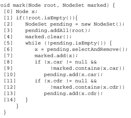
4.3.3 The Mark Procedure
Themarkprocedure shown in Fig. 5 implements the mark phase of a Mark&Sweep garbage collector.5
The procedure operates on a general graph, pointed by root. Therefore, the pre-condition is simplytrue. There is an f -edge from v1 tov2 if eitherv2 = v1.car or
v2 = v1.cdr. Note that unlike the previous examples, f is not deterministic. As an
optimization, we do not create copies off and root for each label of themark pro-cedure, because the procedure does not modifyf and root. We use unary relations p and m to denote objects in the pending and marked sets of nodes, respectively.
The postcondition formarkstates that a node is marked if and only if it is reachable fromroot: postmark
def
= postifmark∧post only−if
mark . The “if” part can be easily expressed
using the positive monadic formulam14(v
0) in the pattern, allowed in L1:
postifmark def
= root[f
→∗](¬null ⇒ m14)
5 This version is simplified because it assumes a single root object; a set of roots can be handled as shown in Section 9.
void mark(Node root, NodeSet marked) {
[0] Node x;
[1] if(!root.isEmpty()){
[2] NodeSet pending = new NodeSet(); [3] pending.addAll(root);
[4] marked.clear();
[5] while (!pending.isEmpty()) {
[6] x = pending.selectAndRemove(); [7] marked.add(x);
[8] if (x.car != null &&
[9] !marked.contains(x.car)) [10] pending.add(x.car); [11] if (x.cdr != null && [12] !marked.contains(x.cdr)) [13] pending.add(x.cdr); [14] } } }
Fig. 5. Themarkphase of a Mark&Sweep garbage collector.
The “only if” part requires reasoning about nodes that are not necessarily reachable fromroot. Moreover, it requires reasoning about nodes that need not be reachable from any program variable. To address it, we introduce a new constant cm which
represents an arbitrary node, because it is not restricted in the precondition, and write the postcondition and the loop invariant in terms of cm. Intuitively, when
checking validity of these formulas, the constantcm can be treated as a universally
quantified variable. In the postcondition, we require that ifcm is marked, then it is
reachable fromroot:
postonly−ifmark def
= m14(cm) ⇒ rooth→f ∗
icm
The loop invariant for mark consists of two parts. First, before the loop at label
[5] is entered for the first time, the only pending node is root, and no nodes are marked. In particular,root and cm are not marked. Second, after the loop was
executed at least some number of times, (i)root remains either marked or pending, (ii) a node cannot be both marked and pending, and (ii) most importantly, if a node is marked then its f -successor is either marked or pending. It means that the “frontier” of the exploration consists of pending nodes: there is no edge from a mark node to a node that is neither marked nor pending. Finally, if a node is marked or pending, then it is reachable fromroot, which implies the postcondition,
because the loop terminates when there are no pending nodes.
p5(root) ∧ (cm 6= root ⇒ ¬p5(cm)) ∧ (root[→f ∗ ]¬m5) ∧ ¬m5(c m) W (m5(root) ∨ p5(root)) ∧ root[f →∗](¬p5∨ ¬m5) ∧ (¬m5(c m) ∨ ¬p5(cm)) ∧ let t(v) def = f (v, v′) ∧ m5(v) ⇒ (m5(v′) ∨ p5(v′)) in root[f →∗]t ∧ m5(c m) ⇒ cm[→](pf 5∨ m5) ∧ p5(cm) ∨ m5(cm) ⇒ roothf →∗icm 4.4 TheL2 Fragment
The fragmentL2 extendsL1 by allowing constants to be freely used in patterns,
removing the last restriction of Def. 4.1. For example, the property that a general graph is a tree in which each node has a pointer b back to the root is expressible inL2, using the pattern true ⇒ b(v0, root), but this pattern is not in L1. It can be
shown that the property cannot be expressed inL1, using the same arguments as in
Section 7.
5 Decidability ofL1
In this section, we show thatL1is decidable for validity and satisfiability. SinceL1
is closed under negation, it is sufficient to show that it is decidable for satisfiability. The proof proceeds as follows:
(1) Translate anL0 formula into an equivalent MSO formula (Lemma 5.2).
(2) Define a class of simple graphsAk, for which the Gaifman graph (Def. 5.4) is
a tree with at mostk additional edges (Def. 5.5).
(3) Show that the satisfiability of MSO logic over Ak is decidable, by reduction
to MSO on trees [41] (Lemma 5.6). We could have also shown decidability using the fact that the tree width of all graphs inAkis bounded byk, and that
MSO over graphs with bounded tree width is decidable [15,2,48].
(4) Every formula ϕ ∈ L1 can be effectively translated into an equi-satisfiable
normal-form formula that is a disjunction of formulas in CL1 (Def. 5.9 and
Theorem 5.12). It is sufficient to show that the satisfiability of CL1 is
(5) Show that if formula ϕ ∈ CL1 has a model,ϕ has a model in Ak, where k
is proportional to the size of the formula ϕ (Theorem 5.14). This is the main part of the proof, given in detail in Section 6.
In Section 7, we extend this proof to show decidability ofL2.
5.1 Translation fromL0 to MSO
Every regular expression R can be effectively translated into an MSO formula ϕR(x, y), that describes the paths from x to y labeled with w, for every word w
inR. To encode the Kleene star expression, we use a least fixpoint operation, ex-pressible in MSO.
Lemma 5.1 Every routing expression R can be translated into an MSO formula
tr(R)(v1, v2) with two (first-order) free variables v1 and v2 such that for every
graphS and nodes a, b ∈ S, there is an R-path from a to b if and only if S, a, b |= tr(R)(v1, v2).
Sketch of Proof: For atomic regular expressions and concatenation, we definetr(R)(v1, v2)
as follows: tr(R)(v1, v2) def = f (v1, v2) ifR is→f f (v2, v1) ifR is←f ¬(c = v1) ∧ (v1 = v2) if R is ¬c u(v1) ∧ (v1 = v2) ifR is u ¬u(v1) ∧ (v1 = v2) ifR is ¬u tr(R1.R2)(v1, v2) def = ∃v3.tr(R1)(v1, v3) ∧ tr(R2)(v3, v2) The formula tr(R∗)(v
1, v2) holds when the minimal set Y that contains v1 and is
closed underR, contains v2. Formally, we define
tr(R∗)(v 1, v2)
def
= ∃Y.(v2 ∈ Y ) ∧ Q(v1, Y ) ∧ ∀Y′.Q(v1, Y′) ⇒ Y ⊆ Y′
whereQ(v1, Z) is (v1 ∈ Z) ∧ ∀v1′, v′2.(v1′ ∈ Z) ∧ ϕR(v1′, v′2) ⇒ (v2′ ∈ Z).
For example, the routing expression R def
= (n
→.¬y)∗ is translated into the MSO formulatr(R)(x, v) def
= ∃Y.(v ∈ Y ) ∧ Q(x, Y ) ∧ ∀Y′.Q(x, Y′) ⇒ Y ⊆ Y′, where
Q(x, Z) is (x ∈ Z) ∧ ∀v1′, v′2.(v1′ ∈ Z) ∧ ∃v3′.(f (v1′, v3′) ∧ ¬(x = v3′) ∧ (v′3 = v2′)) ⇒
(v′ 2 ∈ Z).
Using the translation of regular expressions as defined above, it is easy to translate a generalL0 formula to an equivalent MSO formula. Forϕ ∈ L0 overτ , T R2(ϕ)
is an MSO formula over the same vocabulary τ . The translation T R2 is defined
inductively: T R2(c[R]p) def = ∀v0, v1, . . . , vn.ϕR(c, v0) ⇒ p(v0, . . . , vn) T R2(ϕ1∧ ϕ2) def = T R2(ϕ1) ∧ T R2(ϕ2) T R2(¬ϕ1) def = ¬T R2(ϕ1)
For example, theL0 formulaϕ def
= xh n
→∗iy ∧ x[(→.¬y)n ∗]invn,n′ which is part of a
loop invariant of the reverse procedure (Section 4.3.1), is translated into the MSO formula
T R2(ϕ) = tr(→n∗)(x, y) ∧ ∀v0, v1.tr((→.¬y)n ∗)(x, v0) ⇒ (n(v0, v1) ⇒ n′(v1, v0))
wheretr(n
→∗) and tr((→.¬y)n ∗) are defined as above.
Lemma 5.2 For allϕ ∈ L0 and all graphsS, S |= ϕ iff S |= T R2(ϕ).
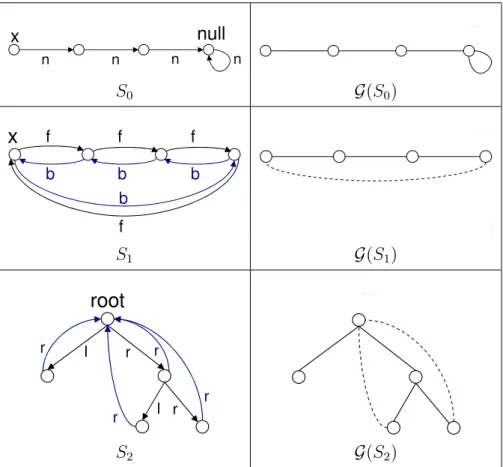
5.2 Decidability of MSO on Ayah Graphs
We define a notion ofTk, a set of undirected graphs each of which is a tree6 with
at mostk extra edges.
Definition 5.3 An undirected graphB is in Tk if removing self loops and at most
k additional edges from B results in an acyclic (undirected) graph.
For a directed graph we define the corresponding undirected graph:
Definition 5.4 Let G(S) denote the Gaifman graph of the graph S, i.e., an
undi-rected graph obtained fromS by removing node labels, edge labels, and edge di-rections (and parallel edges).
We define a notion of simple tree-like (directed) graphs, called Ayah graphs.
Definition 5.5 (Ayah Graphs) Fork ≥ 0, an Ayah graph of k is a graph S for
which the Gaifman graph is inTk:A
k= {S|G(S) ∈ Tk}.
Examples of graphs in A0, A1, and A2 are shown in Fig. 6. For j = 0, . . . , 2, a
structure Sj ∈ Aj is shown in the left column, and the corresponding Gaifman
6 In this paper, we use the term “tree” instead of the term “forest” to refer to an acyclic graph, possible undirected.
S0 G(S0)
S1 G(S1)
S2 G(S2)
Fig. 6. Examples of graphs inA0,A1, andA2. Forj = 0, . . . , 2, Sj ∈ Aj (left column) andG(Sj) ∈ Tj (right column). Dashed edges denote extra edges removing which results in a tree.
graphG(Sj) ∈ Tj is shown in the right column; withj dashed edges. Removing
the dashed edges fromG(Sj) yields a tree.
The graph S0 describes an acyclic singly-linked list pointed-to by x. The node
labeled with null does not represent an element of the list: it is a “sink” node which models thenullvalue, as explained in Section 4.2. InG(S0), the self-loop
is not dotted because Def. 5.3 ignores self-loops. (As we show later, self-loops can be easily handled, while larger cycles require a more complex treatment.) The graphS1 describes a cyclic doubly-linked list. In G(S1), a single edge represents
the parallel edges ofS1 with different directions and different labels. The graphS2
describes a tree with pointers from every tree node to the root. InG(S2), removing
a single edge cannot break both cycles, thus the graphS2 is inA2, but not inA1.
Remark. For every graphS in Ak, the tree width [44,16] ofG(S) is at most k + 1,
but can it can be strictly less than that. For example, a graph which consists of17 simple disjoint cycles is inA17, but its tree width is2.
The satisfiability problem of MSO logic on Ayah graphs can be reduced to the satisfiability problem of MSO logic on trees, which is decidable, using a classical result due to Rabin [41]. This reduction provides a constructive way to check
sat-isfiability ofL1 formulas, using an existing decision procedure for MSO on trees,
MONA [26].
The reduction consists of two satisfiability-preserving translations: The first is a translation T R3 from MSO on Ayah graphs to MSO on Σ-labeled trees, defined
below. The second is a translationT R4 from MSO onΣ-labeled trees to MSO on
(infinite) binary trees.
Lemma 5.6 There are translations T R3 and T R4 between MSO-formulas such
that for every MSO-formulaϕ, there exists a graph S ∈ Akthat satisfiesϕ if and
only if there exists a binary treeS′such thatS′ |= (T R
3◦ T R4)(ϕ).
In this paper, we describe only the translationT R3, and omit the (standard)
trans-lation,T R4.
5.2.1 EncodingAkGraphs asΣ-Labeled Trees
Given the vocabularyτ = hC, U, F i and a number k we define a new vocabulary τ′ = hC′, U′, {E}i, where E is the only binary relation, C′ = C ∪ {c1, . . . , ck} ∪
{d1, . . . , dk}, and U′ = {F f, Bf, Lf, Fd i f , Bd i f |f ∈ F, i = 1, . . . , k}).
LetΣ = P(C′∪ U′) be the set of all possible node labels from τ′. AΣ-labeled tree
is a graphS over τ′ that satisfies the following:
(1) TheE-edges form a directed forest: each node in S has at most one incoming E edge. An E-edge from node u1 to nodeu2 means thatu2 is a child ofu1 in
the tree.
(2) If a node has no incomingE-edge, then it must not be labeled by Ff, Bf, for
anyf ∈ F .
We useTΣto denote the set of allΣ-labeled trees.
Every graph inAk can be represented by aΣ-labeled tree. For example, consider
the cyclic doubly-linked listS1from Fig. 6, defined over the vocabularyτ with C =
{x}, U = {}, and F = {f, b}. The new vocabulary τ′ consists ofC = {x, c1, d1},
U = {Ff, Fb, Fd 1 f , Fd 1 b , Bd 1 f , Bd 1
b }, and F = {E}. The graph S1 can be represented
by the followingΣ-labeled tree (actually, it is a list in this example): Bd1 f , Fd 1 b Ff, Bb Ff, Bb Ff, Bb ÂÁÀ¿ »¼½¾ f //ÂÁÀ¿ »¼½¾ f //ÂÁÀ¿ »¼½¾ f //ÂÁÀ¿ »¼½¾ x, c1 d1
The graphS represented by a Σ-labeled tree has the same set of nodes as the tree. The labels ofS are defined as follows. A graph node is labeled with the constants and unary relation symbols that hold for the corresponding node in the tree. An
edge in the tree from node v to v′ represents edges between the corresponding
nodesv and v′in the graph. Additional labels on tree nodes represent the direction
and the labels of the graph edges adjacent to the corresponding nodes in the graph, as follows.
For each binary relation symbolf ∈ F , we introduce two unary relation symbols Ff andBf, denoting forward and backwardf -edge. If there is an edge from v to v′
in the tree, andv′ is labeled withF
f in the tree, then there is anf -edge from v to v′
inS. Similarly, if there is an edge from v′ tov in the tree, and v is labeled with B f
in the tree, then there is an f -edge from v to v′ in S. There is a self-loop of f on
a nodev in S if the node v in the tree is labeled with Lf. Also, each of thek pairs
of constantsci anddi in a tree represents edges between the nodes corresponding
toci anddi in the graph. Ifv is labeled with ci andFdi
f in the tree, then there is an
f -edge from v to the node labeled with di inS. If v is labeled with ci andBdi f in
the tree, then there is anf -edge from the node labeled with di tov in S.
For an MSO formulaϕ over τ , T R3(ϕ) is an MSO formula over the vocabulary τ′.
The translationT R3 is defined inductively onϕ, where the only interesting part is
the translation of a binary relation formulaf ∈ F :
T R3(f (v1, v2)) = (E(v1, v2) ∧ Ff(v2)) ∨(E(v2, v1) ∧ Bf(v1)) ∨(E(v1, v2) ∧ v1 = v2∧ Lf(v1)) Wk i=1 ((ci = v1∧ di = v2∧ Fd i f (v1)) ∨ (ci = v2∧ di = v1∧ Bd i f (v2)))
Lemma 5.7 Letϕ be an MSO formula. There is a graph S ∈ Ak such thatS |= ϕ
if and only if there is aΣ-labeled tree T ∈ TΣsuch thatT |= T R3(ϕ).
Proof: Given a graphS in Ak, we can encode it as a Σ-labeled tree T as follows.
First, remove all self loops and at mostk additional edges from the Gaifman graph ofS to obtain an acyclic undirected graph, U . It is easy to transform the undirected graphU into a directed forest T , by choosing one node in every connected compo-nent ofU as a root, and directing all edges from it downwards. Then, we can set the labels of T uniquely from the labels of the corresponding nodes in S. To encode that an edge inS is labeled with f , we identify the corresponding edge in T , and label the target of the edge with a unary relation to remember the labelf .
GivenT ∈ TΣ, we can uniquely reconstruct the graphS ∈ Ak that corresponds to
it. Every node inT that is labeled with Ff has exactly one incoming edge, which
defines the corresponding edge inS, labeled with f . For each Fdi
f , at most one edge
can be created inS, because T R3 guarantees that inT the source is labeled with ci,
and the target is labeled withdi, which are constants.
Proof: Follows from Lemma 5.6 and [41].
5.3 Normal Form ofL0Formulas
We define a normal-form formula to be a disjunction of conjunctions of formulas of the formchRic′andc[R]p.
Definition 5.9 (Normal-form formulas) A formula in CL0 is of the form ^ i ¬(ci[Ri]¬c′i) ∧ ^ j cj[Rj]pj
A normal-form formula is a disjunction of CL0formulas.
A formulaϕ is in CL1 if and only ifϕ ∈ CL0andϕ ∈ L1, i.e., all the patterns that
appear inϕ satisfy the requirement of Def. 4.1.
For a formulaϕ ∈ CL0, we useϕ✸to denote the first part ofϕ, namely V
i¬ci[Ri]¬c′i,
andϕ✷ to denote the second part ofϕ, namelyVjcj[Rj]pj. We use|ϕ✸| to denote
the number of conjuncts in the formulaϕ✸.
Note that while L0 is closed under negation, CL0 is not. The following theorem
shows that every L0-formula can be effectively translated into an equi-satisfiable
normal-form formula. The main difficulty is to translate a formula of the form ¬c[R]p, where p is an arbitrary pattern, into a formula in which negation appears only in front of constraints of the formc′[R]¬c′′.
Definition 5.10 Letθ be the formula ¬c[R]p over τ , where p(v0) = N (v0, . . . , vn) ⇒
ψ(v0, . . . , vn). We introduce new constant symbols c0, . . . , cn, and define τ′ =
τ ∪ {c0, . . . , cn}. We define tr(θ) as follows:
• Translate ¬ψ into an equivalent negated normal form formula ψ′,
• Let θ′ bechRic
0∧ N (c0, . . . , cn) ∧ ψ′(c0, . . . , cn)), where every edge formula
vi→vf j that appears inN or ψ′is replaced bycih→icf j. 7
• If ¬chRic′ appears inθ′, replace it withc[R]¬c′, to obtainθ′′.
• Transform θ′′into an equivalent disjunctive normal form formulaθ′′′.
• Let tr(θ) be θ′′′.
The formulatr(θ) is a normal-form formula by Def. 5.9, because it is a disjunction of CL0-formulas. In fact,tr(θ) is a very simple formula: all the patterns in it are of
the form true ⇒ c 6= v0. Thus, negation can appear only in front of reachability
constraints of the formc[R]¬c′whereR is star-free.
Lemma 5.11 For a graphS over τ , if S satisfies θ, then there exists an expansion of S to τ′, that satisfiestr(θ). For a graph S′overτ′, ifS′ |= tr(θ) then the restriction
S of S′ toτ satisfies ϕ.
Theorem 5.12 There is a computable translationT R1fromL0 to a disjunction of
formulas in CL0that preserves satisfiability.
Sketch of Proof: For every formulaϕ ∈ L0 over τ , the formula T R1(ϕ) is a
dis-junction of formulas in CL0overτ′ such thatϕ is satisfiable if and only if T R1(ϕ)
is satisfiable. The vocabulary τ′ is an extension ofτ with new constant symbols.
The translationT R1(ϕ) is defined as follows:
(1) Translate ϕ into an equivalent formula ϕ′ in negated normal form using
de-Morgan rules to push negations inwards.
(2) Replace every sub-formula¬c[R]p that appears in ϕ′ withtr(¬c[R]p), as in
Def. 5.10. The resulting formulaϕ′′is satisfiable if and only ifϕ′is satisfiable,
by Lemma 5.11. Note that this translation only preserves satisfiability (not equivalence).
(3) Translateϕ′′into an equivalent disjunctive normal form formulaϕ′′′. All atomic
formulas are of the formc[R]¬c′.
The result ofT R1(ϕ) is ϕ′′′.
The translation is applicable to the full L0 logic, in which case the reachability
constraints inϕ✷can contain arbitrary patterns.
The translation T R1 may introduce only patterns of the form true ⇒ c2 6= v0
beyond those patterns that appear in the input formula. This observation yields the following corollary:
Corollary 5.13 Forϕ ∈ L1, the translationT R1 returns a disjunction of formulas
in CL1(and preserves satisfiability).
5.4 Decidability ofL1
The following theorem states that CL1 has an Ayah-model property, i.e., every
satisfiable CL1formulaϕ has a model in Akwherek is defined by
f (ϕ) def
= 2 × n × |C| × |ϕ✸| (4)
Here, we assume that for every routing expression that appears in ϕ✸ there is an
equivalent automaton with at mostn states.
Theorem 5.14 (Ayah model property ofL1) If ϕ ∈ CL1 is satisfiable, thenϕ is
A non-trivial proof of this theorem is presented in Section 6.
Theorem 5.15 The satisfiability problem ofL1is decidable.
Proof: Follows from combining the results of Theorem 5.12, Theorem 5.14, Lemma 5.2, Theorem 5.8.
6 Ayah Model Property ofL1
In this section we provide a detailed proof of the main technical theorem of the paper, Theorem 5.14. Before diving into the details, we explain the main proof at a high-level.
Given a normal-form formulaϕ ∈ CL1 and a graphS such that S |= ϕ, we
con-struct a graphS′ and show thatS′ |= ϕ and S′ ∈ A k.
The construction operates as follows. We construct a pre-model S0 of S and ϕ,
which satisfies all constraints of the formchRic′ inϕ. The idea is to extract from S
a witness path for each constraint of the formchRic′ inϕ, and define S
0 to be the
union of these witness paths (Section 6.5).
The pre-model S0 may violate some of the constraints of the form c[R]p in ϕ.
Consider the case when the pattern p contains a positive occurrence of edge for-mula or equality forfor-mula. If a graph G violates a constraint c[R]p, then there is an enabled merge operation or edge-addition operation, depending on the patternp (Section 6.3).
For example, ifp is of the form N (v0, v1, v2) ⇒ v1 = v2, it defines a merge
op-eration. We say that this merge operation is enabled in a graphG (by c[R]p) when G contains a node w0 reachable by anR-path from c and distinct nodes w1 andw2
forming the neighborhood N (w0, w1, w2). Applying this operation means
merg-ing the nodes w1 andw2. After merging w1 andw2, other merge operations may
still be enabled in G by c[R]p. If there are no more enabled operations in G, then G |= c[R]p. Similarly, if p is of the form N (v0, v1, v2) ⇒ v1→vf 2, it defines an
edge-addition operation. Applying this operation means adding anf -edge.
Given a pre-model S0, we apply all enabled operations in any order, producing a
sequence of distinct graphsS0, S1, . . . until the last graph S′ has no enabled
opera-tions. Thus,S′ satisfies all constraints of the formc[R]p where p contains a positive
occurrence of edge formula or equality formula. We show that applying any enabled operation preserves witness paths for the constraints of the formchRic′. Thus, S′
also satisfies all constraints of the form chRic′. This construction also guarantees
thatS′ satisfies all the constraints of the formc[R]p where p is a negative formula. To show this formally, we use homomorphism (Section 6.4) which preserves
ex-istence of edges and both exex-istence and absence of labels on nodes (preserving absence of labels is non-standard).
Finally, the fact that S′ is in Ak is proved by induction. By construction, S0 is
in Ak (Lemma 6.11), and Ak is closed under operations enabled by L1 formulas
(Lemma 6.5). The proof of closure properties ofAkis based on closure properties
for a class of undirected graphs,Tk(Lemma 6.1).
The rest of the section describes the building blocks of the proof of Theorem 5.14: closure properties of Tk (Section 6.1), closure properties ofA
k (Section 6.2), the
definition of operations enabled byL1 formulas (Section 6.3), the definition of
ho-momorphism relation and its properties (Section 6.4), and the definition of witness splitting and properties of a pre-model (Section 6.5). The proof of Theorem 5.14 concludes the section.
6.1 Trees with Extra Edges
Recall from Def. 5.3 that Tk is a set of undirected graphs that are trees with k
extra edges. In this section we prove thatTk is closed under merging of vertices at
distance at most2.
The distance between the verticesv1andv2 in an undirected graphB is the number
of edges on the shortest path betweenv1andv2 inB.
Merging two vertices in an undirected graph is defined in the usual way, by gluing these vertices. Formally, let the undirected graphB′ denote the result of merging
nodesv1 andv2 inB. The set of vertices of B′ isVB ′ def
= (VB \ {v
1, v2}) ∪ {v12},
wherev12is a new vertex. Letm : VB → VB ′ be defined as follows: m(v) = v12 ifv = v1 orv = v2 v otherwise
If there is an edgee between the vertices v1 andv2 inB then there is an edge m(e)
betweenm(v1) and m(v2) in B. If there is an edge e between v1′ andv2′ inB′ then
there exist verticesv1 andv2 inB such that m(v1) = v1′,m(v2) = v′2, and there is
an edge betweenv1 andv2inB.
Lemma 6.1 Assume thatB is in Tkand verticesv
1 andv2 are at distance at most
two inB. The graph B′obtained fromB by merging v
1 andv2inB is also in Tk.
Proof: By definition of Tk, there exists a set of edges D ⊆ E such that B \ D,
denoted byT , is acyclic and |D| ≤ k. We show how to transform D into D′ ⊆ E′